warwick.ac.uk/lib-publications
Original citation:
Gagatsos, Christos N., Branford, Dominic and Datta, Animesh. (2016) Gaussian systems for
quantum-enhanced multiple phase estimation. Physical Review A, 94 (4). 042342.
Permanent WRAP URL:
http://wrap.warwick.ac.uk/83269
Copyright and reuse:
The Warwick Research Archive Portal (WRAP) makes this work by researchers of the
University of Warwick available open access under the following conditions. Copyright ©
and all moral rights to the version of the paper presented here belong to the individual
author(s) and/or other copyright owners. To the extent reasonable and practicable the
material made available in WRAP has been checked for eligibility before being made
available.
Copies of full items can be used for personal research or study, educational, or not-for-profit
purposes without prior permission or charge. Provided that the authors, title and full
bibliographic details are credited, a hyperlink and/or URL is given for the original metadata
page and the content is not changed in any way.
Publisher statement:
© 2016 American Physical Society
A note on versions:
The version presented here may differ from the published version or, version of record, if
you wish to cite this item you are advised to consult the publisher’s version. Please see the
‘permanent WRAP URL’ above for details on accessing the published version and note that
access may require a subscription.
PHYSICAL REVIEW A94, 042342 (2016)
Gaussian systems for quantum-enhanced multiple phase estimation
Christos N. Gagatsos, Dominic Branford, and Animesh Datta Department of Physics, University of Warwick, Coventry CV4 7AL, United Kingdom
(Received 20 May 2016; published 28 October 2016)
For a fixed average energy, the simultaneous estimation of multiple phases can provide a better total precision than estimating them individually. We show this for a multimode interferometer with a phase in each mode, using Gaussian inputs and passive elements, by calculating the covariance matrix. The quantum Cram´er-Rao bound provides a lower bound to the covariance matrix via the quantum Fisher information matrix, whose elements we derive to be the covariances of the photon numbers across the modes. We prove that this bound can be saturated. In spite of the Gaussian nature of the problem, the calculation of non-Gaussian integrals is required, which we accomplish analytically. We find our simultaneous strategy to yield no more than a factor-of-2 improvement in total precision, possibly because of a fundamental performance limitation of Gaussian states. Our work shows that no modal entanglement is necessary for simultaneous quantum-enhanced estimation of multiple phases.
DOI:10.1103/PhysRevA.94.042342
I. INTRODUCTION
Parameter estimation with quantum-enhanced precision has the potential to provide substantial technological advances as well as deep insights into the fundamental workings of Nature. Originating in the quest for the increased sensitivity requirements for detecting gravitational waves using laser interferometers with squeezed light [1,2], the field now en-compasses a variety of scenarios studying the quantum limits of sensing [3–6]. Relative phase estimation in a two-mode interferometer is by far the most common, although some attention has also been cast to the simultaneous estimation of multiple parameters at the quantum limit [7–13].
A fundamental bound on the precision of an estimation is the quantum limit on the variance of the estimator. This is set by the quantum Cram´er-Rao bound (QCRB) [14] and valuable insights into the working of quantum mechanics have been obtained by studying it in the multiparameter scenario [15–17]. In addition to this fundamental understanding, several scenarios of practical and technological interest are intrin-sically multiparameter estimation problems, leading to new methodologies of obtaining quantum enhancements arising purely from the multidimensional nature of the problem. This includes magnetic-field sensing in three dimensions [18] and imaging [10,19–21]. These proposed schemes use a fixed number of photons in multimode entangled states, which are not easy to prepare for increasing photon numbers.
Concerning Gaussian states and their role in estimation theory, general expressions have been derived which are useful for evaluating the quantum Fisher information matrix [22–27] but the explicit expressions found in these works are limited to two-parameter estimation problems. Reference [28] utilizes the quantum Ziv-Zakai bound [29] to numerically study the precision limit of up to 16-mode squeezed vacuum states and find in their example an improvement with simultaneous strategies without quantifying the factor of the improvement.
In this work we show that for an arbitrary number of phases and a fixedaverageamount of energy, simultaneous estimation (Fig. 1) of a fixed number of phase parameters is better than individual estimation (Fig. 2). We do so by obtaining an analytical expression for the quantum Fisher information
matrix (QFIM) as a function of the number of phases and the total average energy. In spite of the improvement found in the simultaneous case, we observe that under assumptions of equal magnitude squeezing in each mode and a multimode interferometer which is an orthogonal transform presents at most a factor-of-2 improvement, pointing to potential limitations of Gaussian states in multiparameter quantum metrology.
The QFIM bounds the covariance matrix for multiple phase estimation, and our results are derived for pure Gaussian states in terms of the Husimi Q function. Gaussian states are easier to prepare in practice than fixed particle number states, and while couched in the language of optical systems, our work also applies to bosonic degrees of freedom of matter systems. We show that our bounds are attainable, and discuss the implications of the factor-of-2 improvement.
Our work may thus improve the performance of optical techniques in quantum imaging [30] and possibly gravitational wave astronomy [31], as well as optomechanical systems employed in fundamental studies [32,33]. Some of these have been studied experimentally in quantum optics, where noise reduction has been observed using correlated photon pairs [34] and multimode squeezed light [35]. More interesting is the con-stant amount of improvement possible, unlike the fixedpeak energy scenario [10] where the improvement scales linearly with the number of parameters. While the limited quantum information processing capabilities of Gaussian states have long been recognized in computation and communication [36–39], ours is a possible instance in quantum metrology. It is interesting to note that this facet of quantum metrology only appears at the multiple phase level, since Gaussian states are known to achieve the full potential of quantum-enhanced single phase estimation [40].
The paper is organized as follows. In Sec.IIwe define the phase shifting, the simultaneous and the individual estimation scenarios. In Sec.IIIwe discuss the Cram´er-Rao bound and its attainability. In Sec.IVwe calculate analytically, under the assumptions we do later on, the QFIM and the trace of its inverse and in Sec.Vwe proceed with the comparison of the simultaneous and individual scenarios. Finally, in Sec.VIwe wrap up and discuss our findings.
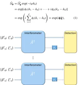
FIG. 1. Ad+1 mode interferometer with the most general pure Gaussian input, produced from a general pure and separable Gaussian state followed by a passive element. The resultant state undergoes the phase shifts to be estimated.
II. PHASE ESTIMATION SETUP
We study the quantum-limited estimation ofd phasesφ∈
Rd using a d+1-mode pure quantum probe state |, as shown in Fig.1. The state|picks up the phasesφvia| =
ˆ
Uφ|[41]. The parameters to be estimated are encapsulated in
ˆ
Uφ =Uˆφ exp(−iϕnˆ0)
=exp[iφ1( ˆn1−nˆ0)+ · · · +iφd( ˆnd−nˆ0)]
=exp
i
d
i=1
φi( ˆni−nˆ0)
=exp(iφgˆ), (1)
FIG. 2. A two-mode interferometer with the most general pure Gaussian input, produced from a general pure and separable Gaussian state followed by a passive element. The resultant state undergoes the phase shift to be estimated. This is repeated d times, i.e., for the number of phases to be estimated or it can be viewed as d
parallel, individual estimations. The total energy for simultaneous and individual estimation is the same.
where the unitary operator ˆUφ =exp(iφ0nˆ0+iφ1nˆ1+ · · · +
iφdnˆd),ϕ=φ0+ · · · +φd captures an unmeasurable overall phase,φ≡(φ1, . . . ,φd)T and ˆgi =nˆi−nˆ0are the generators. The ˆgi are traceless and Hermitian, as SU(n) generators ought to be. Indeed, our problem is a special case of SU(n) interferometry, with the parameters to be estimated restricted to a diagonal subgroup. The reduction of the phase-encoding unitary from an element of the unitary group to an element of the special unitary group is therefore tantamount to accounting for the unmeasurable (global) phaseφ. The nuanced role of a reference mode in quantum interferometry was recently addressed in Ref. [42].
The input| is taken to be a pure Gaussian state—the outcome of the interaction ofd+1 coherent squeezed states with a passive multimode quantum optical element ˆA† via | =Aˆ†dk=0|βk;ξk, where the squeezings ξk= |ξk|eiθk, and displacementsβkare introduced through the correspond-ing operators as ˆD(βk) ˆS(ξk)|0 = |βk;ξk. We are able to make the choice of complex displacements and positive squeezings without loss of generality [43] to still obtain a general pure Gaussian state [44].
Such a state has an average energy of|βk|2+sinh2|ξk|in modek,and our aim is to compare individual and simultaneous estimation strategies forφusing the same average input energy totalled over all the modes. The restriction to squeezed states is primarily motivated by the relative ease of production and manipulation in the laboratory, and demonstration of their relevance in studies of, for instance, quantum information science [45] and gravitational wave astronomy [46]. It also avoids, for a fixed mean, the possibility of unbounded variance in particle number. It is not to ease our analytical calculations, as we explain later.
III. BOUNDS ON PRECISION OF ESTIMATION
The performance of any estimation process is captured by the covariance matrixV(φ), the covariance of the estimators
for unbiased estimators. This is lower bounded as
V(φ)H−1, (2)
according to the quantum Cram´er-Rao bound, where H
is the quantum Fisher information matrix (QFIM) [3,47]. Equation (2) is a matrix inequality, meaningV(φ)−H−1 is positive semidefinite. The QFIMHis a real, positive definite, symmetric matrix. The QFIM can be written in terms of the symmetric logarithmic derivatives (SLDs); ˆLi for the phases
φi, are given by
∂ρˆφ
∂φi
= Lˆiρˆφ+ρˆφLˆi
2 . (3)
The QFIM is thenHi,j =Tr[ ˆρφ( ˆLiLˆj +LˆjLˆi)]/2.
[image:3.608.47.297.398.669.2]GAUSSIAN SYSTEMS FOR QUANTUM-ENHANCED . . . PHYSICAL REVIEW A94, 042342 (2016)
The attainability of the latter (quantum) equality is satisfied if the SLDs commute; this is sufficient to prove the existence of a saturating positive operator-valued measure (POVM), the common eigenbasis of the SLDs. In the case of single parameter estimation the existence of a saturating POVM is therefore trivial. A looser condition for the attainability of the latter (quantum) limit with pure states is [50,51]
|[ ˆLi,Lˆj]| =Tr( ˆρφ[ ˆLi,Lˆj])=0. (4) For commuting generators,
∂ρˆφ
∂φj
=i[ ˆgj,ρˆφ],
we find (with pure state probes) ˆLj =2i[ ˆgj,ρˆφ]. Using the fact that the generators commute, the cyclicity of the trace and purity of the probe states|, it is easy to show that the
condition in Eq. (4) is satisfied.
IV. COMPUTATION OF THE QFIM
For any pure state |, the QFIM reads Hi,j = 4Re(∂i|∂j − ∂i||∂j),where Re(·) denotes the real part and|∂i ≡(∂/∂φi)|. Fordphase parameters and the corresponding phase-shift generators{ˆgi}, thed×dQFIM reduces to [18]
Hi,j =4(gˆigˆj − gˆigˆj)
=4(hi,j−hi,0−h0,j+h0,0), (5) with hi,j = nˆinˆj − nˆinˆj. The expectation values are calculated for the initial state |. Note that for the matrix elements Hi,j the indices i,j run from 1 to d, while for the matrix elements hi,j the indices i,j run from 0 to d. Note that hi,0, h0,j, and h0,0 give rise to rank-1 matrices, and therefore the QFIM can be inverted using the Sherman-Morrison formula.
We use the Husimi Q representation to calculate the expectation values in Eq. (5). To that end, we begin with the
Qrepresentation [52] for the initial squeezed displaced states
d
k=0|βk;ξk,which reads
Q0(r)=
1
πd+1
d
k=0
|αk|βk;ξk|2
=F(β,β∗)exp(−r
†Mr+r†
br+r†rb) (2π)d+1d
k=0cosh|ξk|
, (6)
where|αkis a coherent state,
r=(α,α∗)T ≡(α0, . . . ,αd,α0∗, . . . ,α∗d) T,
(7)
rb=(b,b∗)T ≡(b0, . . . ,bd,b∗0, . . . ,b∗d)T, (8)
wherebj =dj=0(βk+βk∗tanh|ξk|),
F(β,β∗)=
d
k=0 exp
− |βk|2+
tanh|ξk| 2
βk∗2+βk2,
M= 1
2
I D
D I
,
and D is a diagonal matrix with Dj,j =tanh|ξj|. The Q representation of the final probe state | is then given byQ(α)= |α||2,whereα=Aα.Our calculation thus exploits the simplicity of applying ˆA on the coherent state basis rather than its conjugate on the squeezed displaced states. Further simplification is enabled by the passive nature of the transformation ˆA which implies|α|2= |α|2 and the φ independence of the QFIM, which can be seen in Eq. (5). The
Qrepresentation of|is thus (see Appendix Sec.1)
Q(r)=F(β,β∗)exp(−r
†Mr+r†
br+r†rb) (2π)d+1d
k=0cosh|ξk|
, (9)
with rb=(b,b∗)T ≡(b0, . . . ,bd,b∗0, . . . ,b∗d) T
, and bj = d
k=0A∗kj(βk+βk∗tanh|ξk|).The 2(d+1)×2(d+1) matrix
Mreads
M= 1
2
I N
N† I
,
withN=A†DA∗.Note that matrixNis symmetric, i.e.,N= NT, a fact to be exploited later.
To calculate the QFIM in Eq. (5) using theQrepresentation of the probe state | at hand, we need to recast the expectation values in terms of antinormally ordered operators. These are nˆi = aˆiaˆi† −1 and nˆinˆj =1+ aˆiaˆjaˆ†iaˆj† − aˆjaˆj† −(1+δij)aˆiaˆ†iand can be obtained via a generating functionG(μ) (see Appendix Sec.2),
nˆi = −1+
∂ ∂λi
∂ ∂λ∗i
G(μ)
μ=0
, (10)
nˆinˆj =1+
∂ ∂λi
∂ ∂λ∗i
∂ ∂λj
∂
∂λ∗j −
∂ ∂λj
∂ ∂λ∗j
−(1+δi,j)
∂ ∂λi
∂ ∂λ∗i
G(μ)
μ=0
. (11)
The generating function, which is based on theQ representa-tion in Eq. (9) is given by (see Appendix Sec.2),
G(μ)=exp
r†bM−1μ+μ†M−1rb+μ†M−1μ 4
, (12)
whereμ=(λ0, . . . ,λd,λ∗0, . . . ,λ∗d) T
. Note that the derivatives required to calculate the QFIM render the relevant integrals non-Gaussian. Finally, the inverse of M, obtained using Schur’s complement, is
M−1=2 E −NE
T −N†E ET
, (13)
where E=A†CAwithCa diagonal matrix whose nonzero elements readCj,j =cosh2|ξj|. Note thatE†=E.
By virtue of Eqs. (10)–(12), the elementshi,j are
hi,j =4[(EN−γ γT)◦(EN−γ γT)∗−(γ γT)◦(γ γT)∗
+1
4(E+E∗)◦(E+E∗+2γ γ†+2γ∗γ
T )
−(E+γ γ†)◦I]i,j, (14) where γ =(2E∗−E∗N∗−N∗E)b/2,δi,j is the Kronecker δ and◦denotes the Hadamard (entrywise) product.
Having obtained the general formula for the QFIM, we make two simplifying assumptions to obtain tractable analytical expressions, namely equally squeezed inputs in all the modes (|ξi| = |ξ|,∀i∈ {0, . . . ,d}) and an orthogonal interferometer (A†=OT ∈SO(d+1)). What follows in this work relies on these assumptions. For general displacements
βk=xk+iyk, a straightforward computation leads to a diagonal plus a rank-1 matrix,
Hi,j =δi,jhi,i+h0,0, (15)
where hi,i =2 sinh22|ξ| +4e−2|ξ|xi2+4e2| ξ|y2
i and h0,0= 2 sinh22|ξ| +4e−2|ξ|x2
0 +4e2|
ξ|y2
0 with xi= d
k=0O
T i,kxk andyi=dk=0Oi,kT xk. In matrix notation the QFIM reads
H=H+h0,0uuT, (16)
whereHi,j =δi,jhi,iandu=(1, . . . ,1)T.
We can now bound the total variance of all the parameters, given by Tr[V(φ)]. This requires the inverse of the QFIM which, obtained by the Sherman-Morrison formula, is
H−1=H−1− h0,0
1+h0,0uTH−1u
H−1uuTH−1, (17)
leading to
Tr(H−1)= d
i=1 1
hi,i −
d
i=0 1
hi,i −1 d
i=1 1
h2i,i. (18)
V. SIMULTANEOUSV SINDIVIDUAL PHASE ESTIMATION
The optimal input for estimating the relative phase in a balanced two-mode interferometer is a squeezed state [40]. We extend this result within the aforementioned assumptions and prove that for anyd,all the energy should go to squeezing for maximal precision in estimation. We do this by first showing that minimizing Tr(H−1) is akin to maximizing each hi,i independently. Note thathi,i is actually a monotonic function of the fraction of the total energy in displacements, and we show that this quantity is maximum when all the energy is used in squeezing (see Appendix Sec. 3). This leads to an optimal QFIM for simultaneous estimation of
Hsim=2(I+uuT) sinh22|ξ|. (19)
The QFIMHindfor individual phase estimation comes from the above equation withd=1.We can now compare the quantum limits for the simultaneous estimation of the d phases with their individual estimation for the same expense of energy. The total energy isE=di=0(x2
i +yi2)+(d+1) sinh
2|ξ| =
2dsinh2|ξ|, where ξ is the squeezing used for individual estimation. The ratio of the performance of the two estimation strategies is given by
R= Tr
H−sim1
TrH−ind1 =1−
d−1
2d tanh
2|ξ|. (20)
In Fig. 3 the behavior of R as a function of |ξ| and d is shown. Since R1, the simultaneous estimation strategy is superior to the individual estimation strategy. It is also easy to see thatR(1+1/d)/2.That the ratioR saturates
5
10
15
20
0.0
0.5
1.0
1.5
2.0
d
R
[image:5.608.325.544.68.246.2]0.65 0.75 0.85 0.95
FIG. 3. Ras a function of number of phases and squeezing.
to 1/2 is unlike the fixed photon number scenario [10] where the limit goes to 0, although in both cases they fall linearly withd. Possible causes for this are the restriction to Gaussian systems and our assumptions of equal squeezing and orthogonal transformations.
In the limit of a large number of phase parameters,
Rlim= lim
d→∞R=1−
1 2tanh
2|ξ|. (21)
Increasing squeezing is a matter of continuous improvement with state-of-the-art experimental setups, and in Fig. 4 we plot Rlim for up to 16 dB squeezing [53], i.e., |ξ| ≈1.84 (dB=10 log10e2|ξ|). Experimentally, squeezings of 12.7 dB have been achieved [54] along with multimode squeezings of 3.5 dB [35].
VI. CONCLUSIONS
[image:5.608.325.545.565.716.2]We have considered the problem of multiple phase es-timation with Gaussian states and have shown that, under some assumptions, the simultaneous estimation ofdphases is always superior to the optimum individual estimation strategy. A tentative cause for this improvement is that the simultaneous
GAUSSIAN SYSTEMS FOR QUANTUM-ENHANCED . . . PHYSICAL REVIEW A94, 042342 (2016)
strategy utilizes fewer reference modes, allowing more energy per mode. Our analyses have shown that the larger the variance within a mode the better the estimation. The optimal input states for individual and simultaneous strategies are product squeezed vacuum states and so the distinction boils down to the number of modes; as the simultaneous strategy uses fewer reference modes it allows a larger variance per mode and thus an improved precision. It may be for related reasons that the high-energy limit of the performance ratio of the two strategies coincides with the ratio of the number of modes, (d+1)/2d.
It can be noted that these quantum enhancements are obtained from simultaneous estimation without the presence of any quantum entanglement across the modes in the system. The latter is a consequence of the two assumptions: equal magnitude squeezings and an orthogonal transformation, which we made to obtain analytically tractable expressions. Nevertheless, this provides—as also claimed in Ref. [13]—a possible generalization of what was known for single phase
estimation [40,55,56] to multimode interferometry, that modal entanglement is not a crucial resource for quantum-enhanced interferometry.
Our analysis has shown that simultaneous multiple phase estimation is only a factor of 2 better than individual phase estimation using pure Gaussian states. This is true for any numberdof phases, while with non-Gaussian states the same scenario offers a factor-of-d improvement [10]. The limit of a factor-of-2 improvement in multimode Gaussian systems as opposed to a factor ofdwith non-Gaussian states seems unique to the multiparameter aspect of the problem.
ACKNOWLEDGMENTS
We thank T. Baumgratz and G. Knee for useful dis-cussions. This work was supported by the UK EPSRC (EP/K04057X/2) and the National Quantum Technologies Programme (EP/M01326X/1, EP/M013243/1).
APPENDIX
1. Computation of theQrepresentations
Initially we considerd+1 squeezed displaced states, i.e.,dk=0|βk;ξk, whereξk= |ξk|eiθk. From the definition of theQ representationQ(r)=1/πd+1α|ρˆ|α, withr=(α,α∗)T ≡(α
0, . . . ,αd,α∗0, . . . ,αd∗) T
, one can immediately write
Q0(r)= 1
πd+1
d
k=0
|αk|βk;ξk|2. (A1)
The amplitudeα|β;ξcan be found as follows:
α|β;ξ = √ 1
cosh|ξ|exp −
|β|2 2 −
β∗
2 e iθ
tanh|ξ|
∞
n=0 1 √
n!Hn(τ)
eiθtanh|ξ| 2
n/2 α|n
= √ 1
cosh|ξ|exp −
|β|2
2 −
β∗
2 e iθ
tanh|ξ| −|α|
2
2
∞
n=0 1
n!Hn(τ)
a∗2eiθtanh|ξ|
2
n/2
= √ 1
cosh|ξ|exp −
|α|2 2 −
|β|2 2 +βα
∗−1 2e
iθ
tanh|ξ|(α∗−β∗)2
, (A2)
whereHn(τ) is the Hermite polynomial of thenth order withτ =(β+β∗eiθtanh|ξ|)/(2eiθtanh|ξ|)1/2. We have also used the expansion of a squeezed state in Fock basis [57] and the Hermite polynomials generating function [58],
∞
n=0 1
n!Hn(τ)
u
2
n
=exp(2τ u−u2). (A3)
From Eqs. (A1) and (A2) we write
Q0(r)=
1
πd+1d
k=0cosh|ξk| d
k=0
exp
−|αk|2 2 −
|βk|2 2 +βkα
∗ k−
1 2e
iθktanh|ξ
k|(αk∗−βk∗)2
2
= 1
πd+1d
k=0cosh|ξk|
×exp
d
k=0
−|αk|2− |βk|2+βkα∗k+βk∗αk− 1
2tanh|ξk|[e iθk(α∗
k−βk∗)2+e− iθk(α
k−βk)2]
. (A4)
The statedk=0|βk;ξkgoes through the interferometer denoted as ˆA†and we take the state| =Aˆ† d
k=0|βk;ξk. TheQ representation of the|state is
Q(r)= 1
πd+1
α|Aˆ†
d
k=0 |βk;ξk
2
. (A5)
It is apparent that it is a lot easier if we act with ˆA†on the left, i.e., ona|, that is we consider the transformationα=Aαor
αk =dj=0Ak,jαj. Note that since we consider passive transformations the total energy before and after the interferometer is conserved, i.e.,dk=0|αk|2=
d
k=0|αk|2. Applying the transformation and working out Eq. (A5) a bit we get,
Q(r)= 1
πd+1d
k=0cosh|ξk| exp
− d
k=0
|βk|2+ 1
2tanh|ξk|
eiθkβ∗2
k +e− iθkβ2
k
×exp
⎡ ⎢ ⎣−
d
k=0
⎧ ⎪ ⎨ ⎪ ⎩|αk|
2+1
2tanh|ξk|
⎡ ⎢ ⎣eiθk
⎛ ⎝d
j=0
A∗k,jαj∗
⎞ ⎠
2
+e−iθk
⎛ ⎝d
j=0
Ak,jαj ⎞ ⎠
2⎤
⎥ ⎦ ⎫ ⎪ ⎬ ⎪ ⎭ ⎤ ⎥ ⎦
×exp
⎡ ⎣d
k=0
βk ⎛ ⎝d
j=0
A∗k,jα∗j +e−iθktanh|ξ
k| d
j=0
Ak,jαj ⎞ ⎠ ⎤ ⎦
×exp
⎡ ⎣d
k=0
βk∗
⎛ ⎝d
j=0
Ak,jαj +eiθktanh|ξk| d
j=0
A∗k,jα∗j
⎞ ⎠ ⎤
⎦. (A6)
By observing Eq. (A6) we can write it in a compact form,
Q(r)=F(β,β∗)exp(−r
†Mr+r†
br+r†rb) (2π)d+1d
k=0cosh|ξk|
,
where
F(β,β∗)=e−kd=0[|βk|2+(1/2) tanh|ξk|(eiθkβk∗2+e−iθkβk2)], (A7)
β=(β0, . . . ,βd), (A8)
β∗=(β∗
0, . . . ,βd∗), (A9)
rb =(b0, . . . ,bd,b∗0, . . . ,b∗d) T =
(b,b∗)T (A10)
with
bj =
d
k=0
A∗kj(βk+βk∗e
iθktanh|ξ
k|). (A11)
The 2(d+1)×2(d+1) matrixMreads
M= 1
2
I N
N† I
(A12)
withN=A†DA∗,whereDis a diagonal matrix withDj,j =eiθjtanh|ξj|.Note that matrixNis symmetric, i.e.,N=NT. Also the matrixMis Hermitian. In what follows we will need the matrixM−1; to this end we will use Schur’s complement [59]. We write
M−1=2
(I−NN†)−1 −N(I−N†N)−1 −N†(I−NN†)−1 (I−N†N)−1
GAUSSIAN SYSTEMS FOR QUANTUM-ENHANCED . . . PHYSICAL REVIEW A94, 042342 (2016)
From Eqs. (A12) and (A13) it is easy to see thatM−1M=I. For the Hermitian matricesNN†andN†Nwe can readily write their diagonalization (remember thatAis unitary, therefore they diagonalize Hermitian matrices),
NN†=A†DD†A, (A14)
N†N=ATDD†(AT)†. (A15)
SinceA†A=Iand (AT)†AT =Iwe have
(I−NN†)−1=A†(I−DD†)−1A, (A16)
(I−N†N)−1=AT(I−DD†)−1(AT)†. (A17)
The matrix (I−DD†)−1≡C. Since (I−DD†)−1is a diagonal matrix, the matrix Cis easily found to be the diagonal matrix whose nonzero elements readCj,j =cosh2|ξj|. Therefore from Eqs. (A13), (A16), and (A17) we write
M−1=2 E −NE
T −N†E ET
, (A18)
whereE=A†CA.
Let us now prove that the matrixMis not only Hermitian but also positive semidefinite and therefore can be used in the next section as a complex covariance matrix. We will calculate the (real) eigenvaluesσof the (Hermitian) matrixM. The characteristic polynomial reads
det(M−σI)=det
1
2 −σ
I 12N
1 2N†
1
2 −σ
I
=0. (A19)
Since the blocks in Eq. (A19) are square andN†commutes with (12−σ)I, from [60] we can write
det(M−σI)=det 1 2−σ
2
I−1
4NN
†
=0. (A20)
By virtue of Eq. (A14) and the facts thatAis unitary andM−σIis Hermitian, and by substituting the elements of the diagonal matricesDandD†, we can write
det(M−σI)=det 1 2−σ
2
I−1
4DD
†
= d
i=0 1 2 −σi
2 −1
4tanh 2|ξ
i|
=0. (A21)
From Eq. (A21) we readily find
σi =12(1∓tanh|ξi|)0. (A22)
2. Generating function and mean values
We introduce the generating functionG(μ),
G(μ)=
"
drQ(r) exp
⎛ ⎝d
j=0
λjα∗j + d
j=0
λ∗jαj ⎞
⎠, (A23)
whereμ=(λ0, . . . ,λd,λ∗0, . . . ,λ∗d) T
. Theλ’s are the so-called sources [61], nothing else than some helping parameters when it comes to calculating somewhat difficult integrals [62]. The wordsourcescomes from the fact that some linear terms are added into the exponential. Sometimes this is referred to asFeynman’s favorite trick. It is not difficult to see that the integral in Eq. (A23) is just a Gaussian integral and is therefore easy to be calculated. Also observe that when we hit Eq. (A23) with derivatives with respect toλ’s atμ=0, we get expectation values of combinations of ˆa,aˆ†, that justifies the namegenerating function. This is exactly what we need in order to calculate the QFIM for pure states. Since we use theQrepresentation formalism we must calculate expectation values in terms of the mean values of antinormally ordered operators, i.e., all creation operators should be
on the right,
nˆi = ˆaiaˆi† −1, (A24)
nˆinˆj = aˆiaˆjaˆi†aˆ
†
j − aˆiaˆi† − aˆjaˆ†j − aˆiaˆ†iδij+1,
(A25)
where we have used [ ˆa,aˆ†]=1. From Eqs. (A23)–(A25) it is not difficult to see that
nˆi =
∂ ∂λi
∂ ∂λ∗i
G(μ)
μ=0
−1, (A26)
nˆinˆj =
∂ ∂λi
∂ ∂λ∗i
∂ ∂λj
∂
∂λ∗j −(1+δij) ∂ ∂λi
∂ ∂λ∗i −
∂ ∂λj
∂ ∂λ∗j
G(μ)
μ=0
+1. (A27)
So, we have transformed the problem of calculating a non-Gaussian integral (when calculating the mean photon number for example) into one of calculating a Gaussian integral and its derivatives up to fourth order.
In Eq. (A23) bydrwe denote integration over all Reαand Imα. However, we find it more convenient to calculate the integral overαandα∗. To this end we will need the Jacobian for the transformation (Reα,Imα)→(α,α∗), which reads 1/2d+1. By doing the Gaussian integral of Eq. (A23) we find the generating function,
G(μ)=F(β,β∗)exp[(r
†
b+μ†)M−1(rb+μ)] 2d+1detMd
k=0cosh|ξk|
, (A28)
whereF(β,β∗) was defined in Eq. (A7).
We can simplify the generating function even more by noting thatG(μ=0)=1 since this is simply the integration of theQ
representation over all phase space, i.e., this is just the normalization to 1 of theQquasiprobability distribution. Therefore we get
G(μ)=exp#14(r†bM−1μ+μ†M−1rb+μ†M−1μ) $
. (A29)
Now the job is straightforward, easy, and boring; by carefully performing the derivatives of Eqs. (A26) and (A27) one finds the matrix elementshi,j and therefore the QFIM found in the main body of the text.
3. Optimization
We have given the expression for Tr(H−1) in terms of the elementshi,iunder the assumptions that we have an equal squeezing in each mode and that the unitary transform is an orthogonal transform as
Tr(H−1)= d
i=1 1
hi,i −
d
i=0 1
hi,i −1 d
i=1 1
h2
i,i
. (A30)
We can rewritehi,i =2 sinh22|ξ| +4e−2|ξ|xi2+4e2|ξ|yi2in terms of someEj =sinh2|ξ| +xj2+yj2, andEγj =x
2
j +yj2and
θγj =cos−
1(√xj
Eγj). Under this parametrization the energy constraint becomes d
j=0Ej =ETot [63]. We thus write hj,j =
hj,j(Ej,Eγj,θγj) and can now extremize Tr(H−
1) overE
γj andθγj without needing to construct a Lagrangian problem (as the
only constraint onEγj andθγj is 0Eγj Ej). We now consider what we need to solve in order to extremize Tr(H−
1) with
respect tomj =Eγj,θγj forj =0 [64],
∂Tr(H−1)
∂mj
= ∂hj,j
∂mj
⎡ ⎣− 1
h2 j,j + 2 h3 j,j d
i=0 1 hi,i −1 − 1 h2 j,j d
i=0 1
hi,i −2 d
i=1 1
h2
i,i ⎤ ⎦
= −∂hj,j
∂mj 1 h2 j,j d
i=0 1
hi,i −2⎡
⎣ d
i=0 1 hi,i 2 − 2 hj,j d
i=0 1
hi,i +
d
i=1 1
h2
i,i ⎤
⎦. (A31)
We first note that the terms in the square brackets can be rewritten (forj =0) as
⎛ ⎝ d
i=0,i=j 1 hi,i ⎞ ⎠ 2 + 2 hj,j d
i=0 1 hi,i − 2 hj,j d
i=0 1
hi,i +
d
i=1,i=j 1
h2
i,i
GAUSSIAN SYSTEMS FOR QUANTUM-ENHANCED . . . PHYSICAL REVIEW A94, 042342 (2016)
The middle two terms cancel and the remaining terms are clearly positive. Thus we may freely conclude that
∂Tr(H−1)
∂mj
= −κ∂hj,j
∂mj
, κ >0. (A33)
Namely, to extremizehj,j with respect tomj is to extremize Tr(H−1) with respect tomj; furthermore asκ >0 if a change in
mj increaseshj,j then it necessarily decreases Tr(H−1). We now therefore turn our attention to the maximization ofhj,j with respect toEγj andθγj,
hj,j =4
#
−Eγj +2Ej
1+Ej−Eγj
$
+8Eγj
%
Ej −Eγj
1+Ej −Eγj
cos 2θγj. (A34)
=10 No further mathematics is required to see thathj,jis maximized with respect toθγjbyθγj =0, which reduces the problem
to
hj,j =4
#
−Eγj +2Ej
1+Ej −Eγj
$
+8Eγj
%
Ej −Eγj
1+Ej −Eγj
, (A35)
∂hj,j
∂Eγj
=−4−8Ej+8 %
Ej −Eγj
1+Ej−Eγj
+4Eγj
−1−2Ej +2Eγj
%
Ej −Eγj
1+Ej −Eγj
=0. (A36)
We can then solve Eq. (A36) to find the solutions &(Ej −Eγj)(1+Ej −Eγj)= −Eγj and
&
(Ej −Eγj)(1+Ej −Eγj)=
Ej+Eγj +
1
2. Both of these entailEγj to lie outside of 0Eγj Ej (the former obviously so, the latter solutions requires
the similarly unacceptableEγj = −
1
8(1+2Ej)). To this end there are no extrema within the allowed values ofEγj insteadhj,j is
monotonic within those values. To this end we consider the extreme cases,Eγj =0 andEγj =Ej, which yield respectively hj,j =8Ej(Ej +1) andhj,j =4Ej.Eγj =0 could have been expected to yield the superior solution asEγj =Ejcorresponds to
the use of a coherent state. We are now left to optimize Tr(H−1) over{E
j}subject to d
j=0Ej =ETot, however asEγj =sinh
2|ξ
j| we have previously assumed|ξj| = |ξ|,∀j ∈ {0, . . . ,d}which takes us toEj = Ed+Tot1; this leads us to the optimal QFIM,
Hsim=2(I+uuT) sinh22|ξ|
=8(I+uuT)ETot(d+1+ETot)
(d+1)2 . (A37)
[1] C. M. Caves,Phys. Rev. D23,1693(1981). [2] R. X. Adhikari,Rev. Mod. Phys.86,121(2014). [3] M. G. A. Paris,Int. J. Quantum Inf.07,125(2009).
[4] V. Giovannetti, S. Lloyd, and L. Maccone,Nat. Photon5,222
(2011).
[5] R. Demkowicz-Dobrza´nski, M. Jarzyna, and J. Kołody´nski, Progress in Optics (Elsevier, Amsterdam, The Netherlands, 2015), Vol. 60, pp. 345–435.
[6] G. T´oth and I. Apellaniz,J. Phys. A47,424006(2014). [7] H. P. Yuen and M. Lax,IEEE Trans. Inf. Theory19,740(1973). [8] A. Fujiwara, Math. Eng. Tech. Rep 94-9 (1994),
http://www.keisu.t.u-tokyo.ac.jp/research/techrep/data/1994/ METR94-09.pdf.
[9] M. G. Genoni, M. G. A. Paris, G. Adesso, H. Nha, P. L. Knight, and M. S. Kim,Phys. Rev. A87,012107(2013).
[10] P. C. Humphreys, M. Barbieri, A. Datta, and I. A. Walmsley,
Phys. Rev. Lett.111,070403(2013).
[11] P. J. D. Crowley, A. Datta, M. Barbieri, and I. A. Walmsley,
Phys. Rev. A89,023845(2014).
[12] Y. Yao, L. Ge, X. Xiao, X. Wang, and C. P. Sun,Phys. Rev. A 90,062113(2014).
[13] P. Knott, T. Proctor, A. Hayes, J. Ralph, P. Kok, and J. Dunningham,arXiv:1601.05912.
[14] S. L. Braunstein and C. M. Caves,Phys. Rev. Lett.72,3439
(1994).
[15] R. D. Gill and S. Massar,Phys. Rev. A61,042312(2000). [16] M. D. Vidrighin, G. Donati, M. G. Genoni, X.-M. Jin, W.
S. Kolthammer, M. S. Kim, A. Datta, M. Barbieri, and I. A. Walmsley,Nat. Commun.5,3532(2014).
[17] D. W. Berry, M. Tsang, M. J. W. Hall, and H. M. Wiseman,
Phys. Rev. X5,031018(2015).
[18] T. Baumgratz and A. Datta,Phys. Rev. Lett.116,030801(2016). [19] Y. Yao, L. Ge, X. Xiao, X.-g. Wang, and C.-p. Sun,Phys. Rev.
A90,022327(2014).
[20] J.-D. Yue, Y.-R. Zhang, and H. Fan,Sci. Rep.4,5933(2014). [21] L. Liberman, Y. Israel, E. Poem, and Y. Silberberg,Optica3,
193(2016).
[22] A. Monras and F. Illuminati,Phys. Rev. A81,062326(2010). [23] A. Monras and F. Illuminati,Phys. Rev. A83,012315(2011). [24] A. Monras,arXiv:1303.3682.
[25] Y. Gao and H. Lee,Europhys. J. D68,1(2014).
[26] D. ˇSafr´anek, A. R. Lee, and I. Fuentes,New J. Phys.17,073016
(2015).
[27] L. Banchi, S. L. Braunstein, and S. Pirandola,Phys. Rev. Lett. 115,260501(2015).
[28] Y.-R. Zhang and H. Fan,Phys. Rev. A90,043818(2014).
[29] M. Tsang,Phys. Rev. Lett.108,230401(2012).
[30] M. I. Kolobov and C. Fabre,Phys. Rev. Lett.85,3789(2000). [31] Gravitational Wave International Committee, “The GWIC
roadmap. The future of gravitational wave astronomy”, 2010,
https://gwic.ligo.org/roadmap/.
[32] A. Arvanitaki and A. A. Geraci,Phys. Rev. Lett.110,071105
(2013).
[33] A. D. K. Plato, C. N. Hughes, and M. S. Kim,Contemp. Phys. 57,477(2016).
[34] G. Brida, M. Genovese, and I. Ruo Berchera,Nat. Photon.4,
227(2010).
[35] C. S. Embrey, M. T. Turnbull, P. G. Petrov, and V. Boyer,Phys. Rev. X5,031004(2015).
[36] S. D. Bartlett, B. C. Sanders, S. L. Braunstein, and K. Nemoto,
Phys. Rev. Lett.88,097904(2002).
[37] J. Eisert, S. Scheel, and M. B. Plenio,Phys. Rev. Lett.89,137903
(2002).
[38] J. Fiur´aˇsek,Phys. Rev. Lett.89,137904(2002).
[39] G. Giedke and J. I. Cirac,Phys. Rev. A66,032316(2002). [40] M. D. Lang and C. M. Caves,Phys. Rev. A90,025802(2014). [41] In what follows, calligraphic and/or hatted alphabets such as
ˆ
A,Uˆ,nˆ denote operators, while bold upper-case alphabetsA,U
denote their matrix representations (or other matrices, depending on the context). Letters with two indices such asAi,j,Ui,j,hi,j represent matrix elements. Bold lower-case characters denote vectors such asφ.
[42] M. Jarzyna and R. Demkowicz-Dobrza´nski,Phys. Rev. A85,
011801(2012).
[43] A local rotation ˆUk(ωk) acting on a squeezed state|γk,|ξk|eiθk gives ˆUk(ωk)|γk,|ξk|eiθk = |γke−iωk,|ξk|ei(θk−ωk/2). By choos-ingωk=2θkwe get|βk,|ξk|, whereβk=γke−2iθk (note thatβk andγkare left to be arbitrary complex numbers). The conjugate transpose of the local rotations ˆUk(2θk) can be considered as part of the the general transformation ˆA†which will now act on the squeezed states|βk,|ξk|to still give a general pure Gaussian state.
[44] S. L. Braunstein,Phys. Rev. A71,055801(2005).
[45] N. J. Cerf, G. Leuchs, and E. S. Polzik,Quantum Information With Continuous Variables of Atoms and Light(Imperial College Press, London, UK, 2007).
[46] R. Schnabel, N. Mavalvala, D. E. McClelland, and P. K. Lam,
Nat. Commun.1,121(2010).
[47] C. Helstrom,Quantum Detection and Estimation Theory (Aca-demic, New York, 1976).,
[48] S. L. Braunstein,J. Phys. A25,3813(1992).
[49] R. Blandino, M. G. Genoni, J. Etesse, M. Barbieri, M. G. A. Paris, P. Grangier, and R. Tualle-Brouri,Phys. Rev. Lett.109,
180402(2012).
[50] K. Matsumoto,J. Phys. A35,3111(2002).
[51] M. Szczykulska, T. Baumgratz, and A. Datta, Advances in Physics: X,1(2016).
[52] M. Hillery, R. O’Connell, M. Scully, and E. Wigner,Phys. Rep. 106,121(1984).
[53] R. Demkowicz-Dobrza´nski, K. Banaszek, and R. Schnabel,
Phys. Rev. A88,041802(2013).
[54] T. Eberle, S. Steinlechner, J. Bauchrowitz, V. H¨andchen, H. Vahlbruch, M. Mehmet, H. M¨uller-Ebhardt, and R. Schnabel,
Phys. Rev. Lett.104,251102(2010).
[55] J. Sahota and N. Quesada,Phys. Rev. A91,013808(2015). [56] N. Friis, M. Skotiniotis, I. Fuentes, and W. D¨ur,Phys. Rev. A
92,022106(2015).
[57] J. J. Gong and P. K. Aravind,Am. J. Phys.58,1003(1990). [58] M. Abramowitz and I. A. Stegun,Handbook of Mathematical
Functions with Formulas, Graphs, and Mathematical Tables (Partially Mathcad-enabled)(U.S. Department of Commerce, NIST, 1972), Vol. 55.
[59] F. Zhang,The Schur Complement and its Applications(Springer Science & Business Media, New York, 2006), Vol. 4.
[60] J. R. Silvester,Math. Gazette84,460(2000).
[61] E. Zeidler,Quantum Field Theory II Quantum Electrodynamics (Springer-Verlag, Berlin, Heidelberg, 2009).
[62] P. J. Nahin,Inside Interesting Integrals(Springer, New York, 2014).
[63] The energy constraint was originally written in terms of the displacements before the passive unitary, however as it is passive d
i=0xi2+yi2= d
i=0xi2+yi2 allows us to say that the total energy due to displacements before the unitary is equal to the total energy of the displacements after the unitary.
[64] It is clear from Eq. (A30) that Tr(H−1) is minimized whenh0
,0