University of Warwick institutional repository: http://go.warwick.ac.uk/wrap
A Thesis Submitted for the Degree of PhD at the University of Warwick
http://go.warwick.ac.uk/wrap/60307
This thesis is made available online and is protected by original copyright. Please scroll down to view the document itself.
iii
Stability of the Flow over a Rough,
Rotating Disk
By Joseph H. Harris
A thesis submitted to the
University of Warwick
for the degree of
Doctor of Philosophy
University of Warwick, School of Engineering
iv
1 Introduction ... 1
2 Literature review ... 4
2.1 Flow structure ... 4
2.2 Stationary vortices ... 8
2.3 Instabilities ... 10
2.4 Transition ... 14
2.5 Routes to turbulence ... 15
2.6 Roughness ... 17
2.7 Boundary-layer control techniques ... 19
2.8 Roughness as a control mechanism ... 20
3 Numerical formulation ... 25
3.1 Steady flow profiles ... 26
3.1.1 Code validation ... 31
3.1.2 Results ... 31
3.2 Deriving the perturbation equations ... 36
3.3 Solving the perturbation equations ... 39
4 Numerical results ... 43
4.1 Neutral curves ... 43
4.2 Instability growth rates ... 45
v
5 Experiment arrangement ... 56
5.1 Experimental equipment ... 56
5.2 Roughness ... 62
5.2.1 Disk manufacture ... 63
5.3 Operating procedure ... 66
5.3.1 Calibration ... 68
5.3.2 Yaw angle correction ... 69
5.3.3 Velocity profile experimental procedure ... 70
6 Experimental results ... 72
6.1 Velocity profiles ... 72
6.2 Velocity fields ... 80
6.2.1 Wave angle ... 87
6.3 Frequency fields ... 89
6.4 Vortex number ... 95
6.5 Neutral curves ... 103
6.6 The onset of instability ... 116
6.7 Transition to turbulence ... 120
6.7.1 Location methods ... 120
vi
7 Conclusions ... 133
7.1 Current work ... 133
7.2 Further work ... 140
vii
Figure 2.1 – Photo taken from Kobayashi et al. (1980), with annotations showing
the three main regions of the disk. ... 5
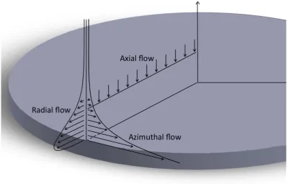
Figure 2.2 - An illustration of the three-dimensional flow on the surface of the rotating disk. ... 6
Figure 3.1 – Sketch of the disk surface, coordinate system and flow profiles. ... 27
Figure 3.2 - Velocity profiles for the f, g and h components.. ... 31
Figure 3.3 - Radial velocity profile for increasing roughness ratio. ... 34
Figure 3.4 - Azimuthal velocity profile for increasing roughness ratio. ... 34
Figure 3.5 - Axial velocity profiles for increasing roughness ratio. ... 35
Figure 3.6 - Derivative of the radial profile showing the points of inflection. ... 35
Figure 3.7 - Example of a spatial branch ... 41
Figure 4.1 - Neutral curve plot against with increasing roughness ratio. ... 43
Figure 4.2 - Instability growth rates for the neutral curve of the smooth disk. ... 46
Figure 4.3 - Neutral curve plot against with increasing roughness ratio. ... 50
Figure 4.4 - Initial azimuthal wavenumber for Type 1 lobe and Type 2 lobe ... 51
Figure 4.5 - Points of initial instability taken from neutral curves for increasing roughness ratio. ... 52
Figure 4.6 - Neutral curve plot against with increasing roughness ratio. ... 53
Figure 4.7 - Predicted initial wave angle with increasing roughness ratio ... 54
Figure 5.1 - Rotating disk facility ... 56
Figure 5.2 - Rotating disk tank set-up. ... 58
viii
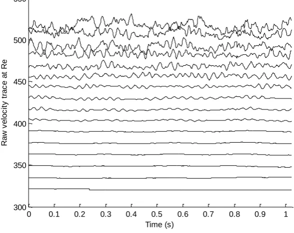
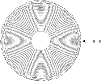
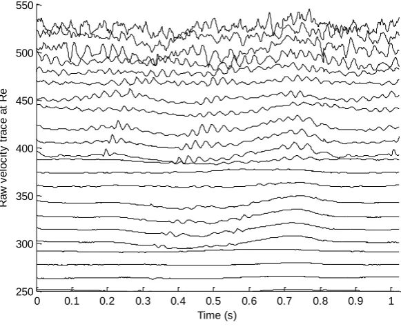
Figure 5.5 - Comparison between rough disk trace and surface function. ... 65 Figure 6.1 – Radial and azimuthal velocity profiles for disks of increasing roughness at Re = 300, Ω = 7.85. ... 72 Figure 6.2 - Comparison of raw and filtered velocity profiles. ... 74 Figure 6.3 - Radial velocity profiles for disks of increasing roughness at Re = 300, Ω = 7.85. ... 75 Figure 6.4 - Radial velocity profiles for disks of increasing roughness at Re = 400, Ω = 7.85. ... 76 Figure 6.5 - Radial velocity profiles for disks of increasing roughness at Re = 530, Ω = 7.85. ... 77 Figure 6.6 - Azimuthal velocity profiles for disks of increasing roughness at Re = 300, Ω = 7.85. ... 79 Figure 6.7 - Peak normalised, ensemble averaged traces of raw voltage signals. .... 83 Figure 6.8 - Polar plot of fluctuation data from Figure 6.7. ... 84 Figure 6.9 - Peak normalised, ensemble averaged traces of raw voltage signals. .... 85 Figure 6.10 - Peak normalised, ensemble averaged traces of raw voltage signals. .. 86 Figure 6.11 - Experimental wave angles compared against numerically derived values ... 88 Figure 6.12 - Frequency flow field for a smooth glass disk rotating at
ix
Figure 6.16 - Contour flow field for a disk rotating at rad/s. ... 95 Figure 6.17 - Vortex numbers taken from frequency contour plots ... 96 Figure 6.18 - Vortex data from Figure 6.17 plotted against non-dimensional
roughness height ... 98 Figure 6.19 - Data from Figure 6.18 after averaging with respect to the number of vortices and the non-dimensional roughness... 99 Figure 6.20 - Observed vortex number and numerical wavenumbers for both modes at various roughness ratios. ... 101 Figure 6.21 - Amplification diagram for the frequency of 16 Hz for a rough disk of ratio 0.1 rotating at 9.42 rad/s. ... 104 Figure 6.22 - Experimental neutral curve for disk rotating at 9.42 rad/s ... 105 Figure 6.23 - Neutral stability curve superimposed over frequency contour map for
disk rotating at 9.42 rad/s. ... 106 Figure 6.24 - Neutral curves for surface profile and smooth disk rotating at rad/s. ... 107 Figure 6.25 - Smooth disk neutral curves shown in Figure 6.24 with overlaid
x
xi
xii
xiii
xiv
This thesis is concerned with discovering the effect of a distributed roughness on the boundary-layer stability of a rotating disk. The investigation uses both a local, linear stability analysis and machined aluminium disks rotating in water in conjunction with a hot-film anemometer system. The stability analysis applies a sinusoidal function to the surface of the disk which mimics anisotropic roughness similar to a grooved record. The new surface is used with the governing equations in order to calculate the new mean flow profiles for the now grooved surface at a variety of roughnesses. These new flow profiles are then used in the stability analysis.
The results show that the roughness has the effect of increasing the stability of the cross-flow instability mechanism by decreasing the velocity of the radial wall jet. Conversely, increasing roughness levels cause the growth of the streamline-curvature instability mechanism, something which is probably caused by a thickening of the boundary-layer seen in the velocity profiles. These two outcomes result in a predicted switch of the dominant instability mechanism on the disk. The experimental arrangement confirms the results of the mean velocity profiles, and appears to show the appearance of the enlarged streamline-curvature instability at higher roughness levels. This instability appears as a small burst of frequencies at low Reynolds numbers centred on the numerically predicted neutral curve lobe. This burst dies down as it moves downstream, but appears to increase the amount of energy in the flow which hastens the onset of the cross-flow instability earlier than predicted. Before the emergence of this other mode at lower roughness levels, the roughness appears to delay the onset of the spiral vortices by pushing back the location of the initial cross-flow instability.
1
1
Introduction
The problem of the flow over a rotating disk has been a prominent one for many decades. The subject has garnered much interest over the years for a multitude of reasons. The fluid dynamics community find it useful due to the clean and repeatable conditions for turbulence transition, and ease in which it allows one to study a three-dimensional flow field (Lingwood 1995a). It is of interest to the aviation industry because its similarity to a swept wing boundary-layer allows easier problem formation without the more elaborate geometries (Gregory et al. 1955). Since it is relatively hard to carry out experiments on scaled swept wing models in wind tunnels, the ability to perform such experiments on a rotating disk facility instead is a great advantage (Healey 2007). Another benefit is that the disk boundary-layer has a well-known exact similarity solution for the Navier-Stokes equations which features a boundary-layer of constant thickness, making numerical calculations a lot simpler than for a swept wing (Kármán 1921). Finally, there are of course industrial processes which involve rotating disk surfaces in their own right, about which one needs to know as much as possible to maximise the effectiveness of the process. Examples include rotating impellers (Visser et al. 1999), centrifugal pumps (Adkins & Brennen 1988), and chemical vapour deposition processes (Coltrin et al. 1989).
2
Brown (2002)). Similarly, a review of the available data on the effect of roughness on the flat plate boundary-layer is presented by Dryden (2012).
More recently however, the effect of roughness on boundary-layer flow has developed a greater importance, since it was discovered that certain kinds of roughness could be beneficial to the stability of the flow and help control its structure and reduce drag (Carpenter 1997). While roughness is generally considered a scourge of a stable flow, many studies have found that carefully applied rough surfaces can delay transition to turbulence on certain geometries, and therefore studies in this area are clearly beneficial (Carrillo et al. 1996; Fransson et al. 2006).
3
4
2
Literature review
2.1 Flow structure
5
Figure 2.1 – Photo taken from Kobayashi et al. (1980), with annotations showing the three main regions of the disk; the laminar central region, the spiral vortices, and the turbulent outer region.
6
[image:21.595.112.526.174.439.2]downwards into the boundary-layer across the whole disk surface. In this way, the rotating disk flow acts like a centrifugal pump, drawing fluid down into the boundary-layer, and spinning it out from the centre of the disk outwards.
Figure 2.2 - An illustration of the three-dimensional flow on the surface of the rotating disk.
As the fluid travels through the central region of the disk, it remains laminar and steady. At some radius however, the flow will experience an instability which will develop into the distinctive, discrete spiral vortices that categorise the transitional middle region of the boundary-layer, seen clearly in Figure 2.1. The instability will be discussed later in this thesis. This unstable region eventually transitions into the final, turbulent region, which extends outwards to the edge of a finite disk, or indefinitely for an infinite disk.
7
polished disks with no protuberances can be predicted quite accurately. The radii of the regions physically move towards the centre of the disk when the rotation rate is increased, and drift further away when it decreases. This is due to the flow structure being linked, like all fluid flows, to the Reynolds number.
In most rotating disk studies, a parallel-flow approximation is applied. This approximation is used often in fluid mechanics problems as it provides simple linear equations to work with (Tollmien 1928; Schlichting 1933; Gaster 1974). In many other boundary-layer flows, the parallel flow approximation is used to account for variations of the Reynolds number in the streamwise direction due to an increasing layer thickness. However, for the disk, the thickness of the boundary-layer is constant. In the disk’s case then, the reason for applying this approximation is to make the perturbation equations separable in terms of the radius length variable, r, the azimuthal angle, θ, and t. This is achieved by ignoring any changes of the Reynolds number with radius, and replacing any instances of the radius length variable r in the governing equations by Re, thus removing any dependence on r from them. The local Reynolds number in the case of the disk is determined by the dimensional velocity, , the dimensional length scale, , and the kinematic viscosity, .
2.1
8
√
2.2
Substitute this into the Reynolds number equation to get,
√ √
2.3
Thus an increasing Reynolds number can be thought of in terms of simply moving outwards from the centre of the constantly rotating disk along the radius, or remaining at a constant radius on a disk that is speeding up.
The parallel flow approximation was shown to be valid by Cheng (1953) for boundary-layer flows provided the analysis is kept local, rather than applying globally to the whole surface. Thus the stability analysis used here will remain local in nature so as to invoke the parallel flow approximation, such as those used in studies by Malik (1981), Lingwood (1995a), Pier (2007), Garrett (2010) amongst others.
2.2 Stationary vortices
The vortices on the surface of the disk travel at different speeds in relation to the disk itself. There are many vortices which are travelling both more slowly and faster that the disk rotates, and thus these are known as travelling waves. The appearance of travelling waves on the boundary layer of the rotating disk have been well
9
rotating disk, stationary waves dominate and more likely to induce transition (Saric et al. 2003).
The waves which form the spiral vortices are travelling at the same speed and direction as the rotating disk, and so appear stationary with respect to the disk. This makes them easier to detect in experiments, and therefore this investigation will concentrate solely on stationary waves rather than travelling ones. This is mainly due to time constraints and the fact that the current experimental set-up only has one hot-film probe and so struggles to detect waves which change both spatially and temporally.
10
amplitude of 0.1% (assuming nonlinear breakdown occurs at 1%), the level of micro-roughness need only be 0.01 times the height of the displacement thickness. As Fedorov points out, these excitations are almost unavoidable and therefore will almost certainly be present on any rotating disk.
An early study by Smith (1946) done on the rotating disk boundary-layer in air, used hot wire probes to measure the wavenumber of the spiral vortices in the transition region, as well as the angle the vortices make with the radius. It was found that at a certain radius in the transition region, there were approximately 32 oscillations for every rotation of the disk, at an angle of 14°. The seminal study by Gregory et al. (1955) discovered that these values were a constant in the rotating disk system, as the angle was found to be 14° and 13°18’ from experimental and numerical observations respectively. They also discovered that the number of stationary spiral vortices in the central section was also a repeatable value, regardless of disk size, speed or fluid medium. Using a combination of china-clay visualisation and frequency data taken from acoustic microphones, they counted a total of between 28 and 31 stationary vortices on the disk surface. These values for the angle and number of vortices have since been confirmed by many studies since (Fedorov et al. 1976; Kobayashi et al. 1980; Kohama 1984; Wilkinson & Malik 1985) and have been taken as standard for the smooth disk flow.
2.3 Instabilities
11
top of the local mean flow, and see what these disturbances do as they flow downstream, or as time progresses. If they dissipate, then the flow is damped and stable at that point. However, if the perturbations grow, then the flow at that point is unstable.
There are two ways in which an unstable disturbance can affect the flow. Either the disturbance grows as it moves downstream; in which case it can only affect areas of the boundary layer downstream from the disturbance inception point, which is called a convective instability, or the disturbance remains fixed spatially, but grows temporally at this radial location to affect the flow around the inception point, including flow upstream. This is known as an absolute instability. The rotating disk boundary layer is known to include both types of instability, after Lingwood (1995a; 1996) proved the existence of the absolute instability in the boundary layer both theoretically and experimentally.
An unstable laminar flow is a precursor to transition to a turbulent flow. When performing a stability analysis, one can choose to explore the evolution of the perturbation as it develops in space downstream, which is known as a spatial analysis, or as it stays in place and grow over time, in which case it is known as a temporal analysis. In order to discover the existence and location of the absolute instability, Lingwood used a spatio-temporal analysis which is a combination of the two, as neither one of the former methods were sufficient for the rotating disk boundary layer.
12
disturbances. The points of instability can be plotted against a number of other variables such as azimuthal wavenumber or waveangle to generate neutral stability curves which help to visualise how stable a flow is overall. This visual overview helps to compare the potential stability of different flow situations. Note that a linear stability analysis cannot predict or explain any aspects of turbulence following transition, as this part of the flow necessarily contains nonlinear effects. In order to compare the numerical results with experimental data, an attempt will be made to keep our experimental boundary-layer in the linear regime by using only transitional roughness levels, for which a definition is given in Chapter 5.2.
13
experimentally to occur at anywhere from Re = 294-377 (Kobayashi et al. 1980; Malik et al. 1981).
The second known instability is the streamline-curvature instability. Through performing calculations with the Orr-Sommerfeld equations, which are essentially just stability analyses with Coriolis and streamline-curvature terms removed, many studies have found that this ‘Type 2’ instability does not appear. This is because the streamline-curvature instability is thought to be caused by a balance between viscous and Coriolis effects (Hall 1986), and therefore it makes sense that all signs of it disappear in stability results when the Coriolis and streamline-curvature terms are excluded (Lingwood 1995a) and at high Reynolds numbers (Lilly 1966). Itoh (1996) found that the strength of the streamline-curvature instability could be described using the parameter κ, which is defined as the ratio between the boundary-layer thickness and the radius of the curved streamlines. By varying the value of this parameter, it was shown that the critical Reynolds number of this instability increases to infinity as a curvature term decreased to zero, thus concluding that the instability was caused by the curved streamlines of the flow.
14
direction to the spiral vortices) with a wavenumber of around 14-16 (Fedorov et al. 1976). These values have been confirmed numerically by Faller (1991) and Malik (1986) for the rotating disk, and by Tatro and Mollo-Christensen (1967) for the Ekman layer, which is similar to the rotating disk flow except the fluid is experiencing a solid body rotation almost equal to the velocity of the disk.
2.4 Transition
The point at which the spiral vortices break down into full turbulence is consistent and repeatable, in contrast to the more complicated pipe or flat plate transition points where transition into turbulence can vary enormously depending on many factors. Because of this repeatability, many experimentalists have been trying to pin-point its exact location. Many studies using visual methods such as china-clay or naphthalene, or data collection methods such as hot-wire or acoustical probes have narrowed the region of transition to a Reynolds number of between Re = 490 and 540 (A table of collated results can be found in Healey (2010)). It was discovered by Lingwood (1995a), that the repeatability of this location could well be due to an absolute instability occurring at Re = 510 (although this was later corrected to be 507.3) in numerical calculations and between Re = 504 and 514 found in experiments. Due to this absolute instability appearing within the region of measured transitional Reynolds numbers, Lingwood postulated that this leads to an unbounded linear response at these radii, which promotes transition around this Reynolds number.
15
points, but Healey (2010) suggests another possibility; Healey noticed that due to the disks used in each experiment being of varying radii, they each had a different Reynolds number for their edge. He hypothesised that the edge Reynolds number could have an effect on the transition point, and that upstream effects from the edge could be stabilising the flow beyond what should be possible. He finds a correlation between the edge Reynolds number and the transition Reynolds number that could explain the transition numbers higher than expected from previous experiments. Imayama et al. (2013) performs a study specifically designed to test Healey’s theory, and finds there to be only very weak correlation between the transition Reynolds number and the proximity to the edge of the disk. They hypothesise that the actual reason for large variations in transitional points are again down to differences in judging when transition has occurred.
2.5 Routes to turbulence
16
If no triad couplings are formed, stationary waves are formed as usual by the cross-flow instability and can lead to transition in two ways. Firstly, if they are of high amplitude they will form high frequency secondary instabilities which grow and cause rapid transition to turbulence. Balachandar (1992) performed a Floquet analysis for the 3D boundary-layer on a rotating disk and calculates the secondary instabilities by first working out the primary disturbance before adding it to the mean flow as a superposition and working out the secondary disturbance from this. He found that the critical amplitude for the primary disturbances was approximately 9%, above which the secondary instabilities would form and grow rapidly. These secondary disturbances took the form of counter-rotating vortices which occur at an angle from the primary spiral vortices, which had been seen a few years before by Kohama (1984) using smoke visualisations.
17
stable. Thus the role of the absolute instability on turbulent transition is still an uncertain one.
2.6 Roughness
Although theoretical studies often assume otherwise, surfaces in the real world cannot be completely smooth. In the field of fluid dynamics, small amounts of roughness on a micron-scale can have a large effect on the structure of a flow, and neglecting this roughness can result in some large discrepancies between theory and experiments. For this reason it is important to consider the flow over surfaces with roughness added, although due to the sheer variety of different types of roughness, this can often be very difficult. Roughness elements can differ in size, distribution and shape which all have different effects on the fluid and two experiments with seemingly similar roughness levels will display completely different flow characteristics.
18
From this it can be ascertained that as long as the roughness elements remain within the boundary-layer, the pressure drop along the pipe should be equal to that of a pipe with smooth walls. Clearly pipe flow differs greatly from rotating disk flow, but an effort to keep the roughness protrusions within the boundary-layer for the disk will be made in an attempt to keep pressure gradients to a minimum.
Schlichting and Gersten (2004) use the regions present in the theory of the ‘universal law of the wall’ to describe three roughness regimes. For roughness below a certain level, they use the term hydraulically smooth to refer to a wall surface where the boundary-layer is not affected by the roughness. They also describe a regime where the roughness elements are so large they take up all of the wall boundary-layer, creating pressure forces which dominate the flow. They call this region fully rough. Finally, in between these two they define a regime known as
the transition region which contains roughness elements large enough to affect the
flow, but not so great that they create large pressure forces. From Nikuradse’s findings above, in order to keep the protrusions within the boundary-layer the roughness used in this study will have to fall within the transitional region of roughness. Details on how this was achieved are found in Chapter 5.2.
19
simplified flow and easily identifiable structures, and so are often used to mimic simple roughness. The third class is distributed roughness which covers the whole surface of the study, such as sandpaper or a corrugated surface.
Sandpaper is a common choice for creating rough surfaces (Leventhal & Reshotko 1981; Corke et al. 1986; Watanabe 1987), but aside from their average grain size, two sets of sandpaper will differ greatly in terms of height, pitch and distribution of sand grains. In addition to this, attempting to model a randomly rough surface such as sandpaper numerically becomes too difficult. For these reason, the roughness chosen for this study will be three-dimensional and distributed in nature, to try and match physical roughnesses found in real applications, yet will be simple enough to model numerically and produce experimental results which can be compared with others.
2.7 Boundary-layer control techniques
20
Active flow control are methods which require an energy input to work, such as the suction method mentioned above and in later studies (Pfenninger 1946), or surface cooling (Wazzan et al. 1968). These flow control techniques work by forcing the second derivative of the velocity profile near the surface to be more negative (Reshotko 1984). The downsides to these in terms of use on aeroplanes are that they may possibly use as much energy to work as they would save through drag reductions. Similarly, they also require extra weight to be added to the aircraft which would negate the benefit of any fuel saved.
The second group of control methods are the passive type, by which no energy input is required to have the control effect. The method usually requires modifying the surface in some way such as adding a compliant layer (Carpenter et al. 2000) or the adding of leading edge ‘tubercles’ or scallops (Fish & Lauder 2006). Another popular technique is the modification of adding a rough surface.
2.8 Roughness as a control mechanism
The technique of using a rough surface to control the transition to turbulence has been widely considered in recent years. For example, airline component manufacturer Lufthansa Technik are experimenting with adding sharkskin-like riblets to the surface of the fuselage and wings of Lufthansa planes in an attempt to reduce drag and decrease fuel consumption by up to 1% (Lufthansa-Technik 2013). Understanding how such roughness works to delay the transition point is thus very important and there are many studies which work towards this understanding.
21
surface, and gauge how the flow reacts to this on a local scale. Many studies on the rotating disk in the past have usually dealt with these small roughness elements acting as a point source rather than a distributed roughness covering the whole disk surface (Jarre et al. 1996a; Wilkinson & Malik 1985; Mack 1985). The studies find that the spiral instabilities emanate from small point sources of roughness on the disk, whether they are naturally occurring or intentionally placed.
This method allows the authors to trip the flow and creates a localised, amplified instability in order to study it. In this case, the actual roughness used is not important; the same effect can be gained by introducing a puff of fluid into the boundary-layer instead (Lingwood 1996), although this latter study excites all frequencies rather than just stationary ones. However, the roughness element in the above cases is simply used as a controlled, repeatable path to a pure transition. Essentially, this is not full roughness, and so any effects to the boundary-layer will not be indicative of how the flow will react to a fully rough disk, which is the aim of this thesis.
22
thickening of the boundary-layer and reduction in the flow velocities because of this (Miklavcic & Wang 2004).
Zoueshtiagh (2003) measured the transitional Reynolds number for the flow over a rough rotating disk submerged in water. Roughness levels of 170μm, 335μm and 1325μm were achieved by attaching quartz granules of differing diameters to the surface of smooth glass disks. It was found that there was no noticeable effect on the transition location until a threshold level of roughness was reached, upon which point, the critical Reynolds number fell sharply. However, at some of the higher rotation rates, the method of determining the transition point (via flow visualisation) was up to 20% in error. Therefore, there could have been effects unseen for the lower levels of roughness.
To make the process of modelling and quantifying roughness easier, many studies use riblets, or patterns of roughness in a variety of shapes. Configurations such as V-shapes (Wang et al. 2000), rectangles (Elsamni et al. 2007), triangular grooves (Baron & Quadrio 1993) have all been tried with varying degrees of success.
23
One study by Fransson et al. (2006) found they could delay transition on a flat plate in a wind tunnel by using cylindrical roughness elements to induce a streaky base flow. This helps to reduce the exponential growth of Tollmien-Schlichting waves and shift the transition location downstream. Similarly, transition delays have been seen for swept wing boundary-layer flow. Radeztsky (1999) used random, natural-surface roughness to delay transition from 48% to 77% chord on a swept wing, while Reibert (1996) and Saric (1998) both used periodic roughness arrays to achieve similar results. More recently, Hosseini et al. (2013) performed direct numerical simulations in order to confirm the study by Saric, albeit with a more complex disturbance field, and produced results in agreement with Saric. They found that the leading edge cylindrical roughness elements delayed transition from 45% to 60% chord by damping the most unstable cross-flow mode as well as the secondary instabilities.
An attempt to mimic the three-dimensional form of shark scales and its role in reducing drag found that 3D riblets did reduce the drag by 6.85%, but this was less than the 9% achieved for the 2D case (Bechert et al. 2000). Manufacturing these complicated 3D riblets however, turned out to be a formidable undertaking, and so easier ways of creating roughness patterns are often sought.
24
flow of the boundary-layer (Watanabe et al. 2007). They also found that the spiral grooves suppressed the generation of local vortices, and modified the boundary-layer velocity profiles by decreasing the flow velocities in both the azimuthal and radial directions.
25
3
Numerical formulation
To formulate the stability equations for the rough, rotating disk, the approach taken by Lingwood (1995a) and Garrett (2002) is adopted, incorporating a method set by Yoon et al. (2007) to control the surface roughness. The first step will be to add the rough surface to the disk geometry by replacing the standard flat radial axis with that described by a simple function which changes only with the radial coordinate. With this new geometry, the next step will be to calculate the governing equations which describe the mean flow components over this new disk and solve them to obtain the three-dimensional velocity profiles for disks with distributed roughness. Yoon et al. (2007) calculated mean flow profiles for their new disk surface geometry, but only looked at one roughness level at changing Rossby numbers. A similar method is used here to look at how the mean flow profiles change over a range of surface roughnesses. These mean flow profiles will then be used as a basis to conduct the linear stability analysis, in which the behaviour of small perturbations added to the mean flow are studied as they evolve downstream. This will be done using the framework and stability code developed by Lingwood mentioned previously, through which the perturbation equations are formed and then solved to determine the stability of the disk boundary-layer using these new flow profiles.
26
to small changes in the mean profile. Hence performing stability calculations on the distorted theoretical flow is likely a valid technique to use.
3.1 Steady flow profiles
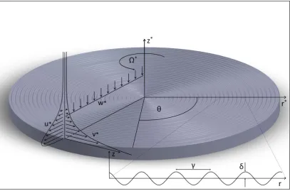
The geometry used is similar to many previous rotating disk studies; an infinite disk rotating in an incompressible, Newtonian fluid is presented, and described using a cylindrical coordinate system. The radial coordinate is taken to be and the azimuthal coordinate to be . The disk rotates at a constant angular velocity around the axial direction (see Figure 3.1 for a diagram of the system). For this problem, a fixed frame of reference in which the rotating disk rotates is used, in contrast to other studies where the frame of reference rotates with the disk itself. Because of this approach, no Coriolis terms will appear in the governing equations, which simplify them somewhat. The steady flow components in these directions are , and . The fluid itself has a pressure , density and kinematic viscosity . All dimensional quantities are indicated by asterisks. These dimensional quantities are scaled by a characteristic length-scale given by the boundary-layer thickness, √ ⁄ a velocity scale given by and a pressure scale given by .
27
Figure 3.1 – Sketch of the disk surface, coordinate system and flow profiles.
In order to add a distributed roughness to the disk, the approach of Yoon et al. is to describe the surface of the disk as a function such as ⁄ where is the amplitude and is the wavelength of the surface variation resulting in a ‘wavy’ surface such as in Figure 3.1. This function can of course be non-dimensionalised using the above scales to get
( ) 3.1
with and being the non-dimensional amplitude and wavelength parameters respectively. These are the control parameters which allow the amount of roughness on the surface of the disk to be varied, and it is useful to refer to them in terms of the ratio between the two, i.e. the roughness ratio ⁄ .
28
theorem (Prandtl 1938) which is a method to transform a complex geometry onto a simpler one, without having to change the boundary conditions. This is done by switching to a new coordinate system where and similarly transforming all velocity components
3.2
with the prime representing differentiation with respect to . For the current study, we are only interested in situations where the disk is rotating rapidly enough to form a thin boundary-layer. In other words it is required that . Thus this boundary-layer assumption can be enforced by setting
̃ ⁄ 3.3
Finally, variables closely related to von Kármán similarity variables to describe the velocity components are introduced
̃ 3.4
In order to form the new governing equations, we first take the non-dimensionalised, cylindrical Navier Stokes equations and apply the transformations from Equation 3.2 and the boundary-layer assumptions before substituting in the variables from Equation 3.4. The result is the set of partial differential equations
3.5
(
) ( )
29
( )
3.7
subject to the boundary conditions
3.8
where the flow at the disk surface is subject to no-slip conditions and there is quiescent fluid far from the disk. In creating Equations 3.5-3.7, we have invoked the assumption that there is no pressure gradient in the radial direction, or ⁄ . This is considered valid as long as the roughness ratio remains small, according to Le Palec et al. (1990). The justification is that if the surface roughness ratio is small, there is less variation from peaks to trough of the sine function that could result in a difference of pressure in between. The equations reduce to the familiar von Kármán equations as the roughness function on the disk becomes flat i.e. as .
These partial differential equations can be solved easily using the commercial NAG routine D03PEF. The routine reduces the PDEs to a system of ordinary differential equations in using the method of lines. This routine has been used successfully on a number of occasions by Garrett and co-workers (Garrett & Peake 2002; Garrett et al. 2010; Samad & Garrett 2010; Barrow & Garrett 2013).
30
equations using the central difference method. The points for this method are taken to be at the four corners of a box, hence the name. The equations are then linearized, removing higher order terms, before being solved by a backwards difference method.
The equations are solved at an initial radius using the backwards difference method for 100 points between the surface of the disk and a height of . This solution is then used to solve the next iteration at the next radius as the routine moves outwards.
The initial solution at is found by using the series solution method used by
Banks (1965). The method replaces the velocity components in the PDEs ( ) with series expansions in terms of and because is small we can reject higher
order terms and simply look at leading order terms. As it turns out, using the series expansion method results in the initial solution at being the original von Kármán disk profile for all , and so the initial input for the system at is simply the smooth von Kármán profiles.
31
effectiveness of this averaging and the whole mean flow method will be tested by experimental verification in Chapter 6.1.
3.1.1 Code validation
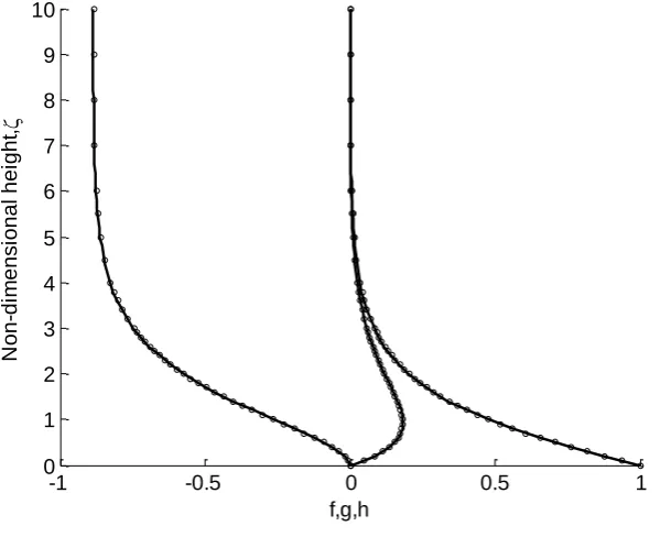
Figure 3.2 - Velocity profiles for the f, g and h components. (-) shows ‘smooth’ results from the D03PEF routine with δ = 0, γ = 1. (o) shows results taken from (Owen & Rogers 1989).
In order to validate the results generated by the NAG routines, the velocity profiles for the smooth case where and can be compared to previously generated profiles. As can be seen in Figure 3.2, the velocity profiles for all three coordinates (solid lines) are compared against profiles taken from Owen and Rogers (1989) (circles) for and . For all three velocity components, the smooth flows are similar.
3.1.2 Results
Figures 3.3-3.5 show the three velocity components for disks with varying roughness. The results are taken at an arbitrary radius of and averaged over one wavelength, since the solution is independent of radial location. There is a
-1 -0.5 0 0.5 1
[image:46.595.165.470.184.428.2]32
noticeable effect as the roughness is increased from a smooth disk ⁄ through to ⁄ . For the radial component, the effect is to decrease the velocity of the wall jet and increase the overall thickness of the boundary-layer. A similar effect was seen experimentally on a flat plate boundary-layer by Leventhal and Reshotko (1981) where sandpaper roughness caused a thickening of the Blasius (flat plate) boundary-layer, and also by Baron and Quadrio (1993) who saw a thickening of the viscous sublayer in turbulent flow over triangular riblets. The decrease in velocity makes physical sense since the friction of the roughness would act to hold back the base of the wall jet. Lessen and Gangwani (1976) plotted the disturbed velocity profiles of the flow over a flat plate with a wavy surface and found there to be a mean backflow for the streamwise profile caused by the zero flow effect at the crests and valleys of the wall. It could be that a similar result causes a reduction in the wall jet by adding a small backflow element to the forward facing jet.
For the radial profiles, the inflectional point on the radial profile is shifted upwards as can be seen more clearly in Figure 3.6. This figure simply plots the first derivative of the radial profile ( ⁄ ) for each roughness, so that the height of the inflection point is more visible.
33
inflection point begins to fall again. However, it is thought that this result is due to limitations in the code rather than an indication of how the flow might behave. According to Le Palec (1990), the assumption of an unchanging pressure difference across the sinusoidal profile can only be justified for mild roughness, i.e. small ⁄ . For this study therefore it was decided to keep ⁄ as an upper limit on the amount of roughness.
In the study by Lessen and Gangwani (1976), an inflection point was induced in the mean flow profile of the flat plate with the addition of the wavy surface. There was no comparison between increasing levels of roughness and position of the inflection point in their paper however, so it is not known if this effect is related to the upward trend seen in Figure 3.6 or if it is simply a consequence of the slower wall jet and thickened boundary-layer.
34
Figure 3.3 - Radial velocity profile for increasing roughness ratio.
Figure 3.4 - Azimuthal velocity profile for increasing roughness ratio.
0 0.05 0.1 0.15 0.2
0 2 4 6 8 10 12 14 16 18 20
Radial velocity, f
N o n -d im e n si o n a l h e ig h t,
/=0.0
/=0.08
/=0.12
/=0.16
/=0.2
0 0.2 0.4 0.6 0.8 1
0 2 4 6 8 10 12 14 16 18 20
Azimuthal velocity, g
N o n -d im e n si o n a l h e ig h t,
/=0.0
/=0.08
/=0.12
/=0.16
35
Figure 3.5 - Axial velocity profiles for increasing roughness ratio.
Figure 3.6 - Derivative of the radial profile showing the points of inflection.
-1.40 -1.2 -1 -0.8 -0.6 -0.4 -0.2 0 2 4 6 8 10 12 14 16 18 20
Axial velocity, h
N o n -d im e n si o n a l h e ig h t,
/=0.0
/=0.08
/=0.12
/=0.16
/=0.2
-0.10 0 0.1 0.2 0.3 0.4 0.5 0.6 1 2 3 4 5 6 7 8 9 10
Radial velocity derivative, f'
N o n -d im e n si o n a l h e ig h t,
/=0.0
/=0.08
/=0.12
/=0.16
36
3.2 Deriving the perturbation equations
Once the steady state velocity profiles for the sinusoidal rough surface are found, they can be used to predict the stability of the flow for the range of values of
. The method in this section follows closely the method used by Lingwood (1995b) and Garrett (2002). First, the perturbation equations which will be used to track the flow’s stability must be derived. Infinitesimally small perturbing quantities are added to the averaged steady flow profiles which are then substituted into the boundary-layer equations. We will use upper-case barred symbols for the perturbed flow components, and lower-case hatted symbols for the perturbing quantities for clarity. The steady state components are as before.
̅ ̅ ̅ ̅ ̂ ̂ ̂ ̂ 3.9 The perturbations take the normal mode form
̂ ̂ ̂ ̂ 3.10
37
Due to the transformation carried out in Equation 3.2, the computed velocity components do not currently compare to the physical domain. The radial and azimuthal components have not changed but the axial flow component is affected by the wavy floor and so a transformation such as the following may be necessary
̃ 3.11
However, looking at Equation 3.11 it is obvious that averaged over the length of one wavelength reduces to zero, and thus W and ̃ are approximately the same. Therefore as long as any future surface function remains oscillatory, any dependency on radial location can be averaged out.
Replacing the velocity components in the cylindrical, dimensionless, steady Navier Stokes equations with Equations 3.9 and 3.10 and then simplifying gives us the following equations: ̅ ̅ 3.12 ̅ ̅ ̅ 3.13 ̅ ̅ 3.14
38
In the above, the mean flows have been subtracted and the equations have been linearized to remove terms of higher order, since the perturbations are already very small and so any terms of higher order would be negligible. is locally constant and as such does not change with , hence we have replaced all instances of radial distance with , while ̅ ⁄ . The prime in Equations 3.12-3.15 indicates differentiation with respect to the axial coordinate .
We can write the perturbation Equations 3.12-3.15 in a different way by using a set of transformed variables taken from Lingwood (1995a).
(
) ̅
3.16
(
) ̅
3.17
3.18
3.19
(
) ̅
3.20
(
) ̅
3.21
This allows us to express the perturbations as the following six ordinary differential equations:
3.22
(( ) ̅ ) ( ̅
)
(( ̅ ) ( ̅ ) )
39
[ ]
3.24
([ ̅ ] ( ̅ ) ) [
]
[ ]
3.25
3.26
[( ̅ ) ̅ ] [( ̅ ̅ ) ( ̅ ̅ ) ]
̅
3.27
It is noted that these equations are identical to those derived by Lingwood. The result of this formulation is that the addition of roughness only changes the form of the steady flow and not the perturbation equations.
3.3 Solving the perturbation equations
In order to solve the eigenvalue problem posed by Equations 3.22-3.27, we set out the boundary conditions as follows, which are now in a rotating frame of reference
3.28
where . This ensures that the disturbances die out after leaving the boundary-layer. The problem needs to be solved for certain combinations of values of for inputs of the parameters . Hence we form the dispersion relation:
3.29
Runge-40
Kutta integrator with Gram-Schmidt orthonormalization and a Newton-Raphson linear search procedure.
For user determined values of the Reynolds number and roughness levels and for a starting value of the code increments through increasing values of and calculates and at each point. As mentioned previously, since we are only interested in the growth of the perturbations downstream in the radial direction, we can set . This disallows any growth in the azimuthal direction and provides an axisymmetric amplitude distribution.
Since we are assuming that the spiral vortices we are looking for are stationary, we can set the frequency of the vortices to be equal to the frequency of the disk speed, i.e. they are stationary with respect to the disk and therefore we ensure .
41
Figure 3.7 - Example of a spatial branch taken at Re = 570 for a roughness ratio of ⁄ . Circles indicate points of neutral stability.
Figure 3.7 shows an example branch developing in the α-plane for a certain Reynolds number. The code tracks the branch as it develops with increasing values of βr from left to right. Initially at low the flow is stable and all perturbations will
be damped. Then as the branch drops below the x-axis, the perturbations become unstable and excited. The growth rate of these disturbances is linked to the distance they fall below the x-axis. In other words, the more negative becomes, the higher the growth rate of the excited perturbation. The points at which the branch crosses the x-axis are important as these display the limits of the unstable region; the neutral stability points.
Whilst keeping the roughness variables the same, the Reynolds number can be incremented and the eigenvalue problem solved again to find the zero-growth neutral stability points at successive radii. In this way a neutral stability curve can
0 0.1 0.2 0.3 0.4 0.5 0.6 0.7
-0.06 -0.04 -0.02 0 0.02 0.04 0.06 0.08
Re = 570
r
42
43
4
Numerical results
4.1 Neutral curves
Neutral curves are produced for a range of different roughness ratios for a disk with a sinusoidal roughness pattern, and the comparisons between them are presented here. As is standard for neutral curve plots, the Reynolds number of the flow is plotted against different variables, namely , and the angle of disturbance in order to see the range of stability that the flow should have.
Figure 4.1 - Neutral curve plot against with increasing roughness ratio.
Figure 4.1 shows the stability curve for the rough rotating disk with increasing levels of roughness ratio. The ratio ⁄ represents a smooth disk surface, and comparisons between the shape of this curve and curves from other studies are positive. It is known that ‘upper’ lobe of this curve is caused by the Type 1, or cross-flow instability in the boundary-layer cross-flow, while the ‘lower’ lobe is caused by Type
100 200 300 400 500 600 700 0
0.1 0.2 0.3 0.4 0.5 0.6 0.7
Re
r
/ = 0.0
/ = 0.1
/ = 0.2
44
2, or the streamline-curvature instability (Malik 1986). For the smooth case, it can be seen that the upper lobe is much larger, and first occurs at a much lower Reynolds number than the lower lobe. From this it can be ascertained that for smooth disk flow, and for low conditions of roughness, any unstable flow is most likely caused by the cross-flow instability as the flow moves outwards with increasing radius. In this case, the onset of the cross-flow instability is found at about Re = 281±1 for the smooth disk, which compares favourably to the values of 285 and 287 obtained by Malik (1986) and Mack (1985) respectively; the small discrepancy is most likely due to truncation and rounding errors.
As the ratio of the roughness level is increased however, some changes become apparent in the stability of the flow. Firstly, the overall size of the area of instability decreases, becoming thinner and suggesting an overall stabilising effect of the roughness. Secondly, the upper lobe decreases in size significantly, whilst shifting to higher Re. Lastly, the lower Type 2 lobe begins to increase in size, growing in both width and length and shifting upstream to lower Reynolds number.
The reduction of the main cross-flow instability lobe as roughness is increased can be explained by the decrease in the mean flow velocity of the radial wall jet seen in Chapter 3.1. This reduction in the strength of the cross-flow element of the boundary-layer would explain the stabilisation of that instability, as the mean velocity and vorticity of the flow passing through the inflection point will be less, and so the tendency to become unstable will also be reduced.
45
parameter ⁄ derived by Itoh (1996) to describe the effect of the streamline-curvature, we see that it is dependent on two factors; the radius of the curved streamlines, and the thickness of the boundary-layer. The streamline radius is simply the local radius of the resultant velocity streamlines. As the wall jet velocity decreases and the azimuthal velocity remains approximately steady, the streamlines of the resultant flow become a tighter curve with a smaller radius. In addition to this, in Chapter 3.1 a thickening of the boundary-layer was observed as roughness was increased, thus increasing the value of . Together, these two changes increase the streamline-curvature parameter . Hence, it can be seen that as the mean velocity profiles experience this thickening, and the streamlines gain a tighter radius of curvature, the result is a growth in the streamline-curvature instability mode.
These changes in the neutral curves become significant at between ratios of 0.1 and 0.2 where the unstable mode at the lowest Re switches from the upper lobe to the lower lobe. In fact, this switch in the location of the critical Re occurs at approximately ⁄ . This could signify a switch in the dominant mode, although more crucially one must look at growth rates of each instability mode rather than just simply where the flow becomes unstable.
4.2 Instability growth rates
46
plane of the neutral curves in Figure 4.1. This approach is consistent with that taken by Garrett (2010)
For the smooth disk case shown in Figure 4.2a, as expected, the Type 1 cross-flow instability growth rate is much larger than the Type 2 streamline-curvature instability. In fact, for the smooth case, the growth rate of the lower lobe (to the left of the 3D plot) is barely visible, which conforms to the widely held view that the cross-flow instability dominates the flow over a smooth disk at all radii for stationary modes.
Figure 4.2 - Instability growth rates for the neutral curve of the smooth disk a) ⁄ and rough disks b) ⁄ , c) ⁄ , d) ⁄ .
If the roughness ratio is increased to 0.12, the point at which the modes switch in Figure 4.1, we see once again the growth of the streamline-curvature mode and the reduction of the cross-flow but it is clear from Figure 4.2b that the growth rate of
a) b)
47
the latter mode still dominates. Any Type 2 instability that forms will quickly be dominated by the growth rate of the Type 1 instability many times larger than it. Increasing the roughness ratio further to 0.2 (Figure 4.2c) sees an additional reduction in the growth rate of the cross-flow mode and for a short range of Reynolds numbers, the growth of both instabilities is approximately equal. (The cross-flow eventually dominates after Re=550, but we know from previous studies that this region is likely to be both turbulent and nonlinear in nature, and thus the linear stability behaviour at that point is moot). This level of roughness therefore could be a second possible switching point in the development of the rough boundary-layer flow, as it details the critical roughness needed for the growth rate of the Type 2 instability to overcome the Type 1. For roughnesses above this critical level, such as in Figure 4.2d, it can be seen that the streamline-curvature mode both occurs further upstream and dominates in terms of growth rate as Re increases.
48
most likely that this reduction in the cross-flow mode is caused by the roughness influencing the height of the inflection point in the boundary-layer and reducing the velocity of the wall jet. This conclusion is based on how the radial profile and the inflection point are so closely linked with the formation of the cross-flow instability in the literature.
4.3 Azimuthal wavenumber
Another variable that can be investigated in terms of the neutral stability is the azimuthal wavenumber which is the real part of the azimuthal quantity ̅ used in Equations 3.12-3.15. The azimuthal wavenumber is a value that can be directly compared to the physical quantity of the number of vortices seen around the disk. As mentioned in Chapter 2.2, the general consensus for the experimental smooth disk is a value of between 28-32 fully developed spiral vortices. For numerical studies, values as high as 113 have been seen (Gregory et al. 1955), but this value was calculated without considering viscous, Coriolis and streamline-curvature effects. In Chapter 3.2 the parameter was replaced in Equations 3.12-3.15, and so to convert the azimuthal wavenumber back to the physical number of vortices, it needs to be multiplied by the Reynolds number at which the value was taken.
4.1
49
new interesting effect. The vortex number at which instability first occurs noticeably decreases as well. For the smooth case, the instability first occurs at Re = 281 with a vortex number of approximately 22, which is consistent with previous smooth disk stability calculations (Malik 1986). It is worth pointing out that this value for the number of vortices is not directly comparable to those seen in experiments, since this is the initial value for the vortex number, at the first point of instability. In experiments, the spiral vortices generally are not visible until further downstream when they have increased in number through bifurcations. Jarre et al. (1996b) note that the discrepancy between the wavenumber of 22 seen in the numerical curves and their experimental observations of 32 could be caused by the nonlinear effects present on the disk, which are not taken into account with the linear stability study. This idea is supported by the earlier work of Wilkinson and Malik (1985), who kept nonlinear effects to a minimum during their experimentsby using a flow control panel to draw away any turbulent forcing. With these low turbulence levels, they managed to record the exact number of vortices at each radius of the disk. In Figure 6 of their paper the number of vortices increases sharply from the critical location of Re=289 to reach a value of approximately 23 vortices, before then slowly increasing through vortex bifurcations to the familiar value of 32.
50
0.2. For the lower lobe, the reduction in vortex number is even more noticeable; a reduction from 21 for the smooth case, to 11 for a roughness ratio of 0.2.
It was first noticed by Stuart (1955) and confirmed by Malik (1986) that the wavenumber is greatly susceptible to changes in viscosity. Malik notes that the wavenumber at high Reynolds numbers, where viscous effects are negligible, differs greatly from the wavenumber at the critical point. Because of this, it makes sense that the viscous mode is affected to a higher degree than the inviscid when subjected to increasing roughness.
Figure 4.3 - Neutral curve plot against with increasing roughness ratio.
This reduction in initial vortex number shows some similarity to the reduction of spiral vortices seen by Watanabe et al. (1993) as they increased the size of the roughness on their disk. Because of the link between critical wavenumber and number of developed spiral vortices, it seems likely that this stability result is the
200 300 400 500 600 700
0 10 20 30 40 50 60 70 80 90 100
Re
/ = 0.0
/ = 0.08
/ = 0.12
/ = 0.16
51
cause of the effects seen by Watanabe, and will be confirmed with experiments in Chapter 6.
The values of the initial vortex numbers from the curves in Figure 4.3 can be recorded along with the values taken from other curves for ratios not shown here.
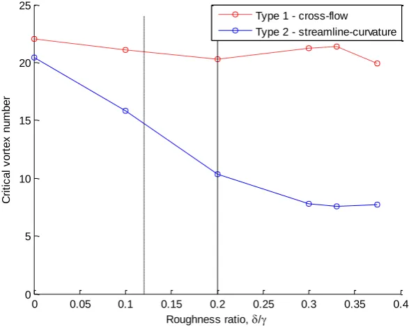
Figure 4.4 - Initial azimuthal wavenumber for Type 1 lobe and Type 2 lobe. Vertical lines indicate possible mode switch locations.
From Figure 4.4 we can see that the predicted trend of the number of azimuthal vortices is indeed downwards with increasing roughness ratio, with the slope of the Type 2 lobe greater than the Type 1 lobe. Because of this difference in slope, one might expect that if there was a switch of the dominant modes, one of the observable changes in the experimental data could be a change in the slope of spiral vortex number too, providing of course that the Type 2 mode still appear as vortices once dominant.
0 0.05 0.1 0.15 0.2 0.25 0.3 0.35 0.4 0 5 10 15 20 25
Roughness ratio, /
C ri ti c a l v o rt e x n u m b e r
Type 1 - cross-flow
[image:66.595.168.462.225.460.2]52
The possible switch locations have been added to the plot; the point at which the critical Re for the Type 2 lobe overtakes Type 1 ( ⁄ ), and the point at which the growth rate of the Type 2 lobe dominates Type 1 ( ⁄ ). At one of these points, one might expect to see a sudden drop in the number of observed experimental spiral vortices as the mode switches from the upper slope to the lower.
It is also pertinent to look at the critical Reynolds number at which the instabilities first form for each roughness ratio. This will give us the range of Reynolds numbers for which one would expect to see instabilities first forming in the experimental data.
Figure 4.5 - Points of initial instability taken from neutral curves for increasing roughness ratio.
Figure 4.5 shows clearly the point at which the switch between the two lobes for the critical Reynolds numbers occurs. The markers show the decreasing Reynolds numbers for the initial cross-flow instability location and the increasing location of
0 0.05 0.1 0.15 0.2 0.25 0.3 0.35
150 200 250 300 350 400 450 500 550 600 650
Roughness ratio, /
C ri ti c a l R e y n o ld s n u m b e r
Type 1 - cross-flow
53
the streamline-curvature instability. These curves are another way in which one can look for mode switches, by comparing them to the experimentally obtained points of initial instability and looking for any change in the behaviour as the roughness is increased. The results of this will be discussed in Chapter 6.6.
An important point to note is that if there is no mode switch to the streamline-curvature mode, and instabilities continue to be caused solely by the cross-flow mode, then the point of initial instability should, in theory, be delayed by increasing the amount of roughness. This in turn could have the effect of delaying transition to turbulence.
4.4 Wave angle
Figure 4.6 - Neutral curve plot against with increasing roughness ratio.
The range of neutral stability can be viewed through one other parameter plane, the angle of propagation of the disturbances, or wave angle . This parameter is
100 200 300 400 500 600 700 8
10 12 14 16 18 20 22 24 26
Re
/ = 0.0
/ = 0.08
/ = 0.12
/ = 0.16
54
simply the angle of the resultant wave with respect to the radial axis, and can be calculated simply using the formula
( ̅) 4.2
Figure 4.6 shows the relationship of changing neutral curve with increasing roughness ratio. Note that for the wave angle neutral curve, the lobe representing the cross-flow instability is on the bottom, while the streamline-curvature lobe is on the top. The situation is the same as before, with growth of the Type 2 mode and a reduction in the Type 1. However, there is a difference in that we do not see as great a shift in the values for the initial wave angle for Type 1, and there seems to be no shift at all for Type 2. It does not therefore seem that the wave angle is affected by roughness in the same way that the wave number is.
Figure 4.7 - Predicted initial wave angle with increasing roughness ratio
0 0.05 0.1 0.15 0.2 0.25 0.3 0.35
5 10 15 20 25
Roughness ratio, /
V
o
rt
e
x
a
n
g
le
,
Type 1 - cross-flow
55
56
5
Experiment arrangement
5.1 Experimental equipment
Figure 5.1 - Rotating disk facility
57
Therefore the probe can be placed at a number of radii in the flow and at multiple heights in the boundary-layer. Since the flow is axisymmetric, the need for positioning in the azimuthal direction does not arise. From Equation 2.3 it can be seen that the Reynolds number of the flow is based on the radial distance along the disk and the rotational speed and is given by:
√
5.1
From Equation 5.1 it can be seen that the range of Reynolds numbers on the disk can be changed by increasing or decreasing the rotation rate for fixed radial distances, or for fixed rotational velocities by moving the radial location further outwards.
The height of the probe in the boundary-layer above the disk can be compared to the theoretical non-dimensional height by converting using the formula
√
5.2
58
Figure 5.2 - Rotating disk tank set-up.
The disk itself sits on a steel support disk, which itself is bolted to a rotating turntable in the centre of the tank. The disk rests on three levelling screws which ensure the disk is as flat as possible with respect to the traverse axis and probe. The whole tank rests on four air-filled rubber supports, which reduce any vibrations from the motor travelling through the floor and into the tank via the frame.