Alternative approaches to orbital optimisation in first row transition metal systems

(1)

warwick.ac.uk/lib-publications

A Thesis Submitted for the Degree of PhD at the University of Warwick

Permanent WRAP URL:

http://wrap.warwick.ac.uk/87866

Copyright and reuse:

This thesis is made available online and is protected by original copyright. Please scroll down to view the document itself.

Please refer to the repository record for this item for information to help you to cite it. Our policy information is available from the repository home page.

(2)

Alternative Approaches to Orbital Optimisation in

First Row Transition Metal Systems

By

Matthew John Tilling

A thesis submitted in partial fulfilment of the requirements for the degree of Doctor of Philosophy in Chemistry

University of Warwick

Department of Chemistry

(3)

List of Figures

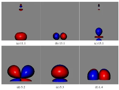
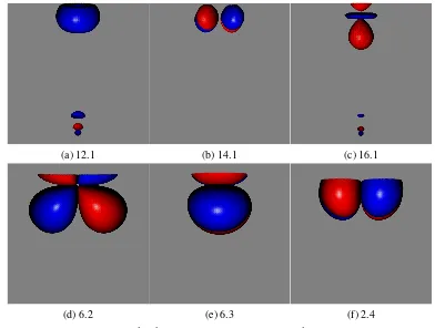
3.1 Localised orbitals for active space A in the S=1 state of Cr₂ . . . 51

3.2 Localised orbitals for active space B in the S=1 state of Cr₂ . . . 52

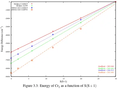
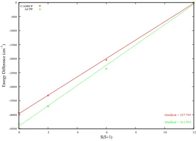
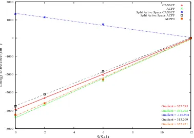
3.3 Energy of Cr₂as a function of S(S+1) . . . 57

3.4 Energy of Cr₂as a function of S(S+1)using both split and regular active spaces . . . 66

4.1 Localised orbitals for active space A in the S=1 state of N₂ . . . 75

4.2 Localised orbitals for active space B in the S=1 state of N₂ . . . 76

4.3 Baseline energies of N₂as a function of S(S+1) . . . 86

4.4 Energy of N₂as a function of S(S+1)using both split and regular active spaces . . . 91

4.5 Plot of CASSCF energies of N₂as a function of S(S+1)using the isolated orbital method . . . 95

4.6 Plot of ACPF energies of N₂ as a function of S(S+1)using the isolated orbital method . . . 95

4.7 Plot of CASSCF energies of N₂ as a function of S(S+1) using a cross atom active space . . . 102

4.8 Plot of ACPF energies of N₂as a function of S(S+1)using a cross atom active space . . . 103

5.1 Graphical representations of the two test systems . . . 114

5.2 Relative energies (eV) for the Fe(III) analogue of system A . . . 129

5.3 Relative energies (eV) for the Co(III) analogue of system A . . . 130

5.4 Relative energies (eV) for the Ni(III) analogue of system A . . . 131

5.5 Relative energies (eV) for the Fe(III) analogue of system B . . . 132

5.6 Relative energies (eV) for the Co(III) analogue of system B . . . 133

5.7 Relative energies (eV) for the Ni(III) analogue of system B . . . 134

5.8 Plots of OLYP generated Ni(III) primarily 3dbased molecular orbitals . . 138

5.9 Plots of CASSCF(ext) generated Ni(III) primarily 3dbased molecular or-bitals for system A . . . 139

6.1 Graphical representations of the two high symmetry forms of [CrII(CN)₅]3–143 6.2 Plots of the optimised geometries for the lowest energy S=2 states in-cluding the transition state. . . 147

6.3 Proposed pseudorotation mechanism for [CrII(CN)₅]3– . . . 154

6.4 Energy diagram for [CrII(CN)₅]3–pseudorotation . . . 155

7.1 Representation of the valence orbitals of the N₂molecule . . . 159

(6)

List of Tables

3.1 Molpro and MOLCAS state energies for Cr₂at 4.4 a0in D2h Symmetry . 55

3.2 State energies for Cr₂ at 4.4 a0 in C2v Symmetry using localised orbitals

and split active spaces . . . 56 3.3 Molpro and MOLCAS Cr₂state energies (cm−1) relative to the S=5 state. 58 3.4 Molpro and MOLCAS J values for Cr₂ compared to appropriate paper

values . . . 59 3.5 Comparison of D2hand C2vCASSCF state energies for Cr2 . . . 60

3.6 Comparison CASSCF state energies for Cr₂ using delocalised and lo-calised orbitals . . . 62 3.7 Comparison of CASSCF state energies for Cr₂ taking into account all

changes . . . 63 3.8 Comparison of ACPF state energies for Cr₂taking into account all changes 64 3.9 J values for Cr₂compared to appropriate Molpro results from chapter 3 . 65 3.10 Regular and split active space Cr₂ state energies (cm−1) relative to the

S=5 state. . . 67 4.1 The restricted spaces A,B,C and D for each investigated orbital pair . . . 79 4.2 The restricted spaces A,B and C for each investigated orbital pair . . . 81 4.3 Regular and split active space calculations on N₂state energies (Eh) . . . 83

4.4 State energies (Eh) for CASSCF and ACPF calculations using isolated

orbitals . . . 84 4.5 State energies (Eh) for CASSCF and ACPF calculations using cross atom

restricted active spaces . . . 85 4.6 Baseline N₂state energies (cm−1) relative to the S=3 state. . . 87 4.7 Comparison CASSCF state energies for N₂ using delocalised and

lo-calised orbitals . . . 89 4.8 Comparison ACPF state energies for N₂ using delocalised and localised

orbitals . . . 90 4.9 Regular and split active space N₂ state energies (cm−1) relative to the

S=3 state. . . 92 4.10 J values for N₂using Molpro ACPF and CASSCF . . . 93 4.11 ACPF and CASSCF N₂ state energies (cm−1) relative to the S=3 state

for isolated orbital calculations. . . 94 4.12 J values for N₂using the isolated orbital method . . . 96 4.13 Eigenvalues of the local orbitals in the S=1 state of N₂. . . 97 4.14 Comparison of baseline split ACPF and 3.1/4.1 orbital isolated ACPF

(7)

4.16 ACPF and CASSCF N₂ state energies (cm−1) relative to the S=3 state

using a cross atom active space . . . 101

4.17 Comparison of baseline split CASSCF and 1.2/2.2 orbital cross atom ac-tive space energies . . . 105

4.18 Comparison of baseline split CASSCF and 3.1/4.1 orbital cross atom ac-tive space energies . . . 106

4.19 Comparison of baseline split ACPF and 3.1/4.1 orbital cross atom active space energies . . . 107

4.20 Comparison of baseline split ACPF and 5.1/6.1 orbital cross atom active space energies . . . 108

5.1 Initial coordinate set for system A . . . 116

5.2 Initial coordinate set for system B . . . 117

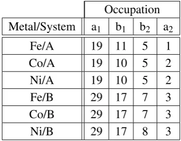
5.3 Orbital occupations for System A . . . 118

5.4 Orbital occupations for System B . . . 118

5.5 Occupation numbers used in MOLCAS HF-SCF calculations . . . 120

5.6 Occupation numbers used in Molpro CCSD(T) calculations on system A . 122 5.7 Occupation numbers used in Molpro CCSD(T) calculations on system B . 122 5.8 Raw data from DFT, CASSCF, CASPT2 and CCSD(T) calculations on system A . . . 124

5.9 Raw data from DFT, CASSCF, CASPT2 and CCSD(T) calculations on system B . . . 125

5.10 Relative energies for system A including OLYP data. . . 127

5.11 Relative energies for system B including OLYP data. . . 128

6.1 Initial coordinate set for trigonal bipyramid . . . 144

6.2 Initial coordinate set for square base pyramid . . . 144

6.3 Orbital occupations for geometry optimisations of [CrII(CN)₅]3– . . . 145

6.4 Initial coordinate set for transition state . . . 146

6.5 Occupation numbers used in MOLCAS HF-SCF calculations . . . 150

6.6 Raw data from DFT, CASSCF, CASPT2 and CCSD(T) calculations on [CrII(CN)₅]3– . . . 151

6.7 energies relative to5a1state of the trigonal bipyramid for calculations on [CrII(CN)₅]3– . . . 153

7.1 Optimised geometry of [FeIIICl(CH(CHO)₂)₂] . . . 171

7.2 Test active space configurations for [FeIIICl(CH(CHO)₂)₂] . . . 172

7.3 constructed orbital set for [FeIIICl(CH(CHO)₂)₂] listed by file and orbital use. . . 175

7.4 Raw data from calculations on [FeIIICl(CH(CHO)₂)₂]. . . 176

7.5 Dominant orbital configuration in the CASSCF for all tests . . . 176

7.6 Optimised geometry of [CrVN(CH(CHO)₂)₂] . . . 179

7.7 constructed orbital set for [CrVN(CH(CHO)₂)₂] listed by file and orbital use. . . 180

7.8 Raw data from S= 1₂ and S= 5₂ a1 constructed orbitals set calculations on [CrVN(CH(CHO)₂)₂]. . . 182

7.9 Dominant orbital configuration in the CASSCF for all tests . . . 182

(8)

A.2 Cartesian coordinates for system A Fe(III)2A2. . . 187

A.3 Cartesian coordinates for system A Fe(III)4B1. . . 188

A.4 Cartesian coordinates for system A Fe(III)4B2. . . 188

A.5 Cartesian coordinates for system A Fe(III)6A1. . . 189

A.6 Cartesian coordinates for system B Fe(III)2A1. . . 190

A.8 Cartesian coordinates for system B Fe(III)4B1. . . 192

A.9 Cartesian coordinates for system B Fe(III)4B2. . . 193

A.11 Cartesian coordinates for system A Co(III)1A1. . . 195

A.12 Cartesian coordinates for system A Co(III)3B1. . . 196

A.13 Cartesian coordinates for system A Co(III)3B2. . . 196

A.16 Cartesian coordinates for system B Co(III)1A1. . . 198

A.17 Cartesian coordinates for system B Co(III)3B1. . . 199

A.18 Cartesian coordinates for system B Co(III)3B2. . . 200

A.21 Cartesian coordinates for system A Ni(III)2B1. . . 203

A.23 Cartesian coordinates for system A Ni(III)4A1. . . 204

A.25 Cartesian coordinates for system A Ni(III)4A2. . . 205

A.26 Cartesian coordinates for system B Ni(III)2B1. . . 206

A.28 Cartesian coordinates for system B Ni(III)4A1. . . 208

A.30 Cartesian coordinates for system B Ni(III)4A2. . . 210

B.1 Cartesian coordinates for [CrII(CN)₅]3– trigonal bipyramid1A1(A). . . . 211

B.2 Cartesian coordinates for [CrII(CN)₅]3– trigonal bipyramid1A1(B). . . . 212

B.3 Cartesian coordinates for [CrII(CN)₅]3– trigonal bipyramid1A1(C). . . . 212

B.4 Cartesian coordinates for [CrII(CN)₅]3– trigonal bipyramid3B1(A). . . . 213

B.5 Cartesian coordinates for [CrII(CN)₅]3– trigonal bipyramid3B1(B). . . . 213

B.6 Cartesian coordinates for [CrII(CN)₅]3– trigonal bipyramid3B2(A). . . . 214

B.7 Cartesian coordinates for [CrII(CN)₅]3– trigonal bipyramid3B2(B). . . . 214

B.8 Cartesian coordinates for [CrII(CN)₅]3– trigonal bipyramid5A1. . . 215

B.9 Cartesian coordinates for [CrII(CN)₅]3– square based pyramid1A1(A). . . 216

B.10 Cartesian coordinates for [CrII(CN)₅]3– square based pyramid1A1. (B) . . 216

B.11 Cartesian coordinates for [CrII(CN)₅]3– square based pyramid1A1. (C) . . 217

B.12 Cartesian coordinates for [CrII(CN)₅]3– square pyramid3A1. . . 217

(9)

Acknowledgements

Over my years at The University of Warwick I have met many people without whose help and support I would not have reached this far.

First of all, I would like to thank my supervisor Professor Peter Taylor whose help and support has been instrumental in producing this thesis. Without his guidance and sparks of genius none of this would have been possible.

During my PhD I have meet many wonderful people who both as friends and col-leagues have provided much needed support and guidance whenever it has been needed. For this I would like to thank Dr. Guilherme Arantes, Devan Bailey, Jay Bomphrey, Dr. James Burnside, Dr. Christian Diedrich, Dr. Natalie Gilka, Dr. Remco Havenith, Dr. Rob Hawtin, Dr. David Quigley, Dr. Adam Skelton, Dr. Espen Tangen. A special thank you goes to Dr. Kaz Yousaf and Dave Haggart who have helped and supported me at every turn.

I would also like to thank members of the University of Warwick archery club and it’s associates who are too numerous to name for their friendship and support throughout my university career.

(10)

Declaration

(11)

Summary

Two new methods to aid in the calculation ofab initioenergies are presented.

The first method sets out to change the way that systems that have multiple elements that would benefit from a multireference treatment are handled. The method proposes splitting the system into multiple small active spaces in order to avoid the computational issues present with a single large active space. The method is developed using localised orbitals and tested on Cr₂and the molecule N₂both at long bond lengths.

(12)

List of Abbreviations

ACPF Averaged coupled-pair functional ANO Atomic natural orbital

AO Atomic orbital

AUG-CC Augmented correlation consistent B3 Becke three parameter exchange functional BSSE Basis set superposition error

CASPT2 Second order multireference perturbation theory CAS Complete active space

CCSD(T) Coupled cluster with single and doubles and pseudo-triples CC Correlation consistent

CGTO Contracted Gaussian type orbital CI Configuration Interaction

CSF Configuration State function DFT Density functional theory GTO Gaussian type orbital HF Hartree-Fock

HOMO-x The orbital x below the HOMO HOMO Highest occupied molecular orbital IVO Improved virtual orbitals

(13)

MO Molecular orbital

MPx The x-th order Møller-Plesset Perturbation Theory Me The methyl functional group

O OPTX exchange functional

PBE Perdew, Berke and Ernzerhof correlation functional PGTO Primitive Gaussian type orbital

PVDZ Valence double-zeta with polarisation Ph The phenyl functional group

RAS Restricted active space RHF Restricted Hartree-Fock SCF Self consistent field STO Slater-type orbital

SVP Split valence plus polarisation

TZVP Triple-zeta valence plus polarisation

(14)

Chapter 1 Introduction

1.1 Background

“It is unworthy of excellent men to lose hours like slaves in the labor of calculation which could be relegated to anyone else if machines were used.”

Gottfried Wilhelm von Leibniz

(15)

com-bined a calculation can quickly expand to a size where multireference methods are no longer feasible.

1.2 Aims

The aim of this thesis was to find new and inventive procedures to aid in the calculation of the type of large transition metal systems so popular at the moment. These systems have many important uses from solar power [1] to models of enzyme behaviour [2]. These systems are normally too large or complex for the kind of accurate post Hartree-Fock methods that produce the best results.

In order to meet this aim two methods have been presented which tackle the main problems preventing the use of these methods for large transition metal systems. These problems include the presence of multiple metal centres and the complexity of the orbital interactions around those metal centres.

1.3 Overview

This thesis can be split into three sections, one for each of the proposed methods and a third containing investigations into two interesting systems discovered during the course of this thesis. A short summary of each section is detailed below.

A method for the calculation of multi-metal centre containing compounds using a number of small localised active spaces is proposed and investigated in chapters 3 and 4. Chapter 3 introduces the methods and initial test system used in this investigation the Cr₂dimer. Chapter 4 investigates in detail a a second test system the N₂ molecule. This chapter also presents some extensions of the method.

(16)

practical examples of the method in use on transition metal centred complexes.

An investigation into the use of a an interesting DFT functional and its applications are covered in chapter 5. Here DFT/B3-LYP, CASSCF, CASPT2 and CCSD(T) calcu-lations are used to assess the validity of information produced about complexes of the form (nacnac)MIII(NPh) using OLYP, a functional constructed with the OPTX exchange functional and the LYP correlation functional.

(17)

Chapter 2 Theory

2.1 References

A number of books and sets of lecture notes were used in the production of this thesis and particularly in this chapter. Rather than quote each part used, the references for the entire books and sets of notes are presented here.

The books used were Introduction to Computational Chemistry [3] and the European Summerschool in Quantum Chemistry 2005 books [4, 5, 6]. Also lecture notes by Prof. Peter Taylor, and notes by Prof. Jeremy Harvey were used [7].

2.2 Introduction

Chemistry is the study of how atoms interact with each other. In the world of Experi-mental Chemistry this is usually done through the mixing and reacting of various chem-ical compounds (collections of atoms formed in to complex molecules) to form new and novel compounds. In the world of Computational and Theoretical Chemistry, however, the study of these interactions is done at a more fundamental level.

In Theoretical and Computational Chemistry, mathematical equations are used to characterise the interactions that, when put together, describe how atoms interact to form molecules, and how these molecules react to, and with, each other.

(18)

particles that make up the atoms. These particles can be split in to two groups: the nucleus, consisting of protons and neutrons, and the electrons that surround the nucleus.

There are two ways of looking at the interactions between particles in a system. The classical Newtonian method which works well for heavy slow moving objects such as buildings and people, and quantum mechanics which works better when the objects of interest are extremely light and small.

An atom, in general, is on the borderline between the classical and quantum mechan-ical regimes. Atoms moving with respect to one another can be described within both regimes, but if the interaction between the nucleus and electrons, or between a number of individual electrons is needed, a quantum mechanical method is required.

This thesis will concentrate on the interactions between electrons within atoms and molecules as they relate to chemical bonds and and other properties of these systems. As such this section will be limited to the use of quantum mechanics as a method for understanding these interactions.

2.2.1 Atomic Units

In order to simplify the representations of the various equations in this thesis the system of units used is atomic units (au). This system of units simplifies the equations by setting various important physical quantities involved in electronic structure and quantum me-chanics to one. The quantities involved are the mass of an electron (me), (e) represents minus the charge on an electron, the Bohr radius (a0) and the reduced Plank’s constant

(¯h). This incidentally leads to a new unit for energy in an atomic system called the Hartree (EH) which is equal to 4.360×10−18J.

2.3 The Schr¨odinger Equation

(19)

system as a whole can be described.

The basic equation used for quantum mechanics at a molecular level is the time-independent Schr¨odinger, equation which can be represented as shown in equation (2.1),

H(τ1,τ2. . .τN)Ψ(τ1,τ2. . .τN) =EΨ(τ1,τ2. . .τN) (2.1)

In equation (2.1)His the Hamiltonian operator,Ψis the wave function of the system, Eis total energy of the system andτithe co-ordinates of theithparticle in the system. The Hamiltonian operator is the sum of the kinetic energy (T) and potential energy (V). The wave functionΨcontains all the information about the system.

This equation can be solved exactly, but only for systems with up to two bodies such as in the Hydrogen atom which consists of one proton in the nucleus and one electron surrounding it. For larger systems such as the helium atom or any molecule, the equation has a larger number of variables. There is no way of solving the set of equations generated by such a system for all variables analytically. As such the use of the full time-independent Schr¨odinger equation is not possible for the study of the type of systems of interest to today’s Chemists.

In order to make the time-independent Schr¨odinger equation useful to Chemists, sim-plifications of the equation are needed to allow a solution for a many body system. The simplified equation must be able to accurately predict the properties of systems compris-ing many atoms.

The first thing to consider when looking at ways to simplify the

tiindependent Schr¨odinger equation is what parts of the system require quantum me-chanical treatment. In an atom, most of the mass is in the nucleus (in the form of protons and neutrons). Comparing a proton and an electron, the proton is approximately two thousand times more massive than the electron. From this comparison an assertion can be made that the electrons, being much lighter, are also moving at a much higher speed and are therefore the parts of the system most requiring quantum mechanical treatment.

(20)

(fast). This approximation allows the separation of the electronic and nuclear parts of the time-independent Schr¨odinger equation.

The Born-Oppenheimer approximation gives rise to a new form of the

Schrödinger equation as a separate electronic Schrödinger equation, as shown in (2.2), and a nuclear Schrödinger equation.

H(ri;RA)Ψ(ri;RA) =E(RA)Ψ(ri;RA) (2.2)

In equation (2.2) i runs over the electrons in the system and A runs over the nu-clei. This gives Ψ(ri;RA) as a set of different electronic wave functions over RA the co-ordinates of fixed nuclei. E(RA), then defines the potential energy surface for nuclear motion, andH(ri;RA)is the Hamiltonian operator.

For the electronic Schr¨odinger equation the form of the Hamiltonian operatorH(ri;RA) can be seen in (2.3).

H=−

∑

i 1 2∇

2

i −

∑

A

∑

i

ZA rAi

+

∑

i>j 1 ri j

+

∑

A>B ZAZB

RAB

(2.3)

In equation (2.3) ∇2_i is defined as in (2.4), Za is the charge on nucleus A, rAi is the distance between nucleus A and electron i, ri j is the distance between electron i and electron j andRAB is the distance between nucleus A and nucleus B.

∇2

i =

(

∂2

∂X_i2+

∂2

∂Y_i2+

∂2

∂Z_i2

)

(2.4)

2.4 Hartree-Fock

(21)

systems of electrons orbiting a central nucleus, in set orbitals each holding up to two spin paired ( i.e. one electron spin up (α) and one electron spin down (β)) electrons. From this model a wave function can be constructed by allocating electrons pair-wise, to molecular orbitalsψ. These molecular orbitals can then be modelled by Slater determinants which are the antisymmetrised orbital products.

The first step in forming the Hartree-Fock equations is to look at the problem at a very basic level. The electronic Schr¨odinger equation can be solved for the case of the Hydrogen atom. This solution can also be shown for other one electron systems such as He+ as the electronic Schr¨odinger equation has no reliance on the mass of the nucleus, only on its position. In order to move beyond a one-electron problem the interaction between electrons must be considered. The obvious place to start is to consider a case of non-interacting electrons. For this a model system of H−is used. If the electrons are non-interacting, the Hamiltonian could be separated into a sum of one electron Hamiltonians. The separation of the Hamiltonian results in a separation of the total electronic wave functionΨ(r1,r2) into a a number of atomic wave function. The separation of the total

electronic wave function for H− would result in two atomic Hydrogen wave functions as shown in equation (2.5).

Ψ(r1,r2) =ΨH(r1)ΨH(r2) (2.5)

The assumption of non-interacting electrons is a large one, but it is a starting point for an approach to multi-electron systems. This approach can be extended to the general form as shown in equation (2.6) which is known as the Hartree Product.

ΨHP(r1,r2, . . . ,rN) =ϕ1(r1)ϕ2(r2). . .ϕN(rN) (2.6)

In equation (2.6)ΨHPis the Hartree product wave function andϕN(rN)represents the Nthspatial orbital.

(22)

indistinguishable from one another.

Consider a two electron wave function (2.7) formed using a Hartree product as de-scribed in equation (2.6).

Ψ(r1,r2) =ϕ1(r1)ϕ2(r2) (2.7)

The wave function (2.7) produced is not a valid expression as it does not give the same product as the equally valid wave function (2.8) below.

Ψ(r2,r1) =ϕ1(r2)ϕ2(r1) (2.8)

The solution to the problem of indistinguishable electrons is to take a linear combi-nation of the Hartree products with the the electrons in different positions. For the two electron system used previously this produces two solutions as shown in equations (2.9).

Ψ(r1,r2) =

    

ϕ1(r1)ϕ2(r2) +ϕ1(r2)ϕ2(r1)

ϕ1(r1)ϕ2(r2)−ϕ1(r2)ϕ2(r1)

(2.9)

Either of these wave functions are, in principle, a valid solution to the system how-ever, experimental observation has shown that in electron containing systems, the wave function changes sign on exchange of electrons. This is the heart of the Pauli Principle. The Pauli principle states that “Valid electronic wave functions must change sign upon exchanging the co-ordinates of any two electrons”.

Of the two linear combinations, only the second of the two forms shown in (2.9) has this property.

(23)

Ψ(He) =ϕ1s(r1)ϕ1s(r2)−ϕ1s(r2)ϕ1s(r1)

=0 (2.10)

Obviously this result which suggests that helium would not form, is not correct as helium is a well documented element. There is obviously still a flaw in the construction of the wave function. The current model used to represent an atomic or molecular system takes in to account only the the electronic properties of the electrons and their position in space. There is another property of electrons that can be used to distinguish one electron from another, this property is called spin. Spin is an intrinsic property of electrons related to how they interact with a magnetic field. Electrons have two possible spin states, here represented asα andβwhich are equivalent to a positive one half spin or a negative one half spin respectively.

When creating orbital representations of a system it is possible to put two electrons in a single orbital only if the two electrons have opposite spins. This property must therefore be represented in the wave function to get a non-zero product in doubly occupied orbitals. In order to represent spin in a wave function a new co-ordinate must be introduced, this fourth co-ordinate isωor the spin “co-ordinate” . From this new model a one electron wave function is represented as follows in equation (2.11).

χ(e−) =χ(xe−,ye−,ze−,ωe−)

=χ(r,ω)

=χ(X) (2.11)

In equation (2.11) χ(X)is a spin orbital which can be derived from a spatial orbital

(24)

χ(X) =                 

ϕ(r)×α(ω) =ϕ(r)α=ϕ(r)

Or

ϕ(r)×β(ω) =ϕ(r)β=ϕ(r)

(2.12)

The use of spin orbitals (χ(X)) provides a way to write the helium wave function in a way that produces a non-zero sum as shown in equation (2.13).

Ψ(He)(x1,x2) =χ1(x1)χ2(x2)−χ1(x2)χ2(x1)

Where       

χ1 =ϕ1s(r)α

χ2 =ϕ1s(r)β

(2.13)

Writing wave functions as the antisymmetrised products of spin orbitals soon becomes tedious as the size of the system increases, therefore a simpler general representation is required, this comes in the form of Slater determinants as shown for the general case below in (2.14).

Ψ(x1,x2,x3, . . .xn) = 1

√

nelec!

χ1(x1) χ2(x1) χ3(x1) ··· χn(x1)

χ1(x2) χ2(x2) χ3(x2) ··· χn(x2)

χ1(x3) χ2(x3) χ3(x3) ··· χn(x3)

..

. ... ... . .. ...

χ1(xn) χ2(xn) χ3(xn) ··· χn(xn)

(2.14)

These Slater determinants are still time consuming to write, a simpler way of repre-senting them is shown in (2.15) where Bra-ket notation is used.

(25)

With the various methods above it is now possible to write an approximate molecular wave function in terms of Slater determinants (ΨSD) as shown below in equation (2.16).

ΨSD(x1,x2, . . .xn) =

A

{

nelec

∏

i=1

χ1(xi)

}

where: χi(xi) =ψi(ri)αorψi(ri)β (2.16)

here

A

is the antisymmetrisation operator.

The unknown molecular orbitalΨi(ri)is universally expanded as a set of “basis func-tions” as shown in (2.17). For further information on these “basis funcfunc-tions” see sec-tion 2.4.1.

ψi(ri) =

nbasis

∑

j

ci jϕj(ri) (2.17)

In (2.17)ci j is the expansion coefficient for a known basis functionϕj.

The next step is to find the values of the coefficients ci j, this is achieved by approx-imating a solution to the electronic Schr¨odinger equation. In order to find the best ap-proximate solution the variational principle is used. The variational principle states that any approximate wave function will produce a higher energy solution than the exact wave function would. Therefore the approximate wave function that produces the lowest energy solution will give the best description of the exact wave function.

In order to use the variational principle an energy must be calculated from the elec-tronic Schr¨odinger equation. The equations below show how the energy of an approxi-mate wave function can be calculated in longhand or using a normalised wave function in Bra-ket notation (2.18).

E=                    ∫

Ψ_∫(x)HˆelecΨ(x)dx

Ψ(x)Ψ(x)dx

Or

⟨Ψ|H|Ψ⟩

⟨Ψ|Ψ⟩

(26)

In order to calculate an energy for a Slater determinant wave function (ΨSD) the math-ematical expression is substituted in to (2.18) as shown below in (2.19). In order for this transformation to work the wave function must be normalised. The normalisation of the wave function when Slater determinants are used is achieved by constraining the orbitals such that they are orthonormal.

E =

∫

ΨSDHˆelecΨSDdx (2.19)

In equation (2.19)ΨSDis as shown in (2.14) and ˆHeleccan be represented as shown in (2.20).

ˆ Helec=

N

∑

A N

∑

B>A ZAZB

RAB

+

n

∑

i=1

ˆ hi+

n

∑

i n

∑

j>i 1 ri j

(2.20)

In (2.21) the Hamiltonian operator has been split into three parts the first part of the sum does not depend on electron co-ordinates, the second part is a sum of one electron operators (ˆhi) of a form shown in (2.21) and the final part is a sum of two electron contri-butions.

ˆ

hi=−∇

2 i 2 − N

∑

A

+ZA

riA

(2.21)

The result of the expanding (2.19) using ˆHelecfrom (2.20) is shown in (2.22) below.

ESD= ∫ Ψ { N

∑

A N

∑

B>A ZAZB

RAB } Ψdx + ∫ Ψ { n

∑

i=1

ˆ hi } Ψdx + ∫ Ψ { n

∑

i n

∑

j>i 1 ri j

}

Ψdx

(2.22)

(27)

energy of inter-nuclear coulombic repulsion. ∫ Ψ { N

∑

A N

∑

B>A ZAZB

RAB

}

Ψdx=

N

∑

A N

∑

B>A ZAZB

RAB

=VNN (2.23)

The other two terms can be re-written as sums of integrals (2.24).

ESD=VNN+ n

∑

i=1 {_∫

Ψ_hˆ_i_Ψ_dx

} + n

∑

i n

∑

j>i {_∫ Ψ 1

ri jΨ dx

}

(2.24)

The first sum represents the one-electron interactions. These can be simplified to Te,i the electronic kinetic energy andVNe the potential energy due to nuclear-electronic coulombic attraction, via the one-electron energies of an orbitalhiias shown in (2.25) and (2.26) whereiis an electron in the orbital.

n

∑

i=1

hii= n

∑

i=1 {_∫

Ψ_hˆ_i_Ψ_dx

}

=

n

∑

i=1 {_∫

χihˆiχidxdω

}

(2.25)

hii= ∫

χi

(

−∇2i

2 − N

∑

A ZA riA )

χidrdω

=− ∫ χi ( ∇2 i 2 )

χidrdω−

∫ χi ( N

∑

A ZA riA )

χidrdω

=Te,i+VNe,i (2.26)

The final sum represents the two electron interactions calledVee: the potential energy due to electron-electron coulombic repulsion.

(28)

∫∫

χi(x1)χj(x2)

1 r12χi

(x1)χj(x2)dx1dx2

−∫∫ χi(x1)χj(x2)

1 r12χi

(x2)χj(x1)dx1dx2

−∫∫ χi(x2)χj(x1)

1 r12χ

i(x1)χj(x2)dx1dx2

+

∫∫

χi(x2)χj(x1)

1 r12χ

i(x2)χj(x1)dx1dx2 (2.27)

In (2.27) the first and last term and the second and third term are identical pairs. These pairs of identical terms represent the two main two electron interactions.

The first pair formJi j the coulomb integral (which represents the coulombic interac-tion between electrons) and is shown in terms of real spatial orbitals and co-ordinates in (2.28)

Ji j= ∫∫

ψ2

i(r1)

1 r12ψ

2

j(r2)dr1dr2 (2.28)

The second pair formKi j the exchange integral (which represents a quantum mechan-ical effect related to the exchange of electrons in a wave function) and is shown in terms of real spatial orbitals and co-ordinates in (2.29)

Ki j = ∫∫

ψi(r1)ψj(r2)

1 r12ψ

i(r2)ψj(r1)dr1dr2 (2.29)

These integrals are related toVeeas shown in (2.30).

Vee=Jee−Kee= nelec

∑

i nelec

∑

j>i

(Ji j−Ki j) (2.30)

The result of the simplified energy equation is shown below in (2.31).

(29)

2.4.1 The Self-Consistent Field (SCF) Method

There is now a set of equations that describe the relationship between the Slater determi-nant wave function and the energy, which means the orbital coefficients ci j (as defined in (2.17)) can be found. However some of the terms in the energy expression such as the two electron terms, are dependent on the form of the orbitals. This creates a situation where an exact value for the energy is needed to calculate the orbital coefficients, and an exact description of the orbital coefficients is required to calculate the energy. There is a method for solving this kind of contradiction, this method is the Self-Consistent Field (SCF) method, which takes an iterative approach to a solution. The general procedure for the SCF method for solving this system is:

1. Guess a set of orbital coefficients

2. Construct a set of orbitals

3. Calculate new orbital coefficients (by minimising the energy)

4. Compare to previous set of coefficients. If the two sets match to a given threshold stop or else repeat from 2 with new orbitals.

Now a method is required to minimise the energy with respect to the orbitals. This takes the form of a set of simultaneous equations with the orbital coefficients as the variables. This set of equations is usually expressed as a matrix equation shown below for the closed shell case in (2.32) where the variables are collected into matrices.

∑

j

Fi jCjx=

∑

j

Si jCjxεx

where

Fi j =hi j+

∑

mn

Dmn

[

(i j|mn)−1

4(im|jn)− 1

4(in|jm)

(30)

and

Dmn=2 occ

∑

x

CmxCnx (2.32)

In (2.32)Fis the Fock matrix,Sis the overlap matrix,Dis the density matrix andCjx

is the matrix of orbital coefficients. The indicesi jrepresent occupied orbitals whilstmn represent the unoccupied orbitals.

This matrix equation produces a new set of orbital coefficients which can then be used in the SCF procedure.

In order to form the Fock matrix (F) integrals over the one and two electron operators in the Hamiltonian must be calculated. In order to calculate the Fock matrix bothhi j and

(i j|mn)must be calculated. hi j is part of the one electron operators as shown in (2.33)

hi j = ∫

ψi(r1)

(

−1

2∇

2₋

∑

A

ZAr_A−₁1

)

ψj(r1)dr1 (2.33)

and(i j|mn)is part of the two electron operators as shown in (2.34).

(i j|mn) =

∫∫

ψi(r1)ψj(r1)

1 r12ψm

(r2)ψn(r2)dr1dr2

=

∫∫

ψi(r1)ψm(r2)

1 r12ψj

(r1)ψn(r2)dr1dr2 (from (2.27)) (2.34)

(31)

produce the desired orbitals, and much easier to calculate integrals over. These so called Gaussian type orbitals use one or more Gaussian functions of the form shown in (2.35). In practise in many techniques higher angular momenta orbitals are expressed as true spher-ical harmonic Gaussians. The true spherspher-ical harmonic Gaussians produce an equal or smaller number of basis functions at higher angular momenta and thus reduce calculation times [8].

X_AlY_AmZ_Ane−αrA2 _(2.35)

In early calculations a single basis function (set of Gaussian functions) was used to represent each atomic orbital occupied in a molecular orbital. This minimal, or single-zeta (SZ), basis is too small and inflexible to describe how the atomic orbitals deform in a molecular orbital and so give poor results. A larger basis set is required to produce a good representation of a molecular orbital. These larger basis sets are produced by increasing the number of functions of a type in the set. One way to increase the number of functions is to include more functions describing each orbital, for example two functions per orbital is a double-zeta (DZ) basis set.

There is now enough information to construct a Hartree-Fock wave function and solve the SCF equations to minimise the orbitals and get an energy. However with all the approximations the variational principle says that the energy produced by this method will always be higher than the true energy of the system. There is still a part of the system left undescribed, this part is represented by a correction to the energy called the correlation energy, and is the representation of another quantum mechanical interaction between electrons.

The correlation energy can be expressed as shown in the following equation (2.36)

Ecorr=Eexact−EHF (2.36)

(32)

In the next few sections, a variety of methods which attempt to account for this corre-lation energy will be described.

2.5 Density Functional Theory (DFT)

Density Functional Theory (DFT) attempts to provide an improvement to the representa-tion of a quantum system, when compared to methods such as Hartree-Fock. It does so by including a representation of both the exchange and correlation quantum phenomenon, whereas the Hartree-Fock method only represents exchange.

The full expression for the energy of a system can be expanded with correlation as shown below in (2.37).

Eexact =VNN+Tee+VNe+Vcoul+Vx+Vc (2.37)

Equation (2.37) is an extended version of (2.31). HereVeehas been expanded asVcoul the energy due to electron-electron coulomb interactions andVxthe energy due to electron exchange. The energy due to correlation has been added in the form ofVc.

The correlation energy describes the energy of an effect known as correlation. Cor-relation describes the fact that there is an amount of correlated interaction between elec-trons. This interaction affects the movement of these electrons relative to one another; this effect, like exchange, is a quantum effect.

In defining DFT the first thing to realise is that the exchange and correlation energy terms can be combined into a single termVxc. With a suitable functional form forVxc, the energy only depends on the electron density (D_λσ).

(33)

ψi=

∑

µ

χµCµi

D_λσ=2

∑

i

C_λ_iC_σi (2.38)

Molecular orbitals formed this way are called Kohn-Sham orbitals. These orbitals do not represent a physical property or the form of an electronic orbital of the system, rather they describe an area of electronic density. They are often used for interpretation in the same way that LCAO orbitals are in Hartree-Fock, but as they do not represent the same property this can lead to errors in interpretation.

The energy of a system can now be written as a function of the densityD_λσ as shown in (2.39) below.

EDFT[D_λσ] =VNN[D_λσ] +Tee[D_λσ] +VNe[D_λσ] +Vcoul[D_λσ] +Vxc[D_λσ] (2.39)

The functional form of each term in (2.39) is known and can be easily calculated using various methods except forVxc. There is no known exact functional form forVxcso approximations must be made. There are three main methods for defining a functional for Vxc, Local Density Approximation (LDA) [9, 10], gradient-corrected methods or hybrid

methods. All these methods with the exception of LDA involve a certain amount of fitting the parameters in the functional to a given data set. DFT sits somewhere between Ab Initiomethods, where everything can be defined from first principles, and semi-empirical methods which use empirical data to fit many of the parameters for calculation.

2.5.1 Functionals

As stated above there are three main methods for approximation of the functional forVxc each method will be detailed below.

(34)

the electron density. The critical assumption in LDA is that the local density at any point in a molecule can be satisfactorily described as a uniform electron gas, and therefore the density seen by each electron is uniform throughout the molecule. This assumption obviously does not hold up for most single molecules, as there are obvious areas of high electron density about bonds and areas of low electron density or no electron density at the nuclei. This approach might work better in extremely large and diffuse molecules where the density is more uniform, or in large systems such as metals or semi-conductors. Here the electrons form bands which have a relatively uniform density. The LDA can be expanded to include separate orbitals and densities forα andβspin electrons; in this form it is called the Local Spin Density Approximation (LSDA) [11, 10]. The LSDA has a number of advantages, the most obvious being that it allows calculations of systems in which the electrons are not spin paired, such as radicals and some ions.

Built upon the LDA or LSDA are gradient-corrected methods. These methods com-bine the electron density with a first order correction in the form of the gradient of the density. This allows for a non-uniformity of the density seen by each electron. The in-clusion of the first-order correction to the exchange term produces a better total energy, whilst the first order correction to the correlation term often results in a positive energy for correlation, counteracting the improvement in the exchange term. This simple applica-tion of the method actually produces a worse performing model than an LSDA model. To solve this the gradient is often included as a variable, and the terms are fitted to produce a better representation of the correlation energy. This approach is know as the generalised gradient approximation (GGA).

(35)

Generally, functionals are of the hybrid type and split into an exchange part and a correlation part. These parts are often developed separately and put together in a mix and match approach in order to produce a good fit for certain quantities of interest in a given system.

One of the most popular general purpose functionals, and the one used for most DFT calculations in this thesis, is B3-LYP. It is a form of hybrid functional using the Becke three term exchange Functional (B3) [12], and the Lee, Yang and Parr correlation func-tional (LYP) [13]. This funcfunc-tional combines contributions from a number of different ex-change and correlation functionals with appropriate fitting functions as shown in (2.40). The constants used are as followsa0=0.2,ax=0.72 andac=0.81.

Vxc= (1−a0)Vx(LDA) +a0Vx(HF)axVx(B88x)

+acVc(LY P88c) + (1−ac)Vc(VW N80c)

(2.40)

The B3-LYP Functional was optimised on a number of properties of first and second row atoms. However B3-LYP is also often used to calculate properties outside those it was optimised for, and for calculations on elements outside the first and second rows.

2.5.2 Performance

(36)

spin state, is less noticeable using hybrid functionals.

The next few sections will detail a number of methods that attempt to incorporate correlation using a purely Ab Initio approach rather than the semi-empirical approach used in DFT.

2.6 Single Reference Correlation

The previous section detailed the use of DFT in order to add correlation to the description of a molecular system using semi-empirical functionals. The next two sections will focus on introducing correlation using anAb Initioapproach.

The first thing to look at is what makes up correlation. Correlation can be divided into two separate effects. The first of these effects is dynamical correlation. This describes what happens to a wave function when two electrons approach each other. The other type of correlation is non-dynamical correlation, also known as static correlation. Static corre-lation is due to near degeneracy of different electron configurations in the wave function. In order to fully describe a system, both forms of correlation must be properly accounted for.

Non-dynamical correlation can be included in a system quite easily by allowing a mixing of more than one configuration in the wave function. Methods for doing this will be discussed in the next section. Dynamical correlation is very difficult to include in a system. It takes many different configurations in order to properly describe these interactions.

There are broadly three classes of method for including dynamical correlation in a wave function, all closely related in theory. These methods are perturbation theory, con-figuration interaction (CI) and coupled cluster.

(37)

Perturbation theory solves the new problem by introducing a small change or pertur-bation into the problem. In the case of correlation this is done by defining a two part Hamiltonian consisting of a reference Hamiltonian,H0, and a perturbation,H′, with the

magnitude ofλ. The relationship is shown in (2.41).

H=H0+λH′ (2.41)

The perturbed wave function is given by (2.42).

HΨ=WΨ (2.42)

As the perturbation increases to a finite value the new energy (W) and wave function also changes continuously. The new wave function and energy can be expanded in a power series in the perturbation parameterλas shown in (2.43).

W =λ0W0+λ1W1+λ2W2+λ3W3+. . .

Ψ=λ0Ψ0+λ1Ψ1+λ2Ψ2+λ3Ψ3+. . . (2.43)

Inserting the results from (2.42) and (2.43) into the Schr¨odinger equation and collect-ing terms of the same order inλgives (2.44).

H0|Ψ0⟩=W0|Ψ0⟩

(H0−W0)|Ψ1⟩= (W1−H1)|Ψ0⟩

(H0−W0)|Ψ2⟩= (W1−H1)|Ψ1⟩+W2|Ψ0⟩ (2.44)

It can be assumed that the perturbed wave functions are orthogonal to the zeroth order wave function. This orthogonality allows a normalisation of the total wave function such that⟨Ψ|Ψ0⟩=1. This normalisation is used to produce energy expressions up to second

(38)

W0=⟨Ψ0|H0|Ψ0⟩

W1=⟨Ψ0|H1|Ψ0⟩

W2=⟨Ψ0|H1|Ψ1⟩ (2.45)

The most popular form of perturbation theory is Møller-Plesset Perturbation Theory (MP) which chooses the sum over Fock operators as the zeroth-order Hamiltonian and uses the exactVee operator minus twice the⟨Vee⟩operator. There are different orders of perturbation theory based on how far along the power series the perturbation extends. The most popular form of (MP) is second order Møller-Plesset (MP) Perturbation theory (MP2) as it is computationally cheap, although not as cheap as DFT, and seldom gives a more accurate result as it often overshoots the correlation energy.

The second method is Configuration Interaction (CI) which is similar to mixing mil-lions of different configurations. In CI the wave function is built from a linear combination of Configuration State functions (CSF). These CSF’s are constructed using a ground state Hartree-Fock determinant expanded with a number of excited state determinants.

A CI method is generally limited by the number of additional determinants used in the construction of the CSF’s. For example if any occupied orbital is replaced by a virtual orbital this is a single excitation, two is a double excitation and so on. CI methods are usually limited by the number of excitations allowed. Just single excitations are no use as all matrix elements between the single excitations and the Hartree-Fock determinants are all zero. but CID (just double excitations) and CISD (singles and doubles) are popular forms.

CI is generally less widely used than both MP2 and coupled cluster methods as it is extremely expensive computationally (although no worse than coupled cluster), especially at higher excitation levels or when used on larger systems. It only produces better results than MP2 in small systems and does not scale correctly with the number of electrons.

(39)

refer-ence treatment of correlation. It is size-extensive (it scales correctly with the number of electrons) giving it the advantage over CI methods and gives a much better result than MP2. Unfortunately these advantages come at the expense of computational speed.

In the perturbation theory method outlined above all types of correction to the refer-ence wave function are added to a given order (2,3,4, etc.). The idea with coupled cluster methods is to include all corrections of a given type to infinite order. To do this an ex-citation operator Tas shown in (2.46) is used to act on a Hartree-Fock reference wave functionΦ0whereTigenerates allith excited Slater determinants. As shown in (2.47).

T=T1+T2+T3+···+TNelec (2.46)

T1Φ0=

occ

∑

i vir

∑

a t_iaΦa_i

T2Φ0=

occ

∑

i<j vir

∑

a<b

t_{i j}abΦab_{i j} (2.47)

A CI wave function can be generated by allowing Tto work on a Hartree-Fock wave function. The corresponding CC wave function is defined as the exponential of the exci-tation operator acting on the same Hartree-Fock wave function. Both are shown in (2.48).

ΨCI= (1+T)Φ0

= (1+T1+T2+T3+T4+···)Φ0

ΨCC=eTΦo

Where

eT=1+T+1

2T

2₊1

6T

3₊_{. . .}

=

∞

∑

k=0

1 K!T

k

(2.48)

(40)

all triple excitations (triples).

eT=1+T1+ (T2+

1 2T

2

1) + (T3+T2T1+

1 6T

3

1)

+ (T4+T3T1+

1 2T

2

2+

1 2T2T

2

1+

1 24T

4 1). . .

(2.49)

So far, this wave function generates an exact solution equivalent to a full CI. However, as with a full CI, this is just not possible for anything but the smallest systems and in the same way that a CI is usually truncated to only include certain excitations, the same is applied to CC methods. For example CCSD, one of the most popular CC methods, includes only contributions fromT=T1+T2.

The addition of a full treatment of triples (CCSDT) causes a lot of added computa-tional complexity to coupled cluster calculations; however for only a small amount of extra computational work over CCSD, a perturbative treatment of triples can be used. The perturbative treatment uses equations derived from MP4 and MP5, but using CCSD amplitudes (t) rather than perturbation coefficients, this gives CCSD(T).

2.7 Multiconfigurational Effects

In order to recover a large amount of the non-dynamical correlation in a system a sin-gle reference wave function is unsuitable, as it treats only one of the many possible near degenerate electron states. This may not be a problem in a ground state system of sim-ple atoms, near its equilibrium geometry. However, once the system moves away from an equilibrium geometry, or if the system includes atoms which can exhibit a number of different and low lying valence electron configurations (such as many transition metal complexes), the number and importance of near degenerate electron states and by exten-sion non-dynamical correlation becomes much more important.

(41)

φi=Ni(χiA±χiB) (2.50)

At the equilibrium geometry the ground state is dominated by the doubly occupied

φ1 orbital ((φ1)2) which is made up from the atomic orbitals χ1A and χ1B whose main contribution is the Hydrogen 1sorbital with some “small corrections”. A qualitative rep-resentation ofφ1is shown in (2.51), here the small corrections are neglected.

φ1=N1(1sA+1sB) (2.51)

In the restricted Hartree-Fock (RHF) model the wave function is formed by doubly occupyingφ1as shown in (2.52), whereΘ2,0is the singlet spin function.

Ψ1=φ1(r1)φ1(r2)Θ2,0

Where

Θ2,0=

√ 1

2(α1β2−β1α2)

(2.52)

The RHF model like all Hartree-Fock models, works well at the equilibrium bond length; however as the bond length is changed away from equilibrium, such as when measuring a potential curve, there is a problem. In the RHF wave function as described in (2.51) as the bond length changes the form of the molecular orbital does not. The problem with this becomes clear if the wave function is expanded as the product of atomic orbitals as shown in (2.53).

Ψ1=N12[1sA(r1)1sA(r2) +1sA(r1)1sB(r2) +1sB(r1)1sA(r2) +1sB(r1)1sB(r2)] (2.53)

As can be seen from (2.53) the RHF wave function at all distances has components where both electrons appear on the same nucleus. At the equilibrium geometry this is a valid contribution, but as the H2molecule disassociates these contributions would result

in ionic terms (H++H–) in the product.

(42)

are unsuitable where there are open shell products associated. A method is therefore needed to correct for these “ionic structures”. An easy solution to this problem would be to divide the wave function into an ionic and covalent part and use inter-nuclear distance to weight the contributions of each part as shown in (2.54)

ΨV B=CionΨion+CcovΨcov

Where

Ψion=Nion[1sA(r1)1sA(r2) +1sB(r1)1sB(r2)]Θ2,0

and

Ψcov=Ncov[1sA(r1)1sB(r2) +1sB(r1)1sA(r2)]Θ2,0

(2.54)

This method produces a valence bond description of the chemical bond which gives it appeal as a chemical description; however this chemical understanding comes at the cost of mathematical simplicity. The formulation in (2.54) relies on atomic orbitals which are formed from nonorthogonal basis functions which add a great deal of complexity to the mathematical treatment. The added mathematical complexity has meant that this method is not widely used in chemistry.

The main problem with the formulation in (2.54) is the nonorthogonal basis func-tions, therefore an alternative formulation is required using an orthogonal basis. Rather than thinking about the problem as a competition of ionic and covalent configurations, this method introduces the principle of an anti-bonding orbital φ2 (2.55). In a bonding

molecular orbital the components of the constituent atomic orbitals have the same phase creating a favourable environment for electrons. In an anti-bonding molecular orbital the components of the constituent atomic orbitals are out of phase creating an unfavourable environment for electrons.

φ2=N2(1sA−1sB) (2.55)

(43)

H2. The wave function is shown in (2.56) whereΨ2is the wave function using electronic

configuration (φ2). C1 and C2 are coefficients to weight the influence of the different

configurations.

ΨMC=C1Ψ1+C2Ψ2 (2.56)

The dissociation of the Hydrogen bond is a simplistic example of the power of mul-ticonfigurational methods and also does not really show its limitations. For the most part a multiconfigurational wave function can be built in a similar way to that shown for H2

but instead of using the full atomic orbital basis, more complex examples are generally constructed from an appropriate molecular orbital basis.

As the number of orbitals which are directly involved in bonding increase, it is obvious that the number of configuration state functions (CSF’s) involved will increase. This increase is very rapid. For example, without taking into account symmetry the number of configuration state functions involved in the dissociation of the bond in H2is just two,

whereas one hundred and seventy five are required to describe the dissociation of the triple bond in N2, whilst the number of orbitals involved has only increased from two (φ1 and φ1) to six (3σg, 3σu, 1πux, 1πgx, 1πuy and 1πgy). The orbitals involved directly in the multiconfigurational calculation are called the ‘active’ orbitals.

The general equation for an MCSCF wave function is shown in (2.57)

ΨMCSCF =

∑

k

ΦKAK

Where

ΦK =A

{

∏

i⊂k

ϕi

}

and

ϕi=

∑

µ

χµCµi (2.57)

(44)

are the CSF’sΦK. AKare the associated configuration mixing coefficients. Each CSF is a product of MOsϕishown expanded in an AO basischiµ.

An MCSCF calculation can be viewed as a CI calculation where as well as configu-ration mixing coefficientsAK, the orbital coefficients (Cµi themselves are optimised. This optimisation is similar to the SCF optimisation method used in Hartree-Fock. A problem with the MCSCF wave function is that it is hard to converge and often does not find a minimum. In Hartree-Fock SCF a check that the first derivatives of the energy with re-spect to the orbital coefficients is zero is usually sufficient to check convergence although does not guarantee a minimum. In order to ensure convergence to a minimum in MCSCF a further check is made. The second derivatives of the energy with respect to the orbital coefficients is calculated. If the diagonalisation of these second derivatives produces only positive eigenvalues a minimum has been found.

A number of methods have been used to optimise the MCSCF wave function some of them are discussed below.

The Optimised Valence Configuration (OVA) method was the first practical method for optimising a MCSCF wave function. The OVA used a two step process in which first the configuration mixing or CI coefficients AK are optimised by diagonalisation of the Hamiltonian followed by an update of the orbitals. The new optimised orbital coefficients were produced by a set of coupled Fock matrix diagonalisations using a generalisation of the open and closed shell SCF techniques. This technique suffered from poor convergence due to poorly selected CSF’s and the step-wise optimisation process.

(45)

multiconfigurational character themselves. The states arising from these excitations along with reference MCSCF state form the super-CI. At convergence, the Hamiltonian matrix elements between the MCSCF wave function and the SX space must vanish. This led to several optimisation techniques attempting to drive these matrix elements to zero. A more efficient method of calculating updated orbitals was also developed at the time the GBT optimisation techniques were being developed replacing natural orbitals of the MCSCF wave function with natural orbitals of the super-CI. There was a problem with early im-plementations of this method due to the large amount of elements needing calculation in a super-CI. This is due to each single excitation being a linear combination of as many CSF’s as were contained in the MCSCF wave function. This means that in order to cal-culate a single element of the Super-CI Hamiltonian a large number of smaller matrix calculations are required, this created a bottleneck in the calculation. A solution to this problem was shown by Bj¨orn Roos [14]. He presented a method for approximating the super-CI Hamiltonian. The method used Fock matrix elements to approximate some parts of the SX-SX interactions while still maintaining exact calculation of the MCSCF-SX el-ements used by GBT to track optimisation.

The most common methods currently in use for the optimisation of MCSCF calcula-tion fall into the category of second order optimisacalcula-tion. These methods use the second derivative of the energy (the Hessian) as a convergence criterion as well as the first deriva-tive (the gradient). This was achieved by applying the Newton-Raphson method to the MCSCF wave function.

The most common method for calculating a multiconfigurational wave function is the Complete Active Space SCF (CASSCF) method. This method can be seen as a gener-alisation of the Hartree-Fock method in which the restrictions in orbital occupation have been relaxed.

2.7.1 CASSCF

(46)

MOs are chosen as those critical to the system under investigation and a “full CI” of all possible configurations of electrons within that selection of MOs is created.

In order to differentiate the important MOs they are divided in three subsets:

1. Inactive orbitals

2. Active orbitals

3. Virtual orbitals

The inactive orbitals are generally those which represent the core atomic orbitals of the atoms in the molecule, and are kept doubly occupied in the calculation. The virtual orbitals are those orbitals formed from the basis set, which are not part of either the active or inactive spaces and are therefore not occupied in any CSF. The active orbitals are most often those which form the valence orbitals in atoms, the bonding, anti-bonding or non-bonding orbitals in molecules or some important subset of these orbitals. The active orbitals are used to build the CSF’s by filling them with the remaining electrons known as the active electrons. These CSF’s are then optimised as shown in (2.56) along with the molecular orbitals. The total wave function is a linear combination of all the CSF’s that fulfil a given space and spin symmetry. This tends to lead to a spectrum of occupation numbers for the active orbitals that fall between zero and two. This method is called CASSCF because all CSF’s generated by the combination of active electrons and orbitals are included in the calculation.

Alternative approaches to orbital optimisation in first row transition metal systems

warwick.ac.uk/lib-publications

Alternative Approaches to Orbital Optimisation in

First Row Transition Metal Systems

By

Matthew John Tilling

Contents

List of Figures

List of Tables

Acknowledgements

Declaration

Summary

List of Abbreviations

Chapter 1

Introduction

1.1

Background

1.2

Aims

1.3

Overview

Chapter 2

Theory

2.1

References

2.2

Introduction

2.2.1

Atomic Units

2.3

The Schr¨odinger Equation

∑

∑

∑

∑

∑

2.4

Hartree-Fock

A

∏

A

∑

∑

∑

∑

∑

∑

∑

∑

∑

∑

∑

∑

∑

∑

∑

∑

∑

∑

∑

∑

∑

∑

∑

∑

∑

∑

2.4.1

The Self-Consistent Field (SCF) Method

∑

∑

∑

∑

∑

2.5

Density Functional Theory (DFT)

∑

∑

2.5.1

Functionals