Hardware Efficient Real Time Statistical Analysis on Streaming Data

(1)

Hardware-Efficient Real-Time Statistical Analysis

on Streaming Data

Niels Sulzer

Bachelor Assignment Committee:

dr.ing. D.M. Ziener, dr.ir. A.B.J. Kokkeler, dr.ir. R.A.R. van der Zee

Computer Architecture for Embedded Systems (CAES)

Faculty of Electrical Engineering, Computer Science and Mathematics (EEMCS)

University of Twente, Enschede, the Netherlands

November 2019

Abstract—An algorithm for statistical analysis on streaming data is designed and implemented. In the context of an audio amplifier controller, the algorithm aims at providing power statistics from voltage and current streams for real-time efficiency optimisations. To reduce computational complexity of the design, downsampled approximations of the input signals are used to calculate the statistics. Several techniques are discussed to optimise the arithmetic operations of the algorithm, with focus on serial arithmetic and eliminating the need for division. A proof-of-concept is implemented in VHDL and synthesised for UMC 65nm to give an idea of the physical size such an algorithm could have.

I. INTRODUCTION

A

MPLIFIER controllers with programmable transfer can be custom configured to match any particular load, usually a speaker. Statistical analysis of the output in real time would reveal even more opportunities to improve efficiency. Real time power statistics can be used to reduce wear on the speaker and improve audio quality by detecting and correcting for compression, and to optimise power draw to improve efficiency especially for battery powered devices.

A particular amplifier controller uses loop filter slices which allow for programmable amplifier transfer. Each loop filter slice can be configured to represent current or voltage, and thus power measurements and statistical calculations would be possible. Currently, however, there is no direct way of moni-toring the output of the loop filters on this amplifier controller chip itself. When power measurements can not be done on chip, an external DSP (Digital Signal Processor) is required to sample the data streams from the amplifier controller chip and do calculations. For each audio sample at 48kHz, the loop filter outputs one frame of 512 samples. Sampling this stream with the external DSP over I2S, regardless at which sample frequency, puts an unnecessary load on the external DSP just to acquire the stream, not to mention following calculations. The proposed solution is to integrate at least parts of the calculation of statistical measures into the amplifier controller chip itself to reduce or eliminate the need for an external DSP. This statistics block, represented by the green section in Figure 1, would be an algorithm which calculates maximum, minimum, mean and mean-squared on the streaming data from each of the eight loop filter slices (red block in Figure 1) or

power data which is a combination of one voltage and one current slice. A basic overview of the statistics block is shown in Figure 2. While there is one output for each statistic per loop filter slice, where a combination of two loop filter slices is used (for power) one of two outputs would be unused. Besides defining some loose requirements, no previous work has been done on implementing this algorithm.

This report will focus on the techniques used in such an algorithm, investigating the computational complexity of each statistical calculation at the algorithm and the hardware arith-metic level. The full algorithm for all eight loop filter slices will not be implemented. Rather, a proof-of-concept will be implemented to work on two loop filter slices (one for current and one for voltage) and calculate the statistics of either the input current of voltage stream or the combined power data, resulting in one output per statistic. The proof-of-concept will be written in VHDL and synthesised for UMC 65nm to get an approximation of the physical size of the algorithm and available slack time.

First, each statistical measure will be presented in Section II. Section III presents methods for downsampling as a way to reduce the number of calculations required to calculate each statistic. In Section IV the computational complexity of the statistical measures and their downsampled approximations are investigated with respect to the hardware arithmetic that underlies the algorithm. In Section V the design choices regarding implementation of the algorithm in hardware are detailed. The implementation in VHDL and the results of synthesis are presented in Section VI. Section VII presents discussion of the results of synthesis and suggestions for further research. Finally, Section VIII concludes this report.

II. STATISTICALMEASURES

(2)

[image:2.612.47.301.54.138.2]

Fig. 1. Basic architecture of amplifier controller chip. Statistical Measurement block in green.

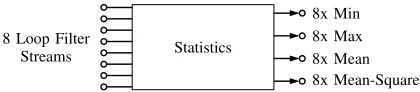
8 Loop Filter Streams

8x Min 8x Max 8x Mean 8x Mean-Square Statistics

Fig. 2. Overview of statistics block with inputs for all loop filter slices. Where a combination of two loop filter slices is used (for power) one of two outputs would be unused.

A. Mean

The meanx¯ is given by:

¯

x 1 N

N

¸

n1

xrns (1)

B. Mean-Squared

The mean-squarex¯2of a signalxrnsis a variation on RMS which does not require the computationally complex square root operation. Mean-square over N samples is defined as:

¯

x2 1 N

N

¸

n1

xrns2 (2)

C. Maximum and Minimum

The maximum (max) and minimum (min) are calculated over the same period of N samples over which mean is calculated. The difference between the maximum or minimum and the mean is a measure of the gain compression. If the audio signal is more compressed the average and maximum (or minimum) will be closer together. Determining the maximum and minimum relies on comparators comparing, bit by bit, the value of the current sample xrns to the previous sample xrn1s, and will be discussed in more detail later. What must be mentioned is the assumption that, since the signal xrns is centred around 0, the minimum and maximum will always be a negative and a positive number respectively.

III. DOWNSAMPLING

Due to the computational complexity of calculating the exact statistical measures ofN samples, some suggestions are made to reduce the number of operations required. The main method explored for reducing the number of operations is to reduce the number of samples on which the statistical measure is calculated; this is a sort of downsampling. The signal xrns, n P 1, . . . , N is downsampled by a factor w (herein also called the window size), resulting in the downsampled

approximationxˆrns, nP1, . . . ,N_w which has N_w samples. The statistical measures based on the downsampled signals are then calculated similarly to (1) and (2), but usingx. For example,ˆ

downsampled mean-squarexˆ¯2 _{would be calculated as:}

ˆ ¯

x2 1 N{w

N_¸{w

n1 ˆ

xrns2 (3)

Note that the summation is done over fewer values. For a power signal prns VrnsIrns the same principle can be applied. In this case, the methods of downsampling apply to the voltage and current signals such that the downsampled ap-proximation of prns VrnsIrns becomespˆrns IˆrnsVˆrns. For example, downsampled mean powerpˆ¯is then given by:

ˆ ¯

p 1

N{w N_¸_{w

n1 ˆ

IrnsVˆrns (4)

A. Methods for Downsampling

Two methods for downsampling are explored and compared: 1) Discarding Values: The most basic way of reducing the number of samples is taking every wth sample, discarding the rest. The downsampled approximation sequence becomes

ˆ

xrns xrnws, similarlypˆrns IrnwsVrnws[1].

2) Block Mean: A more robust method is to downsample wsamples by taking their mean. The downsampled signal of xrnsbecomes:

ˆ

xrns 1 w

kw

¸

ipk1qw 1

xris, k0, ...,N

w (5)

To approximate power using this method would require taking the mean of both the current and voltage signal to get

ˆ

IrnsandVˆrns before multiplying these, as done in (4). First multiplying Vrns and Irns and then approximating would yield no reduction in total number of operations compared to the direct method, as seen in Table I for the mean power calculation (see row: Approx. after mult.).

Block mean downsampling has more consistent perfor-mance compared to discarding values. Accuracy of the dis-carding values method suffers as quick changes in xrns are lost. Thenwth_{sample is not representative of of the past}_w₁

samples. On the other hand, discarding samples has negligible computational complexity, compared to the block mean, which requires w additions per approximated sample. Nonetheless, block mean approximation is chosen as the preferred method, as the accuracy of downsampling by discarding values is entirely up to chance.

B. External DSP

[image:2.612.69.279.182.228.2]

(3)

communication between the DSP and amplifier controller. For example, mean calculations on xrns could be split between the amplifier and the external DSP. Combining equations (1) and (5) gives:

ˆ ¯

x 1

N{w

1

w N_¸{w

k1

_kw

¸

ipk1qw 1

xris

(6)

The brackets are evaluated on the amplifier controller, and the outside is evaluated on the external DSP. The division could be moved entirely onto the DSP, since division _N1 only has to happen once. The option of offloading to the DSP is not further explored as it is not the end goal, but rather a possible intermediary solution.

IV. ARITHMETICOPERATIONS

In making the calculation of statistics a real-time process while using as few resources as possible, close attention must be paid to the computational complexity of each calculation. In order to get a sense for how computationally intensive each statistical measure and its downsampled approximation are, they are broken down into the number of basic arith-metic operations required. The basic aritharith-metic operations are addition/subtraction, multiplication (this includes squaring) and division. To add a further step of abstraction and make comparisons of computational complexity more direct, each of the arithmetic operations are reduced to the number of clock cycles required for an operation on n bits. In general, the arithmetic can be optimised for either space efficiency or speed (fewer clock cycles). Optimising for smaller area, at the expense of more clock cycles, is done by using serial arithmetic, in contrast to parallel. Each of the arithmetic operations as well as the comparator required for min and max, will be discussed with regards to the implementations that could be used in hardware. In the case of area efficiency, this mainly comes down to a choice of serial or parallel arithmetic.

A. Addition/Subtraction

[image:3.612.357.518.58.157.2]

Summation, which is central to the statistics presented, is performed using an accumulator which stores the current sum in a register then adds the next sample using one of the addition methods discussed and stores the result back in the same register [2]. The underlying operation of this operation being addition. Addition and subtraction of two’s complement numbers can be simplified by the principle aba pbq making subtraction equivalent to complementing followed by addition [3] Addition can be implemented either as a serial operation where one bit is added per clock cycle, or parallel where the entire operation occurs in one clock cycle. Serial addition takesnclock cycles per addition of twon-bit numbers [4], whereas the parallel adder takes only one. Both of these methods are useful, depending on how many clock cycles are available to compute the addition. In the downsampling block, there is only one clock cycle to compute the addition of the next sample to the sum, whereas in later blocks there are w clock cycles to add the next sample of the downsampled signal to the sum. The serial adder loads both operands into shift

Fig. 3. Finite state machine of serial adder [6]. Inputsaandbare bits from input shift registers, outputsgoes to output shift register.Y is the carry-out of the full adder.

Fig. 4. Cascade of full adders (FA) creating a parallel adder [8].

registers and a single full adder adds two bits at a time, holding the carry bit for the next set of two bits [5]. The full adder is shown in Figure 3, showing the inputs and outputs a,b, and sto and from shift registers.

The parallel adder, in contrast, requires one full adder per input bit. The carry is propagated from each adder cell to the next, owing to the name Ripple Carry Adder [4]. The cascade of 4 full adders is shown in Figure 4. An n-bit adder would require a cascade of n full adders. The downside to ripple carry adders is the long propagation delay from the first input to the last output due to the carry bit. There are methods to reduce the carry propagation delay such as carry lookahead adders [7], which will not be further discussed, but provide much opportunity for further research.

B. Multiplication

Multiplication is based on addition and shifting, and can therefore be implemented parallelly or serially. Multiplication is done by generating a partial product for each bit of the input, and then summing the partial products to get the final product [9]. The addition is done using an adder, and therefore multiplication of nbits will also take nclock cycles. Partial products are formed by combinational logic, and their addition is done in a running fashion rather than storing all partial products in the end. Parallel multiplication computes more than one partial product per clock cycle [4] in the same fashion as the serial procedure.

C. Division

[image:3.612.341.534.212.284.2]

(4)

TABLE I

COMPARISON OFCOMPUTATIONALCOMPLEXITY OFSTATISTICAL

MEASURES DIRECTLY ANDDOWNSAMPLED USINGMEAN. NUMBER OF CLOCK CYCLES CALCULATED WITHn16,N216_AND_w₁₀₂₄

Statistic Add’s Mult’s Div’s Clock Cycles

Mean Power

Exact N N 1 2097152

Downsmpl. 2N N_w 1 2098176

Downsmpl.

after mult. N N 1 2097152

Mean-Sqr. Power

Exact N 2N 1 3145728

Downsmpl. 2N 2N

w 1 2099200

V/I Mean Exact N 0 1 1048576

Downsmpl. N 0 1 1048576

V/I Mean-Square

Exact N N 1 2097152

Downsmpl. N N

w 1 1049600

free to be chosen. If the divisor is constrained to powers of two, bit shifting becomes an option. Bit shifting is the most basic method of binary division. Shifting n bits to the right is equivalent of division by 2n, hence the constraint on the divisor. When the same number format is kept after division, the downside to shifting this is the loss of precision as the rightmost n bits are lost.In an application where the number format is not fixed however, virtual shifting can be used. A virtual bit shift virtually moves the implied decimal point changing the representation of the number, but not the bit pattern [10]. This requires no shifts and results in no loss of precision, but has to be taken into account when the value is used elsewhere later.

The computational complexities of the exact and (mean) downsampled implementation of each statistical measure in terms of the basic operations are shown in Table I. The number of clock cycles required using serial addition and multiplication with n 16 bits are also given as a clear representation of the improvement in computational complex-ity from using downsampling for power and mean-square calculations. For downsampling a window size ofw1024is used. Each statistic is represented as only taking one division as all division operations could be reduced to one, however when using virtual shifting division has no computational cost anyway. Interestingly, the mean power takes more clock cycles when downsampling because of the number of additions required. On the other hand, the smaller area of an adder compared to a multiplier is not represented.

D. Comparator

As mentioned, the comparator is essential to the minimum and maximum statistics. In the same way that addition and multiplication can be run serial and parallel, so can the comparator. The serial method makes use of a combinational circuit that compares only two bits per clock cycle, and repeats this process nclock cycles to compare twon-bit words. The comparison is done MSB first. If two bits are equal, the next two bits are considered, until a difference is found [7]. The one bit comparator is based on the equations [11]:

Fig. 5. Combinational logic of 1-bit comparator [12].

(A¡B) = AB¯ (A B) =AB¯ (A=B) =A¯B + AB¯

The resulting combinational logic for a one bit comparator is shown in Figure 5. In the parallel method, a combinational more complex logic circuit takes two n-bit inputs A and B and outputs whether A=B, A¡B or A B [11]. Of course, between the fully parallel and fully serial implementations are any number of different combinations of comparing k bits at a time with combinational logic for l clock cycles where kln. In the interest of reducing the area of the circuit and considering that there arewclock cycles to complete the comparison wherew"n, a serial implementation is preferred. In the serial case where the new number, call it A, is compared to both the maximum and minimum this is done one after the other. First, A is compared to the current stored maximum Bmax. Then if A Bmax, A is compared to the current stored

minimum Bmin. This would take a maximum of 2n clock

cycles if the maximum and minimum only differ by the least significant bit and A=Bmin.

E. Number Formats

The inputs V and I (the direct output of the loop filters) are 16-bit signed (two’s complement) fixed point format with 1 integer bit and 14 fractional bits; call this format A(1,14). The range of these is from p21q to 21214 [10]. The number formats that will be used in the arithmetic are of great importance as these define the required size of arithmetic blocks and the number of clock cycles that operations take. There are two extremes to choosing number formats; maximal precision or smallest arithmetic implementation. The higher the precision, the more bits are required requiring larger hardware. The proof-of-concept will be implemented in the worst-case with respect to size, where no precision is lost throughout. This is means that any modifications made in the future should not result in a larger physical area. While the algorithm should work for anywandF, these do play a role in determining the number formats of the accumulators used in every block. For an accumulator of sizeαwith input number format A(a,b) the maximum absolute input to the accumulator will be |p2aq|, and the maximum number reached by the accumulator will therefore beα2a, requiringlog2α a bits.

(5)

F. Window Size

Until this point, the downsampling window size has al-ways been left as w, and the total samples over which the statistics are calculated has been left as N. This is because the algorithm should be generally applicable to any window sizes N F w, F P N, where F Nw represents the number of downsampled samples are considered for the total statistic. Nonetheless, some consideration should be given to the window sizes with regards to efficiency. As mentioned, the output of the loop filter slices is grouped into frames of 512 samples. These 512 samples can be seen as one upsampled (repeated) audio sample with added high frequency noise. If the audio signal is sampled at 48kHz the loop filter runs at

512 48kHz 24.576MHz Taking the average of a frame should therefore give approximately the original sample. The minimum recommended window size therefore is 512, as going smaller only results in two similar consecutive values at the expense of more computational complexity. In general, frames will be kept together, making w a multiple of 512. More window sizes, represented in the number of frames, are compared in Figure 6, calculating the mean-square power of various songs. Large Errors only start to show for a window size of more than 2 frames (w 2512 1024). By a window size of 64 frames the error stays constant at 100% and the reduction in complexity is negligible. The reason for all the downsampled approximations reaching 100% error is that, because these signals are centred around zero, the averages of V and I get closer and closer to zero. Thus, the error is calculated between 0 and the actual value, resulting in a 100% error. As an example, and for consistency between displayed number formats and the VHDL implementationwandF will be fixed hereafter. Since it provides a good trade-off between complexity and accuracy, w1024will be used. The value forF determines how long of an audio sample is used for the statistics. Owing to an original specification for the algorithm, F 216 _{will be used, equivalent to 2.73 seconds of 48kHz}

audio. For consistency in the implementation and in the VHDL code,w1024,F 216and a clock frequency of 24.576MHz are used hereafter.

V. HARDWAREIMPLEMENTATION

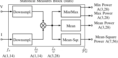
[image:5.612.315.564.55.240.2]

Having explored various methods for implementing the statistical measures and the underlying arithmetic, those ideas will be brought together. The details of the algorithm as it will be implemented in VHDL will be discussed, with especial focus on the design of the accumulators which are central to the calculation and number formats used. As mentioned, this implementation will serve as a proof-of-concept for the full block that would take all eight loop filter inputs. The block diagram of this algorithm is given in Figure 7, the sample rates are given below, where F N_w. The other blocks are shown in Figures 8 to 10, based on the mathematics behind each statistic. For all parts of the algorithm, the number formats at each stage are also indicated. Even though fixed point number formats are used, the arithmetic is the same as for two’s complement integers while keeping careful track of the position of the virtual decimal point.

Fig. 6. Comparison of percentage error and computational complexity of various window sizesw(represented in frames of 512 samples) using mean-square calculation. The songs used are of various genre and compression levels.

Downsmpl. V

Downsmpl. I

Min Power A(3,28) Max Power

A(3,28)

Mean Mean Power_A(3,28)

Mean-Sqr. _{Power A(7,56)}Mean-Square Min/Max

Statistical Measures Block (stats)

fs fs_w fs_w _{F w}fs

A(1,14) A(1,14) A(3,28)

Fig. 7. Block diagram of Statistical Measurements algorithm. Sample rates and number formats indicated below.

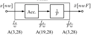
A. Downsampling

The downsampling block is shown in Figure 8. The sum-mation of the mean used in downsampling, as used in (5), is achieved using an accumulator (Acc.). The inputs to the accumulator are both positive and negative, centred around zero. Thus, it is expected that the output value of the accumu-lator is in the same range as the input, however consecutive positive or negative values need to be taken into account so that these do not cause an overflow. Due to the upsampled nature of the signals, there will always be at least 512 consecutive values with the same sign. As explained above, in order to avoid an overflow the number format of the accumulator will have to be A(r1 log2p1024qs,14)=A(11,14). There is only one clock cycle to complete each addition, therefore addition in the downsampling block will be implemented parallelly. Since the downsampled approximation is expected to have the same range as the input, the number format after division can be the same as the input format, A(1,14). The division itself is done with a virtual bit shift by log2w, and then

[image:5.612.315.556.310.428.2]

(6)

Downsample

xrns

Acc. _w1

¯ xrnws

fs f_ws f_ws

[image:6.612.343.539.59.126.2]

A(1,14) A(11,14) A(1,14)

Fig. 8. Block diagram of Downsampling algorithm. Sample rates and number formats indicated below.

B. Multiplier

The multiplication after downsampling will be implemented serially, since there are w clock cycles to do the operation before the next frame. In order to avoid overflow or precision loss the output format will be 32-bit A(3,28) [10]. When only one input signal is used (for example voltage), this has to be converted from A(1,14) to A(3,28) by sign extension before going into the following blocks, as it would otherwise require different hardware to do computations on this number format.

C. Mean

The mean block is similar to the downsampling block. It is shown in Figure 9. The accumulator in this block will be serial however, as there are w clock cycles per addition. The input is A(3,28) from the multiplier. The accumulator addsFinputs rather thanw. Due to this, the required number format of the accumulator will be A(3 log2p216_q_{,28)=A(19,28). Division is}

done similarly to the downsampling block as well, this time shifting by log2pFq and keeping 32 bits to match the input number format.

Mean

xrnws

Acc. _F1

¯ xrnwFs fs

w

fs F w

A(3,28) A(19,28) A(3,28)

Fig. 9. Block diagram of Mean algorithm. Sample rates and number formats indicated below.

D. Mean-Squared

The mean-square block is shown in Figure 10. The square will be implemented similarly to the multiplier already dis-cussed. The number format of the square will be A(7,56) to allow for the maximum value and avoid loss of precision. The accumulator will have to have number format A(23,56) and be implemented serially like in the mean block. The division will again be done with a virtual shift by log2pFq as previously described, resulting in an output format the same as the input format to the accumulator A(7,56).

E. Comparator

Both the input and output formats of the comparator are A(3,28). The comparator will be implemented serially as described in Section IV-D. Since the input is 32-bit, the comparator will take at most 64 clock cycles to complete.

xrnws

x2 _Acc. 1

F ¯ x2_r_{nF w}_s Mean-Sqr.

fs w

fs F w

[image:6.612.318.557.195.359.2]

A(3,28) A(7,56) A(23,56) A(7,56)

Fig. 10. Block diagram of Mean-Square algorithm. Sample rates and number formats indicated below.

TABLE II

AREA OF ALGORITHMBLOCKS

Block Area 65nm(µm2₎ _{Area 55nm}₍_µ_m2₎ _Slack_(ns)

Total (stats) 12249 9922 34.392

ëDownsample 629 509

ëAccumulator 629 509

ëAdder 193 156

ëMultiplier 1772 1435

ëMean 1131 916

ëAdder 438 355

ëMean-Sqr. 6268 5077

ëSquare 4481 3630

ëAdder 678 549

ëComparator 1451 1175

F. Synthesis

The amplifier controller is manufactured on a 55nm process. However, due to the non-availability of synthesis libraries for this process, UMC 65nm is used. Scaling area between the process nodes is straightforward, as 55nm is a half node shrink from 65nm. To convert from 65nm to 55nm each dimension scaled by a factor of 0.9; a total factor of 0.81.

VI. RESULTS

The VHDL code for each of the algorithm blocks is given in Appendix A. The blocks are created in a modular fashion to allow future expansion. Unfortunately, out of time constraints default library implementations of addition (+), multiplication (*) and comparison ( ,¡) are used rather than specific serial implementations. The size of each of the synthesised blocks is presented in Table II. The area of sub-blocks is for that individual block, not the sum of all instances of the block For example, the downsampling block is actually implemented twice; once for voltage, once for current, but not represented twice in the table. The slack of high level blocks is also measured, using a clock period of ₅₁₂_48kHz1 40.69ns. Unfortunately, serial arithmetic has not been implemented, resulting in a larger area.

VII. DISCUSSION ANDFURTHERRESEARCH

[image:6.612.100.253.438.497.2]

(7)

using serial multiplication results in the majority of the area of the algorithm coming from the multiplication and square blocks. Without implementing serial multiplication, the only way to reduce the area would be to sacrifice precision and discard LSB’s as is done with division. Division does discard some values, log₂w or log₂F, depending on where it is implemented, reducing precision. However, for the presented application, where a downsampled approximation of the input signal is central to the design, it is questionable whether the error introduced by rounding is significant at all. More precise tuning could be done depending on the accuracy required by the output and the size of the accumulators. It would be possible to keep the word length at 16-bits throughout, while losing precision at every step. Another feature that sticks out is how often certain blocks are repeated, especially the accumulator and adder. Sharing the accumulator between blocks would already result in a decrease of total area. The latency introduced by this is not expected to be an issue, as there is a lot of slack time left per clock cycle.

Since the algorithm developed in this report only serves as a proof-of-concept, there are many opportunities to continue research on the topic. First and foremost, an implementation of serial addition, comparing and especially multiplication would make a dramatic difference. Dedicated arithmetic for performing the square operation which is more efficient than regular multiplication may also reduce computational com-plexity. With the number of possibilities there are for a comparator implementation, more investigation could be done in to the most optimal configuration for a comparator. Another drawback of the current implementation is that each arithmetic block is implemented separately. Sharing resources such as the accumulation logic between Mean and Mean-Square and between both downsampling blocks would reduce the size of the total algorithm. With respect to the number formats, and the number of bits used, a statistical analysis on the input signal may be useful to be able to better predict the range of data at each stage of the input, thus reducing the number of bits used at each operation. The maximum value of the accumulators (α2a_{), as presented in Section IV-E, will almost} certainly never be reached for an audio signal, meaning bits are wasted. While optimising the number of bits, however, the design of the arithmetic units should be taken into account. The serial arithmetic may be based on two- or four-bit blocks and should be compatible with the number of bits used to represent values. In terms of the real-life application of the algorithm, the proof-of-concept algorithm presented in Figure 7 can be expanded to work on 8 input signals, pairs of any of which could be used for power calculations.

VIII. CONCLUSION

The proof-of-concept algorithm designed provides a good platform for further investigation and design of the full algo-rithm. Downsampling using the mean has clear advantages in reducing computational complexity, and can be simply implemented. Completely eliminating the need for division greatly reduces complexity and area of the algorithm. While

the implemented proof-of-concept has inefficient use of area, techniques are presented that could be immediately imple-mented in an update to this design, using serial arithmetic and effective sharing of algorithmic blocks.

REFERENCES

[1] R. Veldhuis, “Sampling-Rate Conversion,” inLecture Notes Discrete-Time Signal Processing, May 1, 2018 ed., Enschede, 2018, ch. 7, pp. 85–101.

[2] S. F. Ismael and B. Shukr, “A Novel Way to Design and

Implement Statistical Operations based on FPGA,” International

Journal of Computer Applications, vol. 167, no. 9, pp. 8– 11, jun 2017. [Online]. Available: http://www.ijcaonline.org/archives/ volume167/number9/ismael-2017-ijca-914359.pdf

[3] M. Murdocca and V. P. Heuring,Computer Architecture and Organiza-tion: An Integrated Approach. New Jersey: John Wiley & Sons, Inc., 2007.

[4] M. Vl˘adut¸iu, Computer Arithmetic, 1st ed. Berlin, Heidelberg: Springer-Verlag Berlin Heidelberg, 2012. [Online]. Available: http: //link.springer.com/10.1007/978-3-642-18315-7

[5] A. A. Mallya, A. S. B, F. J. Sequeira, S. Hebbar, and D. Divakar, “FSM Serial Adder,” International Journal of Latest Technology in Engineering, Management & Applied Science, vol. V, no. VI, pp. 65–67, 2016.

[6] S. Shirani, “Serial Adder,” Ontario.

[7] J. Wakerly, “Combinational Logic Design Practices,” inDigital design: Principles and Practices. New York: Prentice-Hall, 2000, ch. 5, pp. 273–428. [Online]. Available: http://bida.uclv.edu.cu/bitstream/handle/ 123456789/9935/Criptogr.pdf?sequence=1t&uisAllowed=y

[8] A. Al-Khalili, “Parallel Adders,” Quebec.

[9] W. Stallings, “Computer Arithmetic,” in Computer Organization and Architecture : Designing for Performance, 8th ed. New Jersey: Prentice Hall, 2010, ch. 9, pp. 305–347.

[10] R. Yates, “Fixed-Point Arithmetic: An Introduction,” 2007. [Online]. Available: https://courses.cs.washington.edu/courses/cse467/08au/labs/ l5/fp.pdf

[11] M. Morris Mano, Digital Logic And Computer Design By, 2nd ed.

Englewood Cliffs: Prentice-Hall.

(8)

APPENDIXA VHDL CODE

A. Statistical Measurements (stats)

1LIBRARY IEEE;

2USE IEEE.std_logic_1164.ALL;

3USE IEEE.numeric_std.ALL;

4

5ENTITY stats IS -- top block

9 | | |log2F : integer :=16); -- log2 of window size 10 |PORT (clk , reset: IN std_logic;

11 | |v,i: IN signed(15 downto0); -- voltage, current stream 12 | |psel: IN std_logic; -- select power or voltage

16 | |meansqrOut: OUT signed(63 downto 0) ); -- mean-square 17 END ENTITY stats;

18

19 ARCHITECTURE bhv of stats IS

20 |SIGNAL clk2 : std_logic; -- clock for F, 'slower blocks' 21 |COMPONENT downsmpl IS -- approximation block

22 | |GENERIC(w: integer;

23 | | | |log2w: integer );

24 | |PORT(clk,reset: IN std_logic;

28

29 |COMPONENT mult IS -- multiplier

33

34 |COMPONENT mean IS -- mean block 35 | |GENERIC(F : integer;

36 | | | |log2F : integer );

41

42 |COMPONENT meansqr IS -- mean-sqr block 43 | |GENERIC(F : integer;

44 | | | |log2F : integer );

49

50 |COMPONENT comp IS -- compare block 51 | |GENERIC(F : integer);

53 | | |x : IN signed (31 downto 0); --A(3,28)

54 | | |maxi,mini : OUT signed(31 downto 0) ); --A(3,28) 55 |END COMPONENT;

56

57 |SIGNAL vApp,iApp : signed(15 downto 0); -- A(1,14) 58 |SIGNAL pApp,vtmp,app : signed(31 downto 0); -- A(3,28) 59 |SIGNAL clktmp : std_logic := '0';

60 |SIGNAL reset1 : std_logic; -- reset for 'slower blocks' 61 BEGIN

62 |PROCESS(clk,reset) -- clock divider 63 | |VARIABLE counter : integer range 0 to w;

64 |BEGIN

65 | |IFreset = '1' THEN

66 | | |counter := 0;

67 | | |clktmp <= '0';

68 | |ELSIF rising_edge(clk) THEN

69 | | |counter := counter + 1;

70 | | |IF counter = w/2 THEN

71 | | | |clktmp <= NOT clktmp;

72 | | | |counter := 0;

73 | | |END IF;

74 | |END IF;

75 | |clk2 <= clktmp;

76 |END PROCESS;

77

78 |PROCESS(clk) -- reset for slower

79 | |VARIABLE c : integer range 0 tow; -- blocks. Waits for

80 |BEGIN -- first downsample

81 | |IFreset ='1' THEN -- to complete

82 | | |c := 0;

83 | |ELSIF c < w THEN

84 | | |c := c + 1;

85 | | |reset1 <='1';

86 | |ELSE

87 | | |reset1 <='0';

88 | |END IF;

89 |END PROCESS;

90

91 |approxV : downsmpl GENERIC MAP(w =>w, log2w => log2w)

92 | | | | | |PORT MAP(clk => clk, reset => reset,

93 | | | | | | | |xExact => v, xApp => vApp);

94 |approxI : downsamp GENERIC MAP(w =>w, log2w => log2w)

95 | | | | | |PORT MAP(clk => clk, reset => reset,

96 | | | | | | | |xExact => i, xApp => iApp);

97 |VItoP : mult PORT MAP(a => vApp, b => iApp, y => pApp);

98 |

99 |vtmp(28 downto 14) <= vApp(14 downto 0); -- Format v 100 |vtmp(31 downto 29) <= (others => vApp(15));|-- as A(3,28) 101 |

102 |app <=|pApp WHEN psel = '1' ELSE -- power calculations 103 | | |vtmp WHEN psel = '0'; -- voltage calculations 104

105 |meansqr1 : meansqr GENERIC MAP(F =>F, log2F => log2F)

106 | | | | |PORT MAP(clk => clk2, reset => reset1,

107 | | | | | | |x => app, y => meansqrOut);

108 |mean1 : mean GENERIC MAP(F => F, log2F => log2F)

109 | | | | |PORT MAP(clk => clk2, reset => reset1,

110 | | | | | | |x => app, y => meanOut);

111 |comp1 : comp GENERIC MAP(F => F)

112 | | | |PORT MAP(clk => clk2, reset => reset1,

113 | | | | | |x => app, mini => mini, maxi => maxi);

114 END ARCHITECTURE bhv;

B. Downsampling

1 ENTITY downsmpl IS

2 |GENERIC(w: integer;

3 | | |log2w: integer);

4 |PORT(clk,reset: IN std_logic;

5 | |xExact : IN signed(15 downto 0); -- A(1,14) 6 | |xApp : OUT signed(15 downto 0) ); -- A(1,14) 7 END ENTITY downsmpl;

8

9 ARCHITECTURE bhv ofdownsmpl IS

10 |COMPONENT accumulator IS

11 | |GENERIC(w,inBits,outBits: integer);

12 | |PORT(clk, reset : IN std_logic;

13 | | |x : IN signed(15 downto 0); -- A(1,14)

14 | | |y : OUT signed(15+log2w downto 0) ); -- A(11,14) 15 |END COMPONENT;

16

17 |SIGNALxAcc : signed(15+log2w downto 0); -- A(11,14) 18 BEGIN

19 |acc: accumulator GENERIC MAP(w => w, inBits => 16,

20 | | | | | | | |outBits =>16+log2w)

21 | | | | |PORT MAP(clk => clk,reset=>reset,

22 | | | | | | |x => xExact, y => xAcc);

23 |xApp <= xAcc(15+log2w downto log2w); -- divide A(1,14) 24 END bhv;

C. Accumulator

1 ENTITY accumulator IS

2 |GENERIC(w : integer;

3 | | |inBits,outBits : integer);

4 |PORT(clk, reset : IN std_logic;

5 | |x : IN signed(inBits-1 downto 0);

6 | |y : OUT signed(outBits-1 downto 0) );

7 END accumulator;

8 ARCHITECTURE bhv ofaccumulator IS

9 |SIGNALreg : signed(outBits-1 downto 0); -- acc. resister 10 BEGIN

11 |PROCESS (clk, reset)

12 | |VARIABLE count : integer range 0 to w;

13 |BEGIN

14 | |IF (reset='1') or count = w THEN

15 | | |y <= reg;

16 | | |reg <= (others => '0');

17 | | |count := 0;

19 | | |reg <= reg + x;

20 | | |count := count + 1;

21 | |END IF;

22 |END PROCESS;

(9)

D. Multiplier

1ENTITY mult IS

2 |PORT(a,b : IN signed(15 downto 0); -- A(1,14) 3 | |y : OUT signed(31 downto0) ); -- A(3,28) 4END mult;

5ARCHITECTURE bhv of mult IS

6BEGIN

7 |y <=a*b;

8END bhv;

E. Mean

1ENTITY mean IS

2 |GENERIC(F : integer;

3 | | |log2F : integer);

5 | |x : IN signed(31 downto 0); --A(3,28) 6 | |y : OUT signed(31 downto0) ); --A(3,28) 7END mean;

8

9ARCHITECTURE bhv of mean IS

13 | | |x : IN signed(31 downto 0); --A(3,28)

14 | | |y : OUT signed(31+log2F downto 0) ); --A(19,28) 15 |END COMPONENT;

16

17 |SIGNAL xAcc : signed(31+log2F downto 0); --A(19,28) 18 BEGIN

19 |acc: accumulator GENERIC MAP(w =>F, inBits => 32,

20 | | | | | | | |outBits => 32+log2F)

22 | | | | | | |x => x, y => xAcc);

23 |y <=xAcc(31+log2F downto log2F); -- divide A(3,28) 24 END bhv;

F. Mean-Sqr.

1ENTITY meansqr IS

2 |GENERIC(F : integer;

3 | | |log2F : integer );

5 | |x : IN signed(31 downto 0); --A(3,28) 6 | |y : OUT signed(63 downto0) ); --A(7,56) 7END meansqr;

8

9ARCHITECTURE bhv of meansqr IS

10 |COMPONENT sqr IS

17 | | |x : IN signed(63 downto 0); --A(7,56)

18 | | |y : OUT signed(31+log2F downto 0) ); --A(23,56) 19 |END COMPONENT;

20

21 |SIGNAL xsqr : signed(63 downto 0); --A(7,56) 22 |SIGNAL xAcc : signed(63+log2F downto 0); --A(23,56) 23 BEGIN

24 |sqr1 : sqr PORT MAP(x => x, y => xsqr);

25 |acc: accumulator GENERIC MAP(w =>F, inBits => 64,

26 | | | | | | | |outBits => 64+log2F)

28 | | | | | | |x => xsqr, y => xAcc);

29 |y <=xAcc(63+log2F downto log2F); -- divide A(7,56) 30 END bhv;

G. Square

1ENTITY sqr IS

2 |PORT(x : IN signed(31 downto 0); -- A(3,28) 3 | |y : OUT signed(63 downto0) ); -- A(7,56) 4END sqr;

5ARCHITECTURE bhv of sqr IS

6 |SIGNAL tmp : signed(63 downto 0);

7BEGIN

8 |y <=x*x;

9END bhv;

H. Min/Max (Comparator)

1 ENTITY comp IS

2 |GENERIC(F : integer);

4 | |x : IN signed (31 downto 0); --A(3,28)

5 | |maxi,mini : OUT signed(31 downto 0) ); --A(3,28) 6 END comp;

7

8 ARCHITECTURE bhv ofcomp IS

9 |SIGNALmaxMem, minMem : signed(31 downto 0);

10 BEGIN

11 |PROCESS(clk,reset)

12 | |VARIABLE count : integer range 0 to F;

13 |BEGIN

14 | |IF reset = '1' OR count = F THEN

15 | | |mini <= minMem;

16 | | |maxi <= maxMem;

17 | | |maxMem <=(others => '0');

18 | | |minMem <=(others => '0');

19 | | |count := 0;

21 | | |IFx > maxMemTHEN

22 | | | |maxMem <= x;

23 | | |ELSIF x < minMem THEN

24 | | | |minMem <= x;

25 | | |END IF;

26 | | |count := count + 1;

27 | |END IF;

28 |END PROCESS;