Data mining for vehicle telemetry

warwick.ac.uk/lib-publications

Taylor, Phillip, Griffiths, Nathan, Bhalerao, Abhir, Anand, Sarabjot Singh, Popham, T. J., Xu, Zhou and Gelencser, Adam. (2016) Data mining for vehicle telemetry. Applied Artificial Intelligence, 30 (3). pp. 233-256.

Permanent WRAP URL:

http://wrap.warwick.ac.uk/78813 Copyright and reuse:

The Warwick Research Archive Portal (WRAP) makes this work by researchers of the University of Warwick available open access under the following conditions. Copyright © and all moral rights to the version of the paper presented here belong to the individual author(s) and/or other copyright owners. To the extent reasonable and practicable the material made available in WRAP has been checked for eligibility before being made available.

Copies of full items can be used for personal research or study, educational, or not-for profit purposes without prior permission or charge. Provided that the authors, title and full bibliographic details are credited, a hyperlink and/or URL is given for the original metadata page and the content is not changed in any way.

Publisher’s statement:

“This is an Accepted Manuscript of an article published by Taylor & Francis in Applied Artificial Intelligence on 2016 available online:

http://www.tandfonline.com/10.1080/08839514.2016.1156954 A note on versions:

The version presented here may differ from the published version or, version of record, if you wish to cite this item you are advised to consult the publisher’s version. Please see the ‘permanent WRAP url’ above for details on accessing the published version and note that access may require a subscription.

Phillip Taylor

, Nathan Griffths

, Abhir Bhalerao

, Sarabjot Anand

,

Thomas Popham

, Zhou Xu

, and Adam Gelencser

1

_{Dept. of Computer Science, The University of Warwick, Coventry, UK}

2

_{Algorithmic Insight, New Dehli, India}

3

_{Jaguar Land Rover Research, Coventry, UK}

Abstract

This paper presents a data mining methodology for driving condition

moni-toring via CAN-bus data that is based on the general data mining process. The

approach is applicable to many driving condition problems and the example of

road type classification without the use of location information is investigated.

Lo-cation information from Global Positioning Satellites and related map data are

often not available (for business reasons), or cannot represent the full dynamics

of road conditions. In this work, Controller Area Network (CAN)-bus signals are

used instead as inputs to models produced by machine learning algorithms. Road

type classification is formulated as two related labelling problems: Road Type (A,

B, C and Motorway) and Carriageway Type (Single or Dual). An investigation

is presented into preprocessing steps required prior to applying machine learning

algorithms, namely, signal selection, feature extraction, and feature selection. The

selection methods used include Principal Components Analysis (PCA) and Mutual

Information (MI), which are used to determine the relevance and redundancy of

extracted features, and are performed in various combinations. Finally, as there is

an inherent bias towards certain road and carriageway labellings, the issue of class

imbalance in classification is explained and investigated. A system is produced,

which is demonstrated to successfully ascertain road type from CAN-bus data, and

it is shown that the classification correlates well with input signals such as vehicle

speed, steering wheel angle, and suspension height.

Keywords: Data mining, Driving condition monitoring,

Feature selection, Road classification

1

Introduction

Driving conditions monitoring aims to detect parameters about the road and a vehi-cle’s surroundings (Huang et al., 2011), such as the road surface, level of congestion, or weather. Knowledge of the current driving conditions can have several benefits: user interface adaptation, engine power management, and driver monitoring (Huang et al., 2011; Langari and Won, 2005; Murphey et al., 2008; Park et al., 2008); all of which strive to improve driver safety and vehicle efficiency. In this paper we present a data mining methodology, based on the general data mining process, for driving condition monitoring via Controller Area Network (CAN)-bus data. Two related classification problems are considered, Road Type labelling (into types A, B, C and Motorway) and Carriageway Type labelling (into types Single or Dual). Road Type labelling aims to detect the state or governmental designation of roads from vehicle telemetry data. Using the same inputs, Carriageway Type labelling aims to detect whether the vehicle is being driven on a single or dual (or multi) track road.

In some instances, the road type can be determined with location and map data using Global Positioning Systems (GPS). However, although in principle it is an accurate system, it can be impractical or unsuitable because in many vehicles and locations, GPS signals are unavailable, or access to digital maps is costly and unreliable, and map data may be unavailable or outdated for a region. Another issue with digital map data with state road type designations is that these may not be reflective of the current driving conditions. In the UK, for example, class A roads can be fast dual carriageway roads in the countryside as well as restricted speed single track roads in congested urban areas. Furthermore, location information does not take into account changes in traffic flow, which may fluctuate throughout the day and is affected significantly by accidents and roadworks. For these reasons it can be preferable to make a business decision to exclude GPS data for certain driving conditions monitoring applications.

in the vehicle can be recorded and post-processed in order to sample sensor measurements at a certain frequency. Our proposed classification system uses machine learning, in a data mining framework, to correlate CAN-bus signals to pre-learned class labels, such as road types. With this approach, sudden and unexpected changes in driving conditions on a road can be taken into account, which is not possible when using location data with-out external data sources. If an accident significantly affects the driving conditions on a motorway, for example, a model based on speed and suspension measurements should be able to change its output appropriately.

CAN-bus data consists of thousands of signals sampled at high frequencies for hours at a time, generating very large datasets. Selecting which signals, and features of signals, to use is a challenging task, with engineers often hand picking model inputs from thou-sands of signals (Taylor et al., 2012). This manual selection, as well as being tedious, can introduce deficiencies into systems, as selection may be due more to an engineer’s knowl-edge and preferences rather than the true usefulness of a signal. In this work, we also propose an automatic feature selection framework which might aid engineers in building better models for environment monitoring problems in general.

This paper makes the following key contributions:

• A methodology, based on the general data mining process (John, 1997), is presented for driving conditions monitoring problems such as road classification.

• Two related temporal classification problems are presented, using data collected from two cars with multiple drivers over 16 journeys. This provides a strong evalu-ation framework where models are tested on data from different journeys to those that were used to build them.

• An approach to the pre-processing of CAN-bus data is developed; including signal selection, feature extraction and feature selection.

• The methodology is applied to create a system that is able to successfully detect the current road type in real time, using only 2.5 seconds of historical data.

process are described in Section 4, including the feature extraction and selection processes used. The results of our investigations are then presented in Section 5. Finally, in Sections 6 and 7, we discuss the results, draw conclusions and identify future steps.

2

Related work

Data mining of CAN-bus data has been used in several applications, including fault de-tection (Crossman et al., 2003; Guo et al., 2000), driver monitoring (Mehler et al., 2012; Taylor et al., 2013b), and driving conditions monitoring, which is surveyed by Wang and Lukic (2011) and is the focus of this paper. Fault detection aims to determine whether there is a vehicle failure and what may have caused the it. Whereas fault detection is usu-ally performed offline in a workshop, driver monitoring and driving conditions monitoring operate while the vehicle is being driven. For instance, they aim to predict parameters about the driver and their surrounding environment, so that the driver interface can be adapted or the engine tuned.

In fault detection, both Guo et al. (2000) and Crossman et al. (2003) successfully apply wavelet analysis to split telemetry signals into segments, from which several features are extracted. The extracted features include the segment length, minimum and maximum values, as well as averages and fluctuations. A fuzzy rule classification algorithm is then used to determine whether the original signal was normal, or abnormal and indicative of a fault.

was used in Artificial Neural Networks, Decision Drees, and Support Vector Machines, achieving comparable performances.

In this paper, we consider the driving conditions monitoring problem of road classi-fication. Whereas driver monitoring focusses on driver state inside the vehicle, driving conditions problems relate to the outside environment, including the traffic levels, and road type (Huang et al., 2011; Langari and Won, 2005; Wang and Lukic, 2011). Driving conditions and road type can be defined in several ways, including level of service (Carl-son and Austin, 1997; Langari and Won, 2005; Murphey et al., 2008), descriptive (Haupt-mann et al., 1996; Huang et al., 2011; Qiao et al., 1995; Tang and Breckon, 2011; Taylor et al., 2012), and government classification (Taylor et al., 2012). Possibly the most used definition in research is that provided by Carlson and Austin (1997), based on level of service and driving cycles. Level of service and driving cycles are qualitative measures describing observed operational conditions (Langari and Won, 2005), and therefore may be subjective. Descriptive definitions are of most use, as they have a direct relationship to the current situation and environment. For example, Huang et al. (2011) use the la-bels highway, urban road (both congested and flowing), and country road. Hauptmann et al. (1996) use an even more direct classification structure, based upon current car behaviour. Their five labels range from very fast, straight line driving on flat roads, to very low speeds or stop. These are used to represent further driving situations, such as highway driving, and traffic lights or parking.

Other authors have used different features in addition to those extracted from speed cycles. Hauptmann et al. (1996), for example utilize engine speeds, accelerations, and gradient. Additionally, Qiao et al. (1995) extract features from the pedal positions, temperatures and selected gear. These features, however, although they contain different information from the vehicle speed, are all related to it. Engine speed, for example, has a Pearson correlation with vehicle speed of 0.96 on data we have collected, meaning that it is adding little new information into the system. Qiao et al. (1996) note that the length of the temporal window that features are extracted over is an important factor in the system’s reaction time and they use a much smaller window length of 6.25 seconds. One shortfall in their work, however, is that automatic feature selection is not performed and features are selected based on the intuition of the researchers.

Examples of feature selection being used in this domain are mainly those that use features extracted from speed cycles. Murphey et al. (2008) and Park et al. (2008) proposed a selection procedure based on binary class separability of single features: if a feature is able to distinguish one class label from the others, then that feature is selected. Huang et al. (2011) also use a non-parametric, one-way analysis of variances to ensure that features used are relevant, and use cross correlation analysis to remove redundancy. They investigate 11 features in total, with only 4 being manually selected for classification. When dealing with CAN-bus data, however, the number of signals and features can be in the order of 1000 seconds, meaning automatic approaches are necessary (Taylor et al., 2013a).

3

Data mining methodology

The methodology we present is based on a general framework for data mining outlined by John (1997). As in (Huang et al., 2011; John, 1997), and others, we use the term

data mining to refer to the process of collecting, processing, and learning from data as a whole. The methodology presented in this paper is of a similar form to those found in many temporal data mining applications, including (Constantinescu et al., 2010; Huang et al., 2011; Kargupta et al., 2004; Manimala et al., 2012; Sagheer et al., 2006; Shaikh et al., 2011; Wollmer et al., 2011) and others, and is split into stages of: data collection; feature extraction; feature selection; classification and evaluation. In this paper, we also consider selection of signals, prior to feature extraction. This has the advantage of saving computation, as only selected signals have to be processed later in the data mining process.

3.1

Data collection

The data collection must be planned carefully for data mining to be successful. First, the conditions under which data is to be collected, as well as what data should be recorded must be decided. It is important to control the acquisition conditions so that results become meaningful. Deciding on which data to record from vehicle telemetry is non-trivial, because of the thousands of signals available via the CAN-bus (Farsi et al., 1999). Recording and analysing all of them is an impossible task, so most researchers make educated guesses based on domain knowledge.

Second, the data representation should be in a form that is suitable for subsequent processing. For instance, the CAN-bus is an event based communications network where sensors broadcast data at varying rates (Farsi et al., 1999), so consequently, some data mining methods will not be directly applicable. It is typical therefore to re-sample the data at a common rate, e.g. between 10−100Hz, producing M signals, S1, S2, . . . , SM,

with samples of the same frequency.

later processing (Huang et al., 2011). Treating the data in this way, however, ignores any transition periods where a label change occurs. This may cause an evaluation to prefer models that use large amounts of historical data, but have slow reactions to changes in environment. In this paper, we consider the more realistic scenario of journeys which contain several periods of differing labels. Although this introduces noise during label changes, we believe this approach will provide more accurate performance estimates that do not ignore these reaction times.

3.2

Feature extraction

In temporal data mining, it is advantageous to include historical information when per-forming classification (Antunes and Oliveira, 2001). Without this, an individual sample contains only information about the exact point that sensor measurements were made, which may be noise. This means that no trend or statistical information can be used in determining the classification. We refer to this process of incorporating historical information into the current sample as temporal feature extraction.

Consider a signal, S, of lengthT, such as the vehicle speed or SWA.

f(S(t), S(t−1), ..., S(t−l+ 1)) =f(S(t, l)),

where f(S(t, l)) is a temporal summary of the values between times t and t−l+ 1. If

t < l, because it is at the beginning of the recorded signal, t samples are used. Features can generally be split into two categories, namely structural and statistical. Structural features describe the trend of the signals, whereas variations, peaks, and averages are represented by statistical features.

In each time instance,msignals,S1(t), S2(t), ..., Sm(t) are sampled, from each of which k features, f1, f2, ..., fk are extracted. Therefore, after feature extraction, a sample, x(t),

at timet, is represented as,

x(t) = {f1(S1(t, l)), ..., f1(Sm(t, l));

f2(S1(t, l)), ..., f2(Sm(t, l));

...;

It should be noted here that in some cases, different features may be extracted over different temporal windows from each signal, meaning that the value ofk and lmay vary between signals and features in the same dataset. Finally, whereas Huang et al. (2011) extract features from windows with no overlap, in this paper features are extracted over sliding windows with an overlap of l−1. This means that a temporal dataset of length

T, is a sequence of samples,

X =x(1), x(2), ..., x(T −1), x(T).

This method both maximizes the number of samples and means their number is not dependent on window length. The overlap in windows does increase the autocorrelation in the data, however, which can be problematic for some data mining methods.

3.3

Signal and Feature selection

As previously stated, signals and features are often hand selected using domain knowl-edge. This is sub-optimal and time consuming, however, and may introduce biases toward the engineer’s preferences. We therefore use automatic selection of both signals, prior to feature extraction, and features, after feature extraction. We consider two common fea-ture selection methods, Principal Component Analysis (PCA), an unsupervised method for redundancy feature selection, and Mutual Information (MI), a supervised method for relevancy feature selection (Witten and Frank, 2005).

PCA transforms a dataset onto a set of orthogonal dimensions which are linearly uncorrelated, referred to as principal components (PCs) (Witten and Frank, 2005). This is done through computing Eigen values from the covariance matrix of the data. The idea is that because the dimensions produced are linearly uncorrelated, there is very little redundancy in the dataset. Also, if the PCs with the highest variance are selected (i.e. those associated with the largest Eigen values), they are also likely to contain the highest entropy and be good predictors.

Whereas PCA is an unsupervised method of feature selection, MI takes into account relationships between features and the class labels. MI is defined as,

M I(fi, C) =

X

vi∈vals(fi), vc∈vals(C)

p(vi, vc) log2

p(vi, vc) p(vi)p(vc)

where fi is a feature and C is the class labels. A high MI indicates that the feature is a

good predictor of the class labels and that it should be included in a predictive model. Both of these feature selection methods are able to provide a ranking of features. PCA ranks the PCs by their variance, where those with a larger variance are ranked higher. With MI, features are ranked by the closeness of their relationship with class labels.

3.4

Classification

In this paper, we employ three widely used machine learning algorithms: Na¨ıve Bayes, Decision Tree, and Random Forest, that are all available in the Waikato Environment for Knowledge Analysis (WEKA) machine learning suite (Witten and Frank, 2005). The Na¨ıve Bayes algorithm learns class conditional distributions from the data and uses Bayes rule to make inferences. For the Decision Tree classifier, we use the C4.5 algorithm which splits nodes based on MI. Once the full tree is built, pruning of nodes with few applicable samples is performed to prevent over-fitting. The Random Forest algorithm builds several Decision Trees, each on different sub-samples of the data and sub-sets of features. Each of these algorithms are chosen because of their wide-spread use and the ease with which models produced by them can be understood by a domain expert.

In road classification, there is an inherent class imbalance where one or more class labels dominate the training data. For example, there is a 5:1 ratio of single lane road ex-amples to multiple lane roads, and a smaller number of motorways than other road types in our data. This imbalance can lead to biases in models, which tend to prefer to label instances that are a majority (He and Garcia, 2009). We consider two approaches to deal-ing with class imbalance, namely over-sampldeal-ing and under-sampldeal-ing. In over-sampldeal-ing, samples of the minority class label are duplicated to increase their representation, while in under-sampling, some proportion of the majority class samples are decimated. Dupli-cation and decimation is performed by selecting samples at random.

Class Code

A Road 1000111 B Road 0100100 C Road 0010010 Motorway 0001001

Table 1: Example exhaustive coding for Road classification.

of the bits in these codes, i.e. there will be as many models as there are bits in the codes. In this example, the classifier predicting the third digit of the codes would predict 1 for C roads, and 0 for the remainder. The true code with the smallest Hamming distance between itself and the predicted code is then output as the sample classification.

Some of the binary class models will have better performance than others, because of the difficulty of distinguishing the classes. A and B roads, for example, are much more closely related than C roads and Motorways, so we would expect a model distinguishing between A and B roads to have worse performance. Because of this, it is sometimes beneficial to take account of this in the Hamming distance calculation by weighting it with expected performance (Zhang et al., 2012). This is done by updating the Hamming distances by multiplying them by the expected performances and can be illustrated using the example in Table 1. Suppose, for example, that the expected success rate, estimated using the training data, for each of the dichotomies is W = [0.75,0.5,1,1,1,0.5,0.5]. If the base models then output a bit string of 1100101, the weighted Hamming distances would be 1, 1.25, 4.25, 3.25 for A road, B road, C road and Motorway respectively. With these distances, the output the classification is of type A road.

3.5

Evaluation

This is repeated for several combinations of training and testing data, producing a large number of predictions made by the models. These predictions are then compared against the ground truth to produce a performance metric. Because it is possible to use some samples multiple times in an evaluation, the performance metrics exhibit Monte Carlo variation.

Unlike other work in environment classification, we choose to not use accuracy or error rates as a measure of performance. Instead, in this paper we use Area Under the ROC (Receiver Operating Characteristic) curve (AUC), as it is better suited in situations with a high class imbalance (Huang and Ling, 2005). This is because the imbalance may bias the output of a classifier, which is not accounted for by accuracy. Consider a model that outputs a probability distribution over the class labels and trained with an imbalanced binary classification dataset with numerous times more 0 labels than 1s. When using accuracy, an output ofp(0) = 0.7, p(1) = 0.3 with a decision threshold of 0.5 would mean that the prediction is 0. In this case, a model that outputsp(0) = 1 for all inputs, always predicting 0, may provide a very high accuracy on the dataset due to this being correct for most of the samples. When used in the real world, however, predicting 0 regardless of the situation is not useful. The ROC curve accounts for any class biases by computing true positive and false positive rates over several thresholds, ranging from 0 to 1. A threshold of 1 for a class means that the class label is never predicted, producing no false negatives and no false positives. Conversely, a threshold of 0 would mean all instances are predicted as the class label, producing a false negative rate and false positive rate of 1. The true positives are then plotted on the y-axis against the false positives on the x-axis, with the ideal curve following the y-axis as close as possible, having an AUC of 1.

4

Experimental Setting

4.1

Data collection

but sampled at 20Hz using linear interpolation, a value change would produce some samples between 0 and 1. Also, using the last broadcast value ensures that the signal is as up-to-date as possible, although it may mean it is more susceptible to noise.

The data used in this paper was collected over 16 drives across the Midlands, UK, in two cars. Each journey involves at least one driver, with a mean journey length of 51 minutes. Output from 15 CAN-bus sensors, listed with brief explanations in Table 2, were recorded each at 20Hz for a total of 49403 seconds, which is comparable to the length of data used in (Huang et al., 2011). Some sensors used are expected to have very little relevance in determining the road type, and others are highly redundant. As previously stated, these expectations may be incorrect, as is the case with the ambient temperature signal. Although it may initially be expected to be a poor predictor, it has one of the higher MI scores (0.197 for carriageway type) in data we have collected. On further inspection we find that its Pearson correlation with vehicle speed, which is expected to be a good predictor, is 0.774. This makes some intuitive sense, as the temperature near the engine will rise with vehicle speed as the engine works harder. With this insight we can say that ambient temperature is a good predictor of road type, but that it is somewhat redundant to other signals. After signal and feature selection, only the features which are useful for the problem should be used in classification.

The ground truth for the dataset was achieved using GPS and applied by hand using Google Earth. GPS coordinates are looked up in Google Earth and a label is decided, and assigned to samples. For the carriageway classification, the number of lanes is decided by looking at the satellite images provided. If there is more than one lane, the sample is

dual, otherwise it is single. For road type, the road name is looked up on the map and the first letter taken. If no road name is provided, because it is a dirt track or car park, the label given is C. The distribution of labels is provided in Table 3.

4.2

Signal selection, feature extraction and feature selection

For temporal feature extraction, we use two statistical features, the mean,

fµ(s) =

1

|s|

|s|

X

i=1

Signal Description

Ambient temperature Outside temperature (measured behind grill). Brake pressure Pressure on brake pedal.

Gear position (Automatically) selected gear.

Longitudinal/lateral accelerations Forward and Side-to-side accelerations of the vehicle, measured by an accelerometer.

Suspension height (each wheel) Heights of suspension (Front-Right, Front-Left, Rear-Right and Rear-Left).

SWA Angle of steering wheel. SWA speed Rate of change of SWA.

Vehicle speed Vehicle speed (measured from wheel speed). Wiper status Speed status of the front window wipers.

Table 2: List of signals recorded.

Label Percent (%) Description

Single carriageway 85 Single lane roads

Dual carriageway 15 Roads with multiple lanes

A road 48 Town road or non-highway arterial roads

B road 26 Smaller town or country roads

C road 21 Other types of road and car parks

Motorway 5 Highway with multiple lanes

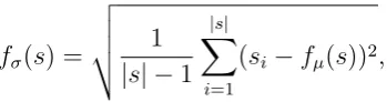
and standard deviation,

fσ(s) = v u u

t 1

|s| −1

|s|

X

i=1

(si−fµ(s))2,

wheres is a temporal window of the signal. We also use two structural features, the first and second derivatives, which are computed by taking the mean difference between each pair of points in the signal window,

δ(s) = [s2−s1, s3−s2, . . . , sl−sl−1].

The first derivative is then,

fδ1(s) = fµ(δ(s))

and second derivative is,

fδ2(s) =fµ(δ(δ(s))).

The standard deviation provides a measure of signal variance, while the derivatives pro-vide information on the gradient and shape of the signals. All four features are extracted from each signal with a window length of l = 2.5 seconds, or 50 samples. This length allows sufficient historical data for the features to be of use, while being small enough to be updated rapidly if the conditions change (Qiao et al., 1995). 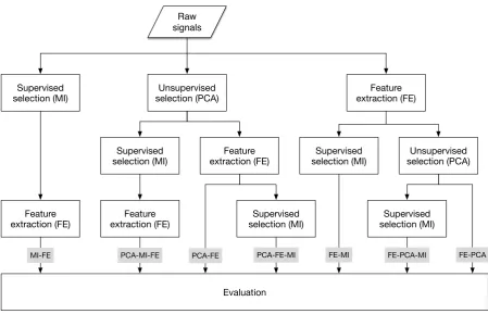Also, in a previous study, we have shown that a window length of over 2.5 seconds can not provide much increase in performance without causing over-fitting (Taylor et al., 2012).

In many cases of learning from CAN-bus data (Huang et al., 2011; Murphey et al., 2008; Taylor et al., 2013a; Wollmer et al., 2011), feature selection is performed after feature extraction has taken place. However, because of their number, selecting from the full set of extracted features is computationally prohibitive. It is beneficial to perform selection on signals prior to feature extraction, because there are fewer signals than total features. Therefore, we investigate signal selection prior to feature extraction and explore the impact combination of redundant and relevant feature selection.

Supervised

selection (MI) selection (PCA)Unsupervised extraction (FE)Feature

Evaluation Raw

signals

Supervised selection (MI)

Feature extraction (FE) Feature

extraction (FE)

Feature extraction (FE)

Supervised selection (MI)

Supervised

selection (MI) selection (PCA)Unsupervised

Supervised selection (MI)

MI-FE PCA-MI-FE PCA-FE PCA-FE-MI FE-MI FE-PCA-MI FE-PCA

Figure 1: Processing methods for data, for Principal Components Analysis (PCA), Mu-tual Information (MI) and Feature Extraction (FE). Some selection is performed on signals, prior to feature extraction. In this diagram, for example, the leftmost path of MI-FE first performs signal selection with MI, and then extracts features on the selected signals.

to feature extraction, which are then all input into the evaluation procedure. We refer to this particular path as MI-FE. Some paths are equivalent and are therefore omitted from our investigations. For instance, any path that has an MI stage followed by PCA is equivalent to performing solely PCA.

4.3

Classification and evaluation

sub-sampled by a factor of 10 at this point. Thirty models are then built using different numbers of the ranked features, (1,2, . . . ,30), and each are used to label the test dataset. As previously stated, each repetition of the non-random sub-set validations provide AUC values as measures of performance. These AUC values are then plotted against the number of features used in the repetition. It is expected that the AUC values will increase as additional features are added, plateauing and then decreasing after a certain number (Kohavi and John, 1997). A good feature ranking will have a high peak or plateau which appears with a small number of features. In order to compare feature rankings therefore, both the magnitude and location of the peaks are inspected.

As discussed above, Na¨ıve Bayes (Witten and Frank, 2005), Decision Tree (Witten and Frank, 2005), and Random Forest (Breiman, 2001) classification algorithms were used in this evaluation. The class imbalance problem was also tackled by using under-sampling and over-under-sampling for the binary classification task, and Weighted-ECOC for the multi-class classification task. For computational reasons, classifier parameters are not optimized, and the default options provided by WEKA are used (Witten and Frank, 2005). The results are discussed in the following section.

5

Results

In this section the results of the feature selection investigations are discussed, presenting AUC performances of the Na¨ıve Bayes, Decision Tree, and Random Forest models, for:

• Carriageway and road classification with no class imbalance techniques being ap-plied.

• Carriageway classification, having applied under-sampling and over-sampling to the training data.

• Road classification with Weighted-ECOC learning.

0 5 10 15 20 25 30 0.6

0.65 0.7 0.75 0.8 0.85 0.9

Number of Features

Accuracy

Threshold = 0.0 Threshold = 0.1 Threshold = 0.5 Threshold = 0.9

Figure 2: Plots showing mean accuracies of the 200 evaluation folds when using several decision thresholds for carriageway classification using Na¨ıve Bayes without using class imbalance techniques and with features selected by PCA-FE-MI. The error bars are 95% confidence intervals computed using the standard deviation of accuracies of the 200 evaluation folds.

probability of asingleis less than 0.9. The lines in this plot show the mean accuracies over the 200 folds performed in the evaluation, and the error bars for 95% confidence intervals computed on their standard deviation. In this example, a threshold of 0 provides a constant classification accuracy of 0.84, which is only bettered by using the threshold of 0.1. This 0 threshold means that the model will output single regardless of the input, which is not useful in the real world even though it achieves a high accuracy performance when compared to other thresholds. Therefore, when class imbalance is present, as is in our data, accuracy is not a good performance measure to use. ROC curves overcome this by computing error rates over many thresholds, and AUC then provides a measure of performance considering all thresholds.

0 5 10 15 20 25 30 0.4

0.45 0.5 0.55 0.6 0.65 0.7 0.75

Number of Features

A UC FE-MI FE-PCA-MI MI-FE FE-PCA PCA-MI-FE PCA-FE-MI PCA-FE

(a) Na¨ıve Bayes

0 5 10 15 20 25 30

0.4 0.45 0.5 0.55 0.6 0.65 0.7 0.75

Number of Features

A UC FE-MI FE-PCA-MI MI-FE FE-PCA PCA-MI-FE PCA-FE-MI PCA-FE

(b) Random Forest

Figure 3: Carriageway classification AUC values against number of features used in the (a) Na¨ıve Bayes and (b) Random Forest classifiers. Performance of the Na¨ıve Bayes and Random Forest models are comparable when considering the FE-MI and MI-FE selection paths. Other selection paths perform less well using Random Forest, and any selection path containing a MI stage has good performance with Na¨ıve Bayes.

are not presented because of its poor performance.

A similar pattern in the results is seen in the road classification AUC performances, shown in Figure 4. Again, the Na¨ıve Bayes classifier has the highest AUC performance overall, with those feature sets produced by a selection path including an MI stage achiev-ing at least 0.65 in AUC. One difference is that the FE-MI and MI-FE selection paths no longer produce the highest performing feature rankings. Instead, the highest AUC performance is given by performing an MI stage after a PCA stage, using either the PCA-FE-MI or PCA-MI-FE selection paths. The FE-PCA-MI selection path does not share this high performance, indicating that dealing with redundancy in the signals pro-vides better features in this classification task.

Na¨ıve Bayes Decision Tree Random Forest

FE-MI 0.724 (17) 0.571 (8) 0.711 (19) FE-PCA-MI 0.704 (15) 0.608 (3) 0.640 (23) MI-FE 0.717 (30) 0.571 (13) 0.715 (16)

FE-PCA 0.696 (30) 0.600 (28) 0.644 (28) PCA-FE-MI 0.725 (11) 0.629 (1) 0.664 (21) PCA-FE 0.681 (26) 0.625 (6) 0.655 (22) PCA-MI-FE 0.714 (14) 0.635 (2) 0.661 (29)

(a) Carriageway Type

Na¨ıve Bayes Decision Tree Random Forest

FE-MI 0.671 (30) 0.552 (10) 0.633 (30) FE-PCA-MI 0.659 (13) 0.607 (6) 0.631 (11) MI-FE 0.671 (26) 0.554 (2) 0.637 (28) FE-PCA 0.652 (30) 0.606 (19) 0.625 (20) PCA-FE-MI 0.682 (11) 0.628 (7) 0.653 (12)

PCA-FE 0.649 (26) 0.631 (22) 0.639 (26) PCA-MI-FE 0.670 (14) 0.638 (2) 0.650 (15)

(b) Road Type

0 5 10 15 20 25 30 0.4

0.45 0.5 0.55 0.6 0.65 0.7 0.75

Number of Features

A UC FE-MI FE-PCA-MI MI-FE FE-PCA PCA-MI-FE PCA-FE-MI PCA-FE

(a) Na¨ıve Bayes

0 5 10 15 20 25 30

0.4 0.45 0.5 0.55 0.6 0.65 0.7 0.75

Number of Features

A UC FE-MI FE-PCA-MI MI-FE FE-PCA PCA-MI-FE PCA-FE-MI PCA-FE

(b) Random Forest

Figure 4: Road-type classification AUC values against number of features used in the (a) Na¨ıve Bayes and (b) Random Forest classifiers. Na¨ıve Bayes has highest AUC per-formance with features selected by the PCA-FE-MI, while Random Forest has slightly worse AUC performance for all selection paths.

the Decision Tree classification algorithm over-fits the data and often to the top ranked features, which is not generally rectified by pruning.

For the carriageway classification task, the FE-MI selection path provides a very similar AUC performance, but for road type classification it is lower. This again indicates that redundancy feature selection is a necessary step for the highest performance in the multi-class problem. Also from these results, there is some indication that the selection paths that contain both a relevancy and a redundancy stage require fewer features than those that only have one or the other. This can be clearly seen in the road classification peak scores, where 11 – 15 features are needed for those with both PCA and MI, and over 20 are commonly required for other selection paths.

Na¨ıve Bayes Decision Tree Random Forest

FE-MI 0.735 (17) 0.581 (15) 0.725 (27)

FE-PCA-MI 0.712 (14) 0.660 (2) 0.681 (26) MI-FE 0.730 (16) 0.581 (13) 0.718 (29) FE-PCA 0.702 (30) 0.640 (5) 0.687 (27) PCA-FE-MI 0.734 (11) 0.677 (1) 0.688 (28) PCA-FE 0.687 (26) 0.655 (5) 0.685 (28) PCA-MI-FE 0.724 (6) 0.676 (1) 0.689 (25)

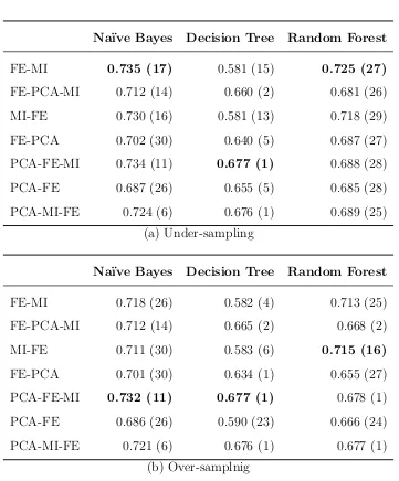
(a) Under-sampling

Na¨ıve Bayes Decision Tree Random Forest

FE-MI 0.718 (26) 0.582 (4) 0.713 (25) FE-PCA-MI 0.712 (14) 0.665 (2) 0.668 (2) MI-FE 0.711 (30) 0.583 (6) 0.715 (16)

FE-PCA 0.701 (30) 0.634 (1) 0.655 (27) PCA-FE-MI 0.732 (11) 0.677 (1) 0.678 (1) PCA-FE 0.686 (26) 0.590 (23) 0.666 (24) PCA-MI-FE 0.721 (6) 0.676 (1) 0.677 (1)

(b) Over-samplnig

0 5 10 15 20 25 30 0.4

0.45 0.5 0.55 0.6 0.65 0.7 0.75

Number of Features

A

UC

FE-MI FE-PCA-MI MI-FE FE-PCA PCA-MI-FE PCA-FE-MI PCA-FE

Figure 5: Carriageway classification with under-sampling AUC values against number of features used in the Na¨ıve Bayes classifier. The performance is highest with features selected by the FE-MI or PCA-FE-MI selection paths.

the peak AUC performances increase in general by a small amount when under-sampling or over-sampling is applied. One effect of performing re-sampling on the data is that the peak AUC performances of the Decision Tree are now achieved with even fewer features in many cases, indicating that the over-fitting problem is intensified.

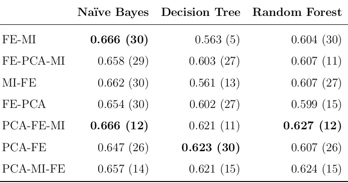
Finally, for the multi-class road type problem we evaluated ECOC, which has shown robustness to imbalance in other domains. Table 6 shows the peak AUC performances for the Weighted-ECOC approach described in (Zhang et al., 2012). For both Na¨ıve Bayes and Random Forest classifiers the results are similar in distribution to when ECOC is not applied, with a small decrease in AUC values in general. The Decision Tree classifier now has a smaller peak AUC performance, but requires more features to achieve it.

6

Discussion

Na¨ıve Bayes Decision Tree Random Forest

FE-MI 0.666 (30) 0.563 (5) 0.604 (30) FE-PCA-MI 0.658 (29) 0.603 (27) 0.607 (11) MI-FE 0.662 (30) 0.561 (13) 0.607 (27) FE-PCA 0.654 (30) 0.602 (27) 0.599 (15) PCA-FE-MI 0.666 (12) 0.621 (11) 0.627 (12)

PCA-FE 0.647 (26) 0.623 (30) 0.607 (26) PCA-MI-FE 0.657 (14) 0.621 (15) 0.624 (15)

Table 6: Peak AUC values when using Weighted-ECOC with the Na¨ıve Bayes, Decision Tree and Random Forest classification algorithms on road type, with the number of features in braces. The highest AUC achieved for each model is highlighted in bold. These results show that Na¨ıve Bayes trained using features produced by PCA-FE-MI will provide the highest performance with fewest features.

using only relevancy. Also, any redundancy analysis should be performed on the signals prior to feature extraction, and followed by a relevancy selection stage. Performing only redundancy feature selection does not provide a good feature ranking in any case, which is likely due to its unsupervised nature.

Also, the choice of methods may change depending on requirements of a system with respect to computing efficiency, rather than just predictive performance. For example, performing selection prior to feature extraction as in MI-FE is much less computationally expensive than selecting from the full feature set, while both methods will provide similar performance with 15 features. We find, however, that features selected using FE-MI or FE-MI provide higher AUC performances with fewer features than MI-FE or PCA-MI-FE. This result may be valuable where there is limit on the feasible number of signals that can be used in a model running on the vehicle’s electronic control unit. In this case, it would also mean that any selection path including PCA is unlikely to be of use, because the principal components produced are a linear combination of all inputs.

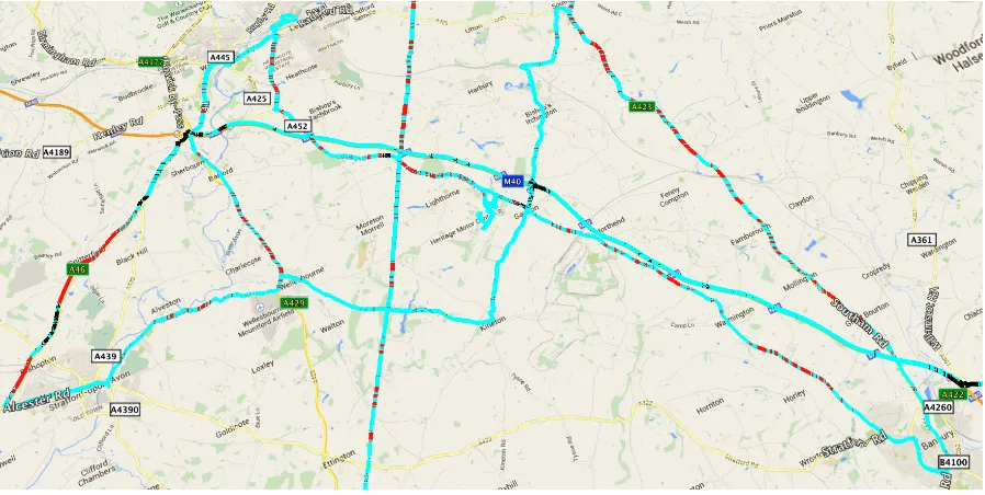
Figure 6: Road map showing correct predictions (Cyan), single roads incorrectly pre-dicted as dual (Red) and dual roads predicted as single (Black) for carriageway classifi-cation. Na¨ıve Bayes classifiers, trained with under-sampled training data and 10 features selected by the PCA-FE-MI selection path are used, with a decision threshold of 0.1. The yellow lines are other roads that are not recorded in our data.

class imbalance in the carriageway classification task, under-sampling or over-sampling the training data increases the AUC performance by a small amount. Although this in-crease in peak AUC performance is also seen in the with the Decision Tree classifier, any signs of over-fitting are exacerbated by under- or over-sampling. Using Weighted-ECOC to mitigate any class imbalance in the road type classification task decreases performance of all models. This may be because the class imbalance in this problem is less severe than in the binary classification task.

Taking into consideration these results, the highest performing model for carriageway classification by AUC is Na¨ıve Bayes, trained with under-sampled data and features selected by FE-MI. This is only a small improvement on the same model built with no under-sampled training data, or with features selected by the PCA-FE-MI selection path. For road classification, the highest performing model is Na¨ıve Bayes, trained with features selected by PCA-FE-MI. This is closely followed by the same model built with features from any of the selection paths containing both a PCA and MI stage.

roads incorrectly labelled as dual roads are red and dual roads incorrectly labelled as

single are black. The predictions were made by 16 Na¨ıve Bayes classifiers, each trained using data from 15 journeys and tested on the remaining one. Data from each journey is used as testing data exactly once and a decision threshold of 0.1 is used to make a prediction for every sample in the dataset. The training data was under-sampled and 10 features selected by the PCA-FE-MI selection path are used in all the models. The image shows a majority predictions are correct, scattered with some short periods of incorrect classifications. These short periods might be labelled correctly if historical classifications are taken into account, such as taking the modal prediction over a temporal window. This, however, would introduce extra delay when the environment changes. The larger red section of road toward the left side of the map is classified incorrectly asdual because it is a straight road with wide lanes and a speed limit of 60mph. The cyan section of road next to this that is incorrectly labelled assingleis actually a road with three lanes, where two are in the direction of travel. These are both examples of edge cases that are sufficiently similar to the other label. It may be possible to detect these cases and act appropriately if the classifier is unable to decide a label with sufficient confidence. One such action may be to assume a default label such as dual and activate a lane departure warning system.

7

Conclusions

In this paper we adapted and applied a data mining methodology to learning driving con-ditions from CAN-bus data, illustrating the approach with the road classification prob-lem. We investigated signal selection, feature extraction and feature selection to produce a successful model for two sub-problems of this domain. Also, as the data collected was imbalanced, techniques to solve this were tested. The data mining methodology was then used to generate models that were capable of accurately predicting the carriageway type or road type using only 2.5 seconds of historical data.

features, meaning that FE-MI or MI-FE may be preferable in deployment. Of these two selection paths, FE-MI provides the best feature set to build a model with. In future, however, we believe that relevancy and redundancy should be considered together (Kohavi and John, 1997). For both carriageway and road classification we found that Na¨ıve Bayes is likely to provide the highest performance, which is improved upon by under-sampling the training data in carriageway classification. The models built for the road classification task were not improved by the Weighted-ECOC technique used to mitigate effects of class imbalance.

In this work the same window length of 2.5 seconds was used in all experiments and for all features, because we found this to be an appropriate size overall (Taylor et al., 2013a). Shorter window lengths caused a decrease in performance, while longer window lengths increased performance minimally and introduced errors shortly after label changes. This may not be the case in general, however, as features extracted using different window lengths capture different information. Two derivative features extracted using short and long windows, for example, would capture short and long term trends in the signal. Further, it may be the case that both of these features should be used in a model for the highest performance.

In this paper, we have considered the problem where location and map data are unavailable at any point (or their use is undesirable). However, if it is possible to obtain a ground truth during driving, even for short periods of time, it may be possible to develop an online learning system for road type classification. If this was the case, affects of concept drift could be investigated (Li et al., 2010). For instance, as a driver becomes more experienced over their lifetime, or tired during a journey, their driving patterns may change with respect to road type. Therefore, it may be essential to update on-line classification models with new information to maintain performance.

References

C.. Antunes and A. Oliveira. Lecture notes in computer science: Temporal data mining: an overview. Proceedings of KDD Workshop on Temporal Data Mining, 2001.

L. Breiman. Random forests. Machine Learning, 45(1):5–32, 2001.

T. Carlson and T. Austin. Development of speed correction cycles. Technical report, Sierra Research, Inc, 04 1997.

Z. Constantinescu, C. Marinoiu, and M. Vladoiu. Driving style analysis using data mining techniques. International Journal of Computers Communications & Control, 5(5):654– 663, 2010.

J. Crossman, H. Guo, Y. Murphey, and J. Cardillo. Automotive signal fault diagnostics -part I: signal fault analysis, signal segmentation, feature extraction and quasi-optimal feature selection. IEEE Transactions on Vehicular Technology, 52(4):1063–1075, july 2003.

S. Escalera, O. Pujol, and P. Radeva. Loss-weighted decoding for error-correcting output coding. International Conference on Computer Vision Theory and Applications, pages 117–122, 2008.

M. Farsi, K. Ratcliff, and M. Barbosa. An overview of controller area network. Computing Control Engineering Journal, 10(3):113–120, 1999.

H. Guo, J. Crossman, Y. Murphey, and M. Coleman. Automotive signal diagnostics using wavelets and machine learning. IEEE Transactions on Vehicular Technology, 49 (5):1650–1662, 2000.

W. Hauptmann, F. Graf, and K. Heesche. Driving environment recognition for adaptive automotive systems. In IEEE International Conference on Fuzzy Systems, volume 1, pages 387–393, 1996.

H. He and E. Garcia. Learning from imbalanced data. IEEE Transactions on Knowledge and Data Engineering, 21(9):1263–1284, 2009.

J. Huang and C. Ling. Using auc and accuracy in evaluating learning algorithms. IEEE Transactions on Knowledge and Data Engineering, 17(3):299–310, 2005.

P. Jansen, W. van der Mark, J. van den Heuvel, and F. Groen. Colour based off-road environment and terrain type classification. InProceedings on IEEE Intelligent Trans-portation Systems, pages 216–221, 2005.

G. John. Enhancements to the data mining process. PhD thesis, stanford university, 1997.

H. Kargupta, R. Bhargava, K. Liu, M. Powers, P. Blair, S. Bushra, J. Dull, K. Sarkar, M. Klein, M. Vasa, and D. Handy. Vedas: A mobile and distributed data stream mining system for real-time vehicle monitoring. InInternational Conference on Data Mining, pages 300–311, 2004.

R. Kohavi and G. John. Wrappers for feature subset selection. Artificial Intelligence, 97 (1-2):273–324, 1997.

R. Langari and J. Won. Intelligent energy management agent for a parallel hybrid vehicle-part I: system architecture and design of the driving situation identification process.

IEEE Transactions on Vehicular Technology, 54(3):925–934, 2005.

P. Li, X. Wu, X. Hu, Q. Liang, and Y. Gao. A random decision tree ensemble for mining concept drifts from noisy data streams. Applied Artificial Intelligence, 24(7):680–710, 2010.

K. Manimala, K. Selvi, and R. Ahila. Optimal feature set and parameter selection for power quality data mining. Applied Artificial Intelligence, 26(3):204–228, 2012.

B. Mehler, B. Reimer, and J. Coughlin. Sensitivity of physiological measures for detecting systematic variations in cognitive demand from a working memory task: An on-road study across three age groups. Human Factors, 54(3):396–412., 2012.

Y. L. Murphey, Zhi Hang Chen, L. Kiliaris, Jungme Park, Ming Kuang, A. Masrur, and A. Phillips. Neural learning of driving environment prediction for vehicle power management. In IEEE International Joint Conference on Neural Networks, pages 3755–3761, 2008.

L. Qiao, M. Sato, and H. Takeda. Learning algorithm of environmental recognition in driving vehicle. IEEE Transactions on Systems, Man and Cybernetics, 25(6):917–925, 1995.

L. Qiao, M. Sato, K. Abe, and H. Takeda. Self-supervised learning algorithm of en-vironment recognition in driving vehicle. IEEE Transactions on Systems, Man and Cybernetics, Part A: Systems and Humans, 26(6):843–850, 1996.

A. Sagheer, N. Tsuruta, R. Taniguchi, and S. Maeda. Appearance feature extraction versus image transform-based approach for visual speech recognition. International Journal of Computational Intelligence and Applications, 6(01):101–122, 2006.

A. Shaikh, D. Kumar, and J. Gubbi. Visual speech recognition using optical flow and support vector machines. International Journal of Computational Intelligence and Applications, 10(02):167–187, 2011.

P. Soda and G. Iannello. Decomposition methods and learning approaches for imbal-anced dataset: An experimental integration. In International Conference on Pattern Recognition, pages 3117–3120, 2010.

I. Tang and T. Breckon. Automatic road environment classification. IEEE Transactions on Intelligent Transportation Systems, 12(2):476–484, 2011.

P. Taylor, F. Adamu-Fika, S. S. Anand, A. Dunoyer, N. Griffiths, and T. Popham. Road type classification through data mining. In Proceedings of the 4th International Con-ference on Automotive User Interfaces and Interactive Vehicular Applications, pages 233–240, 2012.

P. Taylor, N. Griffiths, A. Bhalerao, A. Dunoyer, T. Popham, and Z. Xu. Feature selection in highly redundant signal data: A case study in vehicle telemetry data and driver monitoring. InInternational Workshop Autonomous Intelligent Systems: Multi-Agents and Data Mining, pages 25–36. Springer, 2013a.

R. Wang and S. Lukic. Review of driving conditions prediction and driving style recog-nition based control algorithms for hybrid electric vehicles. InIEEE on Vehicle Power and Propulsion Conference, pages 1–7, 2011.

I. Witten and E. Frank. Data Mining: Practical Machine Learning Tools and Techniques, Third Edition (Morgan Kaufmann Series in Data Management Systems). Morgan Kaufmann, 2005.

M. Wollmer, C. Blaschke, T. Schindl, B. Schuller, B. Farber, S. Mayer, and B. Trefflich. Online driver distraction detection using long short-term memory. IEEE Transactions on Intelligent Transportation Systems, 12(2):273–324, 2011.

X. Zhang, J. Wu, Z. Chen, and P. Lv. Optimized weighted decoding for error-correcting output codes. InIEEE International Conference on Acoustics, Speech and Signal Pro-cessing, pages 2101–2104, 2012.