warwick.ac.uk/lib-publications
Original citation:
Tindale, Elizabeth and Chapman, Sandra C.. (2016) Solar cycle variation of the statistical
distribution of the solar windεparameter and its constituent variables. Geophysical Research
Letters, 43.
http://dx.doi.org/10.1002/2016GL068920
Permanent WRAP URL:
http://wrap.warwick.ac.uk/79529
Copyright and reuse:
The Warwick Research Archive Portal (WRAP) makes this work of researchers of the
University of Warwick available open access under the following conditions.
This article is made available under the Creative Commons Attribution 4.0 International
license (CC BY 4.0) and may be reused according to the conditions of the license. For more
details see:
http://creativecommons.org/licenses/by/4.0/
A note on versions:
The version presented in WRAP is the published version, or, version of record, and may be
cited as it appears here.
Solar cycle variation of the statistical distribution of the solar
wind
𝜖
parameter and its constituent variables
E. Tindale1and S. C. Chapman1
1CFSA, Physics Department, University of Warwick, Warwick, UK
Abstract
We use 20 years of Wind solar wind observations to investigate the solar cycle variation of the solar wind driving of the magnetosphere. For the first time, we use generalized quantile-quantile plots to compare the statistical distribution of four commonly used solar wind coupling parameters, Poynting flux,B2, the𝜖parameter, andvB, between the maxima and minima of solar cycles 23 and 24. We find thedistribution is multicomponent and has the same functional form at all solar cycle phases; the change in distribution is captured by a simple transformation of variables for each component. The𝜖parameter is less sensitive than its constituent variables to changes in the distribution of extreme values between successive solar maxima. The quiet minimum of cycle 23 manifests only in lower extreme values, while cycle 24 was less active across the full distribution range.
1. Introduction
The 11 year solar cycle is variable, with an extended minimum observed in cycle 23 and a notably quiet max-imum in the most recent cycle 24 [Lockwood, 2013;Zerbo and Richardson, 2015]. Satellites in the solar wind upstream of Earth provide a comprehensive data set covering several solar cycles. Variables observed in situ are combined into solar wind parameters that aim to capture the driving of the magnetosphere by the solar wind [e.g.,Gonzales, 1990]. This letter focuses on the systematic changes in the statistical distributions of these solar wind parameters between different phases of the solar cycle.
The Poynting fluxSis the energy flux density carried by the electromagnetic fields of the solar wind plasma. Along withS, we will consider three of the most commonly used parameters: the𝜖parameter [Perreault and Akasofu, 1978], in whichSis scaled to account for energy transport into the magnetosphere [Koskinen and Tanskanen, 2002]; the westward electric field, estimated asvxBz[Burton et al., 1975]; and finally,B2, found to
be more closely related to solar activity [Kiyani et al., 2007].
There has been extensive work on the statistics of solar wind variables. Early work [Burlaga and King, 1979] identified an approximately lognormal probability density function (PDF) of the magnetic field strength. Feynman and Ruzmaikin[1994] showed that the PDF of the interplanetary magnetic field (IMF) field strength could not be exactly lognormal due to nonzero kurtosis, which was substantiated later byBurlaga and Ness [1996] who determined the PDF to be lognormal with an exponential tail but also discussed the possibility of a Pareto tail.Koons[2001] successfully fitted the Gumbel class of extreme value distribution to annual maxima of the 60 MeV proton flux.Moloney and Davidsen[2010] found that the block maxima of the𝜖 param-eter follow the Fréchet distribution; however, this fit overestimated the highest values. Since the Fréchet class is the limiting distribution for a variable that has a PDF with a power law tail [Schumann et al., 2012], a Fréchet fit to block maxima of the𝜖parameter would support Burlaga’s earlier proposal of a lognormal PDF with a Pareto tail.Burlaga and Lazarus[2000] also found evidence for lognormal distributions of the solar wind speed, density, and temperature, and that these distributions vary with the phase of the cycle. They attributed this variation to the dominance of corotating streams in the solar wind at solar minimum [Tsurutani et al., 2006]. Common to all these findings is the multicomponent nature of PDFs of solar wind variables.
A complementary approach to the statistical analysis of solar wind variables is the use of bursts. These are defined as the integrated signal over periods where the variable continuously exceeds a given threshold; they have been used to compare the solar wind with both solar flares [Moloney and Davidsen, 2011] and geomag-netic indices [Freeman et al., 2000a]. The PDFs of burst lifetimes of𝜖,(vxBz)s,B2, andShave all been found
RESEARCH LETTER
10.1002/2016GL068920
Key Points:
• Solar wind parameter statistics change with solar cycle phase while preserving PDF functional form • Solar wind𝜖changes in a manner
distinct from other coupling parameters
• Results are independent of PDF functional form
Supporting Information: • Figure S1
• Figure S2 • Figure S3
• Supporting Information S1
Correspondence to: E. Tindale,
Citation:
Tindale, E., and S. C. Chapman (2016), Solar cycle variation of the statistical distribution of the solar wind𝜖parameter and its constituent variables,Geophys. Res. Lett.,
43, doi:10.1002/2016GL068920.
Received 30 MAR 2016 Accepted 12 MAY 2016
Accepted article online 17 MAY 2016
©2016. The Authors.
Geophysical Research Letters
10.1002/2016GL068920
to be power law with an exponential roll off [Wanliss and Weygand, 2007;Freeman et al., 2000b], as has the distribution of waiting times of bursts inBz,S[D’Amicis et al., 2006]. Of these fits,Wanliss and Weygand[2007] found the power law exponents of the𝜖and(vxBz)sdistributions to be solar cycle dependent; however, when looking at higher thresholds,Moloney and Davidsen[2014] found no such dependency. In the related studies of geomagnetic indices,Freeman et al.[2000a] found the distribution of burst lifetimes ofAUandALto be multicomponent, including a power law and exponential cutoff similar to𝜖, andHush et al.[2015] found a multicomponent distribution ofAEburst size, including a solar cycle-dependent exponential component at extreme values.
While these studies have been successful in fitting parts of the distribution of solar wind parameters, there are still open questions, including how the PDF changes over the solar cycle and which of the constituent variables within a parameter such as𝜖drives these changes. In this paper, we address these questions, with the first application of quantile-quantile (QQ) plots [Gilchrist, 2000] to the comparison of observed distributions of each solar wind parameter measured at different phases of the solar cycle. We examine the changes in the cumulative distribution functions (CDFs) of the coupling parametersS,B2,𝜖, and(v
xBz)sin cycles 23 and
24, between each maximum and minimum, between successive maxima, and between successive minima. In each case the distribution is multicomponent, and we find that over a broad range each subcomponent has a functional form that remains unchanged across all phases of the solar cycle. The change in CDF, and hence PDF, is captured by a transformation of variables for each subcomponent; this transformation takes the form ofP(x)→P(𝛼x+𝛽), independent of the underlying PDF functional form. Our results quantify the effect of the quiet minimum of solar cycle 23 and the quiet maximum of cycle 24 on the likelihood of observed values of these parameters. We see systematic changes in the PDFs of the constituent variables of𝜖and identify which variable drives the variation in the statistics of𝜖. We find that the statistics of𝜖can be less sensitive to these changes than those of its constituent variables.
In section 2 we introduce the data set and solar wind parameters. In section 3 we describe the QQ plot method and apply it to the solar wind Poynting flux. In section 4 we repeat this analysis for parametersB2, solar wind
𝜖,BzandvxBz, and for all parameters across the full solar cycles. We conclude in section 5.
2. Data
Data from the Magnetic Fields Investigation and Solar Wind Experiment on the Wind spacecraft were pro-vided by National Aeronautics and Space Administration/Goddard Space Flight Center (NASA/GSFC’s) OMNI data set. Data were only taken at those times when the spacecraft was situated in the upstream solar wind. During preprocessing, the 15 s cadence interplanetary magnetic field (IMF) and 92 s ion plasma velocity are interpolated to 1 min resolution. The plasma velocity measurements include both fast and slow streams, and all measurements are in geocentric solar magnetospheric (GSM) coordinates. One year of data was taken spanning each of the minima and maxima of cycle 23 and cycle 24, using inclusive dates December 1995 to November 1996 (cycle 23 minimum), October 1999 to September 2000 (cycle 23 maximum), August 2007 to July 2008 (cycle 24 minimum), and November 2013 to October 2014 (cycle 24 maximum). Data gaps are reasonably evenly distributed between successive maxima and minima; they typically cover∼10% of the data, ranging from∼5% for the minimum of solar cycle 24 to∼26% for the maximum of cycle 23. The remaining sample sizes are of order 400,000 samples in each data set. The Wind satellite orbitsL1 and is, for our yearlong samples at maxima and minima, within 100REof the Sun-Earth line. It is outside this range for∼8% of the full data set.
The Poynting flux,S, is the characteristic energy flux carried by the solar wind. For ideal magnetohydrody-namics, the electric field isE= −v×B, so that the component of Poynting flux along the Sun-Earth line is approximated by
S= − 1 𝜇0
vx
(
B2
y+B
2
z
)
. (1)
The𝜖parameter is based on the Poynting flux but is scaled to account for the interaction between the solar wind and magnetosphere. In SI units it is
𝜖=4𝜋 𝜇0
vB2
Ssin
4(𝜃
2 )
l2
wherevis the ion plasma speed,BSis the magnitude of the IMF with southwardBz,l0is a length scale taken to be 7RE, and𝜃=tan−1(B
y∕Bz)is the clock angle. The𝜖parameter depends on all three components of the
IMF, while the Poynting flux depends onByandBzonly.
Energy transfer between solar wind and the magnetosphere is in part ordered by the flux of southward directed IMF (i.e., negativeBZin GSM), due to the increased rate of magnetospheric reconnection. We there-fore calculate the solar wind parametersSandB2for both the full data set and the subset of data whereB
Z<0
and the magnetosphere coupling parameters𝜖andvxBzat times of southward IMF only. After removing the
northward IMF values, the southward IMF subsets of data contained approximately 200,000 data points. The subscriptSwill denote the southward IMF only subsets of each parameter.
3. QQ Plots for Poynting Flux
The quantile-quantile (QQ) plot is a tool for comparing two statistical distributions. The distribution of an independently and identically (iid) random variableXcan be described both by its probability density function (PDF),P(x), and the corresponding cumulative density function (CDF),C(x), which are related via
P(x) = dC(x)
dx (3)
so thatC(x)is the likelihood that the value of variableXwill occur below a valuex(X≤x). The CDF can be inverted, so that for any likelihoodq, a valuex(q)can be calculated such that the likelihood of a measurement ofXoccurring belowx(q)isq. The valuex(q)is referred to as theqth quantile of the distribution of variableX; for example, theq=0.5quantile of the distribution,x(0.5), is the median: the value below which 50% of the data lie.
Consider two iid random variables,X1andX2, distributed according to PDFsP1(x1)andP2(x2)with
correspond-ing CDFsC1(x1)andC2(x2). The quantiles of the two distributions are as follows:
x1(q1) =C−1 1 (q1)
x2(q2) =C2−1(q2)
(4)
whereC−1(q)is the inverse of CDFC(x(q)). The QQ plot then has as its coordinates the quantilesx 1(q)and
x2(q), where the likelihoodqis a parametric coordinate. IfX1andX2have same distribution, their quantiles
will be the same, and so a straight “y=x” line of gradient 1 will be recovered. Any other straight line on the QQ plot would be described by
x2(q) =𝛼x1(q) +𝛽, (5)
in which case the CDFs are related by a transformation of variables:
C2(x) =C1
(
x−𝛽 𝛼
)
. (6)
With equation (3) this yields
P2(x) =
1
𝛼P1
(
x−𝛽 𝛼
)
, (7)
so that the corresponding PDFs are related by the same transformation of variables. The scaling parameter𝛼 preserves the normalization, so that the integrated PDF is unity. Hence, if the QQ plot is linear, the functional form of the underlying PDF of both variablesX1andX2is the same, subject to a transformation of variables fromxto(x−𝛽)∕𝛼. The parameter𝛼denotes a change in scale, while𝛽is a shift in location. A positive𝛽value indicates an increase in mean, so that the likelihood of large values ofXincreases as the whole PDF is shifted. If𝛼 >1, a given likelihoodqcorresponds to a larger value ofX, resulting in the stretching of the PDF tail. This in turn modifies the raw higher moments of the distribution; however, the standard measures of skewness and kurtosis can be normalized to account for the change in scale [Gilchrist, 2000]. Both𝛼and𝛽can be found from the data with a linear regression to the QQ plot.
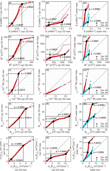
Figure 1 shows QQ plots comparing the distributions of Poynting flux,B2,𝜖andvBbetween solar cycle phases;
Geophysical Research Letters
10.1002/2016GL068920
Figure 1.QQ plots for (ai–aiii) solar wind Poynting flux, (bi–biii)B2, (ci–ciii) the𝜖
the successive maxima, and in the right column we compare each cycle’s maximum to its minimum. In each case we compare the 0.0001 to 0.9999 quantiles. A plot in the same format is given for additional quantities in the supporting information, along with a discussion of uncertainties.
Figures 1ai–1aiii show the results for the solar wind Poynting flux. In each case the QQ plots are multicom-ponent, with three approximately linear regions. A linear region of the QQ plot indicates that the functional form of the PDF in that region does not change; thus, a transformation of variables captures how the distribution is changing over the solar cycle, as described above. These ranges are indicated on the plots. We perform a three-component linear-piecewise fit to these plots. TheR2statistic associated with the each linear
fit (given in Tables S1–S3 in the supporting information) exceeds 0.9 in almost all cases, indicating that the linear transformations provide a good representation of the change in distribution.
The QQ plot of Poynting flux with southward IMF,SS, comparing successive minima (Figure 1ai) consists of
three such approximately linear regions: a “bulk component,” containing data in the 0 to 0.9637 quantiles; a “high component” spanning the 0.9637 to 0.9993 quantiles; and an “extreme component,” which includes values above the 0.9993 quantile. The bulk component has an𝛼value of 0.864(2), where the error denotes the 95% confidence interval of the value, and a𝛽close to zero. This component of the distribution thus shows a small change in scale between the two minima, so that its PDF essentially does not change. The high com-ponent has a significant change in scale of𝛼=1.90(3), as well as a shift in location of𝛽=−0.0237(11). Finally, the extreme component undergoes a transformation ofSS,24=0.197(45)SS,23+0.118(5), showing a decrease
in the scale of these values, but a large (∼10%) increase in their mean. The high and extreme components appear above they= xreference line, so that the increased activity of the minimum of cycle 24 relative to cycle 23 is manifest mainly in these extreme values, rather than in the bulk of the distribution.
Conversely, we can see that in Figure 1aii the quantiles all lie below they=xline, so that the maximum of cycle 24 was significantly less active than the maximum of cycle 23. Again, the QQ plot can be divided into linear regions which we denote as bulk, high, and extreme components. These linear relationships again indicate that within each of the components of the underlying PDF, the functional form is the same at both solar maxima. The crossover points between these regions of the CDF occur atq= 0.9800 andq=0.9988. Unlike the change between successive minima, the bulk component of the distribution changes scale significantly between the successive maxima, with𝛼=0.545(1). The location of the bulk component does not change. The transformation of variables for the high component wasSS,24=0.209(2)SS,23+0.0231(4)and for the extreme component wasSS,24=1.32(20)SS,23−0.409(88). The high component of the PDF therefore decreases in scale but slightly increases in mean, while the opposite is true for the extreme component. We repeated this analysis comparing the full 11 year data sets of cycles 23 and 24 (see supporting information) and find that cycle 23 is overall more active.
Between the successive maxima, the translations of the high and extreme components are sensitive to whether the full data set or the southward IMF subset is included in the CDF. The bulk component undergoes approximately the same transformation of variables in both cases. The change of scale𝛼of the high compo-nent increases from𝛼 =0.209(2)forSSto𝛼= 0.366(5), while for the extreme component𝛼is roughly the
same, changing from𝛼=1.32(20)to𝛼=1.42(10). The shift in location𝛽is∼50% smaller for the high compo-nent and∼20% larger for the extreme component, once the northward IMF values ofSare included. The QQ plot thus has three well-defined linear components that translate according to equation (5) between phases of the solar cycle, irrespective of whether or not northward IMF values are included. However, the changes in scale and location (𝛼and𝛽) of the underlying PDF are more pronounced if we only consider the southward IMF subset.
Geophysical Research Letters
10.1002/2016GL068920
scale𝛼 = 5.90±1.98and large shift in location𝛽 = −0.618(266). Therefore, the quietness of cycle 24 is manifest in the bulk and high components, which are the same at maximum and minimum; only the extreme values above theq=0.9989quantile show increased likelihood at maximum relative to the cycle minimum.
4. QQ Plots for
B
2,
𝝐
S
,
B
z,S, and
(
v
xB
z)
SFigures 1bi–1biii through 1ei–1eiii plot the above solar cycle phase comparisons for theB2,B
z,S,𝜖S, and(vxBz)S
parameters, with the latter three calculated using only values with southward IMF. The QQ plots can again be split into multiple approximately linear components, withR2values consistently above 0.9, so that the PDF
functional form is approximately invariant for all parameters; it, again, simply translates as in equation (5).
Quantiles of both the full and southward IMF onlyB2data sets are shown in Figures 1bi–1biii. Qualitatively,
these panels show the same behavior as in Figures 1ai–1aiii, indicating thatSsimply tracksB2. In all three
plots, the transitions between components occur at similar quantiles for bothB2
SandSS. However, although
the trends are the same, the𝛼and𝛽parameters differ betweenSSandB2, suggesting that the solar wind speed
does not affect the form of the transformations but does alter the details. The comparison of the solar maxima (Figure 1bii) also shows the same sensitivity as the Poynting flux to whether all values or the southward IMF only subset is used.
Between successive solar minima, the QQ plot for𝜖S(Figure 1ci) is qualitatively similar to those ofSSandB2S
(Figures 1ai and 1bi). However, when we consider how the distribution translates between successive solar maxima (Figure 1cii) the distribution of the𝜖Sparameter transforms in a remarkably different way to the other variables. The PDF retains its functional form and is translated by a single change in scale over the full range. The𝛼value of this transformation is 0.501(1), which is similar to the𝛼values of the bulk components of the SSandB2
S. The high and extreme values of𝜖S thus do not retain the distinct changes between successive
maxima seen inSSandB2
S. Similar behavior of𝜖Sis found when comparing the maximum and minimum of
cycle 23 in Figure 1ciii; that is, the high and extreme components are indistinguishable and translate with a single change of scale𝛼=4.81(9). Now,𝜖depends upon all three components of magnetic field, whereas the Poynting flux depends on theyandzcomponents only;𝜖also includes a factor that depends on the clock angle. In Figure S1, we plot, in the same format as Figure 1, the changes inB2
xandB2yz=B2y+B2z, along with the
clock angle contribution to𝜖. We see that the distribution of the clock angle contribution does not change between the different phases of the solar cycles; therefore, this does not explain the relative insensitivity of𝜖. However, the distributions ofB2
xandB2yztranslate in opposite directions on the plot; for example, the extreme
components have𝛼 <1and𝛼 >1, respectively (values are𝛼=0.0602(408)and𝛼=1.50(20)). When these are combined within a single parameter, they may tend to suppress these changes. We have repeated this analysis (see supporting information) for the Milan and Newell coupling parameters [Milan et al., 2008;Newell et al., 2007] and find that they are intermediate in sensitivity between𝜖and Poynting flux. In common with the Poynting flux, they only depend on theyandzcomponents of the IMF.
Within Figures 1di–1diii and 1ei–1eiii, the distributions of variables Bz,S and(vxBz)S show little change between the two minima except at the extreme values (Figures 1di and 1ei), with less sharp transitions between components. The comparison of the maxima for these variables (Figures 1dii and 1eii) shows three linear components, but again with less clear transitions; this is reflected in the lowerR2values, which are
0.9722 and 0.9670 for the high component ofBz,Sand(vxBz)S, respectively, compared to 0.9938 and 0.9829
forSSandB2S. The similarity of the QQ plots forBz,Sand(vxBz)Sagain suggests that the magnetic field drives
the variation of the distribution of the constructed parameters. The solar wind speed also contributes to the change in distribution between the maximum and minimum of cycle 24: compare Figures 1diii and 1eiii with Figure S1aiii in the supporting information.
In Figures 1aiii, 1biii, and 1ciii we see similar qualitative behavior across the parameters. The bulk and high components of the cycle 24 QQ plot are close to they = xline in most cases, indicating that the distribu-tion of each variable for cycle 24 was the same at maximum and minimum up to the highest quantiles. The outstanding case is in Figure 1diii, where the bulk component of theBz,Sdistribution transforms in the same manner for both cycle 23 and 24, up to theq=0.9800. The relatively low activity of cycle 24 is also evident; for all variables, the quantiles of cycle 24 lie below those of cycle 23. The extreme component occurs between q= 0.9989andq=0.9995for all variables in cycle 24, and all except𝜖Sand(vxBz)Sin cycle 23, suggesting
Finally, we compared the distributions of the two full cycles; see the supporting information for QQ plots and a detailed discussion. Overall, cycle 23 shows higher activity, despite its quiet minimum. For all four parameters, ranges are again found over which the QQ plots are linear, suggesting that the transformation of variables in equation (5) captures the change in the PDF.
5. Summary
We investigated how the probability density functions of four solar wind-magnetosphere coupling parame-ters change over the two most recent solar cycles using quantile-quantile plots. The distributions for Poynting flux,B2,𝜖Sand the westward electric field(v
xBz)Swere compared between cycle 23 minimum and cycle 24
minimum, between cycle 23 maximum and cycle 24 maximum, and between the maximum and minimum of each of cycles 23 and 24.
We found that for all parameters the PDF has a multicomponent functional form which does not change over the solar cycle or between cycles. Instead, a linear transformation of variables for each component is required to map that region of the PDF from one solar cycle phase to another. These transformations can be found by fitting least squares regressions to linear regions of the QQ plot. We identified three regions of the distributions in the QQ plots; the bulk component, up toq∼0.96, and beyond this the high and extreme components. The bulk component undergoes a change in scale between solar maxima but is roughly the same at both minima. The high and extreme components forS,B2and(v
xBz)Sare each associated with a unique change in both
scale and location. The𝜖Sparameter behaves differently toSS,B2
Sand(vxBz)Sas the change in its PDF between
successive maxima is captured by a single change in scale over the full range, so the high and extreme values are insensitive to the changes in their distribution seen inSSandB2
S.
The QQ plots forSresemble those ofB2, and likewise the QQ plots for(v
xBz)Strack those ofBz,S, implying that
changes inBdrive changes in the PDFs of the solar wind coupling parameters. Cycle 23 exhibited a quieter minimum than cycle 24, which is manifest in the distribution as larger amplitude (quantile) high and extreme components at the minimum of cycle 24 than cycle 23, while the bulk component was roughly the same for both minima. The overall activity of cycle 23 was higher than that of cycle 24, seen across the distribution at the maximum of cycle 23 compared to the maximum of cycle 24. The changes in the distribution ofSandB2
between successive maxima were also found to be more pronounced in the distribution of values when IMF is southward.
As the functional form of the distribution of each solar wind variable does not change between extrema of cycles 23 and 24, it could be an intrinsic property, and as such would remain the same in future cycles. This qualitative property of the full distribution provides a benchmark for models and may support prediction of the likelihood of extreme space weather events. However, as we have shown, this depends on the variable chosen, as the𝜖parameter is less sensitive to changes in the likelihood of its large values than theS,B2and
(vxBz)Svariables.
References
Burlaga, L. F., and J. H. King (1979), Intense interplanetary magnetic fields observed by geocentric spacecraft during 1969-1975,J. Geophys. Res.,84(A11), 6633–6640, doi:10.1029/JA084iA11p06633.
Burlaga, L. F., and A. J. Lazarus (2000), Lognormal distributions and spectra of solar wind plasma fluctuations: Wind 1995–1998,J. Geophys. Res.,105(A2), 2357–2364, doi:10.1029/1999JA900442.
Burlaga, L. F., and N. F. Ness (1996), Magnetic fields in the distant heliosphere approaching solar minimum: Voyager 1 and 2 observations during 1994,J. Geophys. Res.,101(A6), 13,473–13,481, doi:10.1029/96JA00523.
Burton, R. K., R. L. McPherron, and C. T. Russell (1975), An empirical relationship between interplanetary conditions andDst,J. Geophys. Res.,
80(31), 4204–4214, doi:10.1029/JA080i031p04204.
D’Amicis, R., R. Bruno, B. Bavassano, V. Carbone, and L. Sorriso-Valvo (2006), On the scaling of waiting-time distributions of the negative IMF
Bzcomponent,Ann. Geophys.,24, 2735–2741, doi:10.5194/angeo-24-2735-2006.
Feynman, J., and A. Ruzmaikin (1994), Distributions of the interplanetary magnetic field revisited,J. Geophys Res.,99(A9), 17,645–17,651, doi:10.1029/94JA01098.
Freeman, M. P., N. W. Watkins, and D. J. Riley (2000a), Evidence for a solar wind origin of the power law burst lifetime distribution of the
AEindices,Geophys. Res. Lett.,27(8), 1087–1090, doi:10.1029/1999GL010742.
Freeman, M. P., N. W. Watkins, and D. J. Riley (2000b), Power law distributions of burst duration and interburst interval in the solar wind: Turbulence or dissipative self-organized criticality?,Phys. Rev. E,62(6), 8794–8797, doi:10.1103/PhysRevE.62.8794.
Gilchrist, W. G. (2000),Statistical Modelling With Quantile Functions, Chapman and Hall, Fla.
Gonzales, W. D. (1990), A unified view of solar wind-magnetosphere coupling functions,Planet. Space. Sci.,38(5), 627–632, doi:10.1016/0032-0633(90)90068-2.
Hush, P., S. C. Chapman, M. W. Dunlop, and N. W. Watkins (2015), Robust statistical properties of the size of large burst events inAE,
Geophys. Res. Lett.,42, 9197–9202, doi:10.1002/2015GL066277. Acknowledgments
Geophysical Research Letters
10.1002/2016GL068920
Kiyani, K., S. C. Chapman, B. Hnat, and R. M. Nicol (2007), Self-similar signature of the active solar corona within the inertial range of solar-wind turbulence,Phys. Rev. Lett.,98, 211101, doi:10.1103/PhysRevLett.98.211101.
Koons, H. C. (2001), Statistical analysis of extreme values in space science,J. Geophys. Res.,106(A6), 10,915–10,921, doi:10.1029/2000JA000234.
Koskinen, H. E., and E. I. Tanskanen (2002), Magnetospheric energy budget and the epsilon parameter,J. Geophys. Res.,107(A11), 1415, doi:10.1029/2002JA009283.
Lockwood, M. (2013), Reconstruction and prediction of variations in the open solar magnetic flux and interplanetary conditions,Living Rev. Sol. Phys.,10, 4. [Available at http://www.livingreviews.org/lrsp-2014-4, (accessed 16/02/16).]
Milan, S. E., P. D. Boakes, and B. Hubert (2008), Response of the expanding/contracting polar cap to weak and strong solar wind driving: Implications for substorm onset,J. Geophys. Res.,113, A09215, doi:10.1029/2008JA013340.
Moloney, N. R., and J. Davidsen (2010), Extreme value statistics in the solar wind: An application to correlated Levy processes,J. Geophys Res.,115, A10114, doi:10.1029/2009JA015114.
Moloney, N. R., and J. Davidsen (2011), Extreme bursts in the solar wind,Geophys. Res. Lett.,38, L14111, doi:10.1029/2011GL048245. Moloney, N. R., and J. Davidsen (2014), Stationarity of extreme bursts in the solar wind,Phys. Rev. E,89, 052812,
doi:10.1103/PhysRevE.89.052812.
Newell, P. T., T. Sotirelis, K. Liou, C.-I. Meng, and F. J. Rich (2007), A nearly universal solar wind-magnetosphere coupling function inferred from 10 magnetospheric state variables,J. Geophys. Res.,112, A01206, doi:10.1029/2006JA012015.
Perreault, P., and S.-I. Akasofu (1978), A study of geomagnetic storms,Geophys. J. R. Astron. Soc.,54(3), 547–573, doi:10.1111/j.1365-246X.1978.tb05494.x.
Schumann, A. Y., N. R. Moloney, and J. Davidsen (2012), Extreme value and record statistics in heavy-tailed processes with long-range memory, inExtreme Events and Natural Hazards: The Complexity Perspective, edited by A. S. Sharma, AGU, Washington, D. C., doi:10.1029/2011GM001088.
Tsurutani, B. T., et al. (2006), Corotating solar wind streams and recurrent geomagnetic activity: A review,J. Geophys Res.,111, A07S01, doi:10.1029/2005JA011273.
Wanliss, J. A., and J. M. Weygand (2007), Power law burst lifetime distribution of theSYM-Hindex,Geophys. Rev. Lett.,34, L04107, doi:10.1029/2006GL028235.
Zerbo, J.-L., and J. D. Richardson (2015), The solar wind during current and past solar minima and maxima,J. Geophys. Res. Space Physics,
![Rheumatoid Arthritis of the Temporomandibular Joint; Comparison of Digital Panoramic Radiographs Taken Using the Joint Limitation Program [JLA View] and CT Scans](data:image/gif;base64,R0lGODlhAQABAIAAAP///wAAACH5BAEAAAAALAAAAAABAAEAAAICRAEAOw==)