warwick.ac.uk/lib-publications
Original citation:
Treviño, Santiago, Nyberg, Amy, Del Genio, Charo I. and Bassler, Kevin E.. (2015) Fast and
accurate determination of modularity and its effect size. Journal of Statistical Mechanics :
Theory and Experiment, 2015 (2). P02003.
Permanent WRAP URL:
http://wrap.warwick.ac.uk/83933
Copyright and reuse:
The Warwick Research Archive Portal (WRAP) makes this work by researchers of the
University of Warwick available open access under the following conditions. Copyright ©
and all moral rights to the version of the paper presented here belong to the individual
author(s) and/or other copyright owners. To the extent reasonable and practicable the
material made available in WRAP has been checked for eligibility before being made
available.
Copies of full items can be used for personal research or study, educational, or not-for-profit
purposes without prior permission or charge. Provided that the authors, title and full
bibliographic details are credited, a hyperlink and/or URL is given for the original metadata
page and the content is not changed in any way.
Publisher’s statement:
“This is an author-created, un-copyedited version of an article accepted for publication in
Journal of Statistical Mechanics : Theory and Experiment The publisher is not responsible for
any errors or omissions in this version of the manuscript or any version derived from it. The
Version of Record is available online at
http://dx.doi.org/10.1088/1742-5468/2015/02/P02003
”
A note on versions:
The version presented here may differ from the published version or, version of record, if
you wish to cite this item you are advised to consult the publisher’s version. Please see the
‘permanent WRAP URL’ above for details on accessing the published version and note that
access may require a subscription.
arXiv:1412.8669v1 [physics.soc-ph] 29 Dec 2014
its effect size
Santiago Treviño III1,2, Amy Nyberg1,2, Charo I. Del Genio3,4,5,6 and Kevin E. Bassler1,2,6
1Department of Physics, 617 Science & Research 1, University of Houston, Houston, Texas 77204-5005, USA
2Texas Center for Superconductivity, 202 Houston Science Center, University of Houston, Houston, Texas 77204-5002, USA
3Warwick Mathematics Institute, University of Warwick, Gibbet Hill Road, Coventry CV4 7AL, United Kingdom
4Centre for Complexity Science, University of Warwick, Gibbet Hill Road, Coventry CV4 7AL, United Kingdom
5Warwick Infectious Disease Epidemiology Research (WIDER) Centre, University of Warwick, Gibbet Hill Road, Coventry CV4 7AL, United Kingdom 6Max Planck Institute for the Physics of Complex Systems, Nöthnitzer Str. 38, D-01187 Dresden, Germany
E-mail: [email protected]
1. Introduction
Networked systems, in which the elements of a set of nodes are linked in pairs if they share a common property, often feature complex structures extending across several length scales. At the lowest length scale, the number of links of a node defines its degreek. At the immediately higher level, the links amongst the neighbours of a node define the structure of a local neighbourhood. The nodes in some local neighbourhoods can be more densely linked amongst themselves than they are with nodes belonging to other neighbourhoods. In this case, we refer to these densely connected modules as communities. A commonly used indicator of the prominence of community structure in a complex network is its maximum modularity Q. Given a partition of the nodes into modules, the modularity measures the difference between its intra-community connection density and that of a random graph null model [1, 2, 3, 4]. Highly modular structures have been found in systems of diverse nature, including the World Wide Web, the Internet, social networks, food webs, biological networks, sexual contacts networks, and social network formation games [5, 6, 7, 8, 9, 10, 11, 12, 13, 14]. In all these real-world systems, the communities correspond to actual functional units. For instance, communities in the WWW consist of web pages with related topics, while communities in metabolic networks relate to pathways and cycles [7, 12, 15, 16]. A modular structure can also influence the dynamical processes supported by a network, affecting synchronization behaviour, percolation properties and the spreading of epidemics [17, 18, 19]. The development of methods to detect the community structure of complex systems is thus a central topic to understand the physics of complex networks [20, 21, 22, 23, 24].
Figure 1. Different partitions of the same network. The partition on the left divides the network into two communities with densely connected nodes. The partition on the right divides the same network into modules consisting of disconnected nodes, resulting in a low value of the modularity.
degree of 1 or more. A quantitative comparison ofz-scores can be used to complement that of the modularities of different networks, including those with different numbers of nodes and/or links.
2. Modularity and effect size
Given a network with N nodes andm links, one can define a partition of the nodes by grouping them into communities. Letciindicate the community to which nodeiis assigned, and let{c}be the set of communities into which the network was partitioned. Then, the modularityqof the partition is
q{c}=
1 2m
X
ij
Aij−
kikj 2m
δci,cj, (1)
whereki is the degree of nodei, andA is the adjacency matrix, whose(i, j)element is 1 if nodesiandjare linked, and 0 otherwise. With this definition, the value ofqis larger for partitions where the number of links within communities is larger than what would be expected based on the degrees of the nodes involved [29]. Of course, even in the case of a network with quite a well-defined community structure, it is usually possible to define a partition with a small modularity. For instance, one can artificially split the network into modules consisting of pairs of unconnected nodes taken from different actual communities (see Fig. 1). Thus, in order to properly characterize the community structure it is instead necessary to find the particular partition{C}that maximizes the modularity,
{C}= arg max
{c}
q{c} .
Henceforth, we indicate withQ the maximum modularity of a network, which is the modularity of the partition{C}:
Q=q{C}= max
{c}
q{c} = max
{c}
1 2m
X
ij
Aij−kikj 2m
δci,cj
.
The maximum modularity Qcorresponds to the particular partition of the network that divides it into the most tightly bound communities. However, simply finding this partition is not sufficient to determine the statistical importance of the community structure found.
To see this, consider an ensemble of random graphs with a fixed number of nodes
that they have no real communities. Then, one could assume a vanishing average modularityhqi{c} on the ensemble. However, the amount of community structure is
quantified by the extremal measureQ, rather than hqi{c}. Thus, one cannot exclude
a priori the existence of a partition with non-zero modularity even on a completely random graph. This implies that one can attach a fuller meaning to the maximum modularity of a given network by comparing it to the expected maximum modularity of an appropriate set of random graphs. Then, the comparison defines an effect size for the modularity, measuring the statistical significance of a certain observed Q. Of course, the random graph ensemble must be appropriately chosen to represent a randomized version of the network analyzed.
A suitable random graph set for this study is given by the Erdős-Rényi (ER) modelG(N, p)[30]. In the model, links between any pair of nodes exist independently with fixed probability p. As there is no other constraint imposed, ER graphs are completely random, which makes them a natural choice for a null model. Of course, it is conceivable that another null model could be used for specific types of networks. In this case, one could generate random ensembles of networks with a specified set of constraints, using appropriate methods such as degree-based graph construction [31, 32]. To find the correct probability to use, we require that the expected number of links in each individual graph must equal the number of links in the network we are studying. The expected number of links in an Erdős-Rényi network withN nodes is
hmi= pN(N−1)
2 .
Thus, the probability of connection must be
p= 2m
N(N−1). (2)
Then, we can compareQ with the expected maximum modularityhQERiof the ER ensemble thus defined. One simple way to perform the comparison is calculating the difference between Q and hQERi. However, while this approach provides a certain estimate of the importance of Q, it is not entirely satisfactory. In fact, the same difference acquires more or less significance depending on the width of the distribution ofhQERi. Then, it is a natural choice to normalize the difference between maximum modularities dividing it by the standard deviationσER ofhQERi
z= Q− hQERi
σER
. (3)
The equation above defines a particular measure of the effect size ofQcalled z-score. Positivez-scores indicate more modular structure than expected in a random network, while negative z-scores indicate less modular structure than expected in a random network.
3. Algorithm
network into two different modules. The choice of the nodes to assign to either module is refined by several steps that are described in detail below, and the whole process is then repeated on each single community until no improvement in modularity can be obtained. A summary of the entire algorithm is given in Subsection 3.5.
3.1. Bisection
The first step in the algorithm consists of the bisection of an existing community. To find the best bisection, we exploit the spectral properties of the modularity matrixB, whose elements are defined by
Bij =Aij−
kikj 2m .
Substituting this into Eq. 1, we obtain an expression for the modularity of a partition in terms ofB:
q{c}=
1 2m
X
ijBijδci,cj . (4) As we are considering splitting a community into two, we can represent any particular bisection choice by means of a vectors whose element si is −1 if nodei is assigned to the first community, and 1 if it is assigned to the second. Then, using δci,cj =
1
2(sisj+ 1), Eq. 4 becomes
q{c}=
1 4m
X
ijBijsisj. (5) We can now expresssas a linear combination of the normalized eigenvectorsv ofB
s=
N
X
i=1
αivi,
so that Eq. 5 becomes
q{c}=
1 4m
N
X
i=1
α2iλi, (6)
where λi is the eigenvalue of B corresponding to the eigenvectorvi. From Eq. 6, it is clear that to maximize the modularity one could simply choose s to be parallel to the eigenvector v1 corresponding to the largest positive eigenvalue λ1. However, this approach is in general not possible, since the elements ofsare constrained to be either 0 or 1. Then, the best choice becomes to construct a vectorsthat is as parallel as possible tov1. To do so, impose that the element si be 1 ifv1i is positive and−1 ifv1iis negative.
This shows that the whole bisection step consists effectively just of the search for the eigenvalue λ1 and its corresponding eigenvctorv1. As the modularity matrix B is real and symmetric, this is easily found. For instance, one can use the well-known power method, or any of other more advanced techniques. Ifλ1>0, we build our best partition as described above and compute the change in modularity∆Q; conversely, ifλ160, we leave the community as is.
3.2. Fine tuning
Each bisection can often be improved using a variant of the Kernighan-Lin partitioning algorithm [34]. The algorithm considers moving each node kfrom the community to which it was assigned into the other, and records the changes in modularity∆Q′(k)
that would result from the move. Then, the move with the largest∆Q′(k)is accepted.
The procedure is repeatedN times, each time excluding from consideration the nodes that have been moved at a previous pass. Effectively, this tuning step traverses a decisional tree in which each branching corresponds to one node switching community. The particular path taken along the tree is determined by choosing at each level the branch that maximizes∆Q′(k). Thus, it is clear that at each level iin the tree the
total modularity change∆Q′
i is simply the sum of the∆Q′(k)considered up to that point. When the process is over, and all the nodes have been eventually moved, one finds the leveli∗with the maximum total modularity change:
i∗= arg max i {∆Q
′
i} . If∆Q′
i∗ is positive, the partition is updated by switching the community assignment
for all the nodes corresponding to the branches taken along the path from level 1 to i∗; if, instead, ∆Q′
i∗ is negative or zero, the original partition obtained after the
previous step is left unchanged. Finally, the entire procedure is repeated until it fails to produce an increase in total modularity.
In Appendix A, we detail an efficient implementation for this step, with a computational complexity ofO(N2)per update.
3.3. Final tuning
After the bisection of a module, the nodes are assigned to two disjoint subsets. If the algorithm consisted solely of these steps, the only possible refinements to the community structure would be further division of these subsets. As a result, the separation of two nodes into two different communities would be permanent: once two nodes are separated, they can never again be found together in the same community. This kind of network partition has been proved to introduce biases in the results [35]. To avoid this, we introduce in our algorithm a “final tuning” step, that extends the local scope of the search performed by the fine tuning [35, 23, 24].
To perform this step, we work on the network after all communities have undergone the bisection and fine tuning steps individually. Then, we consider moving each node from its current community to all other existing communities, as well as moving it into a new community on its own. For each potential move we compute the corresponding change in modularity∆Q′′(k, α), wherekis the node being analyzed,
and α is the target community. The particular move yielding the largest ∆Q′′ is
then accepted. The procedure is repeated, each time not considering the nodes that have already been moved, until all the nodes have been reassigned to a different community. Similar to the fine tuning step, at the end of the process one looks at the decisional tree traversed to find the intermediate level i∗ with the largest total
increase in modularity∆Q′′
i∗. If this is positive, the network partition is updated by
permanently accepting the node reassignments corresponding to the branches followed up to leveli∗. Conversely, if∆Q′′
i∗ is negative or zero, the starting network partition is
In Appendix B, we detail an efficient implementation for this step, with a computational complexity ofO(N3)per update.
3.4. Agglomeration
Both the fine tuning and the final tuning algorithms refine the best guess for the maximum modularity partition by performing local searches in modularity space. In other words, both tuning algorithms only consider moving individual nodes to improve the current partition. Here, we introduce a tuning step that performs a global search by considering moves involving entire communities. In particular, the new step tries to improve a current partition by merging pairs of communities.
A global search of this kind offers the possibility of finding partitions that would be inaccessible to a local approach. For example, assume that merging two communities would result in an increase of modularity. A local search could still be unable to find this new partition because the individual node moves could force it to go through partially merged states with lower modularity. If this modularity penalty is large enough, the corresponding moves will never be considered. Conversely, attempting to move whole communities allows to jump over possible modularity barriers in search for a better partition.
Thus, after each final tuning, we perform an agglomeration step as follows. First, we consider all existing communities and for each pair of communities α and β we compute the change in modularity ∆Q′′′(α, β)that would result from their merger.
Then, we merge the two communities yielding the largest ∆Q′′′. This process is
repeated until only one community is left containing all the nodes. Then, we look at the decisional tree, as for the previous steps, and find the leveli∗corresponding to the
largest total increase in modularity. If∆Q′′′i∗ is non-negative, we update the network
partition by performing all the community mergers resulting in the intermediate configuration of the level i∗. If, instead, ∆Q′′′ is negative, the original partition is retained. Finally, the whole procedure is repeated until no further improvement can be obtained.
Note that in all the steps described we could encounter situations where more than one move yields the same maximum increase of modularity. In such cases we randomly extract one of the equivalent moves and accept it. The only exception is the determination ofi∗ in the agglomeration step: if multiple levels of the decisional tree
yield the same largest∆Q′′′, rather than making a random choice, we pick the one
with the lowest number of communities. This is intended to avoid spurious partitions of actual communities as could result from the previous steps.
In Appendix C, we detail an efficient implementation for this step, with a computational complexity ofO(N3).
3.5. Summary of the algorithm
The steps described in the previous subsections can be put in an algorithmic form, yielding our complete method. Given a network ofN nodes:
(i) Initialize the community structure with all the nodes partitioned into a single community.
Table 1. Algorithm accuracy validation. The comparison between the maximum modularity found by our algorithm (Q) and the best published result (Qpub) shows that no other modularity maximizing scheme performs better than our method. The benchmark networks used are, in order, the social network in an American karate gym, the social network of a community of dolphins in New Zealand, the network of co-purchases of political books on Amazon.com in 2004, the word adjacency network in David Copperfield, a collaboration network between jazz musicians, the metabolic network in C. Elegans, the network of emails exchanged between members of the Universitat Rovira i Virgili in Tarragona, a network of trust in cryptographic key signing, and a symmetrized snapshot of the structure of the Internet at the level of autonomous systems, as of July 22, 2006. The “Time” column contains the time needed to complete a single run of the algorithm on a stand-alone affordable workstation at the time of writing. The last column contains references to the methods used to obtain the best result previously published for the corresponding network.
Network Nodes Links Q z-score Time Qpub Method
Karate [36] 34 78 0.4198 1.68 0.45 ms 0.4198 [24, 37, 38, 39, 40] Dolphins [41] 62 159 0.5285 5.76 1.39 ms 0.5276 [39]
Books [42] 105 441 0.5272 18.27 2.18 ms 0.5272 [24, 37, 39] Words [29] 112 425 0.3134 -3.51 5.65 ms 0.3051 [24] Jazz [43] 198 2742 0.4454 108.91 16.67 ms 0.4454 [24, 38] C. Elegans [37] 453 2025 0.4526 21.97 155.85 ms 0.4522 [24, 35] Emails [44] 1133 5045 0.5827 70.89 1.30 s 0.5825 [24] PGP [45] 10680 24316 0.884 -144.17 43.33 min 0.884 [38] Internet[46] 22963 48436 0.6693 -217.95 4.08 h 0.6475 [23]
(iii) Attempt to bisect community αusing the leading eigenvalue method, described in Subsection 3.1. Record the increase in modularity∆Q.
(iv) Perform a fine-tuning step, as described in Subsection 3.2. Record the increase in modularity∆Q′.
(v) Ifα < r, increaseαby 1 and go to step (iii).
(vi) Perform a final tuning step, as described in Subsection 3.3. Record the increase in modularity∆Q′′.
(vii) Peform an agglomeration step as described in Subsection 3.4. Record the increase in modularity∆Q′′′.
(viii) If the total increase in modularity∆Q+ ∆Q′+ ∆Q′′+ ∆Q′′′ is positive, repeat
from step (ii); otherwise, stop.
Note that one is free to arbitrially set the tolerances for each of the various numeric comparisons in the different steps of the algorithm. Every network will have a set of optimal tolerances, which can be empirically determined, that will yield the best results. Generally, these tolerances should not be too low, as they would make the algorithm behave like a hill climbing algorithm. At the same time, they should not be too high, as they would produce, effectively, a random search.
3.6. Algorithm validation
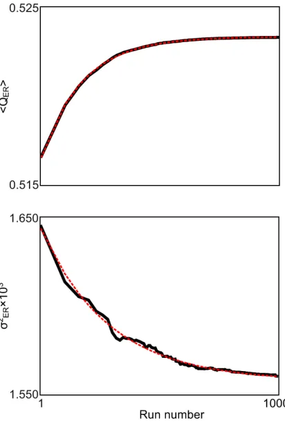
Figure 2.Convergence of modularity distribution for an ensemble of ER graphs withN= 50andp= 0.06. The top panel shows the best modularity measured after a given number of runs; the bottom panel shows the respective variance. The dashed red lines are power-law fits to the measured data.
with the best result amongst known methods. The results are shown in Table 1. For each network we ran our algorithm a number of times, and the best result we obtained is what is reported in the Table. In each case, the best result was obtained within the first one hundred runs. For the time estimates, we ran our algorithm on a single core of an affordable, stand-alone workstation with a single IntelR
CoreTM i5-2400 CPU and 4 GB of RAM. The processor is, at the time of writing, almost 4 years old, having been introduced by the manufacturer in January 2011. In all cases considered, no other fast modularity maximizing algorithm finds a more modular network partition than the one identified by our method. In fact, there are no reported results even from simulated annealing, a slow algorithm, that exceed ours.
4. Estimating the effect size
< QE
R
>
0 0.5 1
p
[image:11.612.174.373.108.262.2]10−2 10−1 100
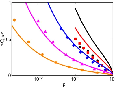
Figure 3. Expected maximum modularity for ER ensembles. The numerical data for N = 10(black dots), 20 (red squares), 50 (blue diamonds), 200 (pink triangles) and 1000 (orange stars) show that the predictions of Eq. 7 (like-coloured lines) are accurate mostly for large dense networks.
quentities, we start from the results in Refs. [26, 27, 28], which provide an estimate of
hQERifor a generic ER ensembleG(N, p):
hQERi= 0.97
r
1−p
N p . (7)
However, the equation above was derived under the assumptions that N ≫ 1 and
p∼1. In other words, the estimate is expected to be valid for large dense networks. Nevertheless, in many real-world systems, networks are typically sparse [47], and often their size is only few tens of nodes [36, 41, 43]. Therefore, to ensure the applicability of Eq. 7, it is necessary to find appropriate scaling corrections. Finding such corrections analytically is a very difficult problem. Thus, here we employ a numerical approach.
First of all, to measure hQERi and σER, we performed extensive numerical simulations, generating ensembles of Erdős-Rényi random graphs withN between 10 and 1000 and p between 1/N and 1. Then, we applied the algorithm described in Section 3 to each network in each ensemble. However, as we discussed before, the algorithm incorporates several elements of randomness. In principle it can give a different result every time it is run. Thus, to estimate the expected maximum modularity for each choice of N and p, we ran the algorithm 1000 times on each network, recording after each runrthe largest value of modularity obtained thus far, and computed ensemble averages ofhQERi(r) andσ2ER(r). The results show a fast convergence of the quantities to their asymptotic value. To model this convergence, we postulate that the difference between the observed value and the asymptotic one decays like a power-law with the number of runsr:
hQERi(r) =hQERi −Ar−B,
σ2ER(r) =σ2ER−Cr−D.
< QE
R
>
0 0.5 1
p
[image:12.612.174.373.108.262.2]10−2 10−1 100
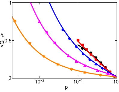
Figure 4. Scaling corrections for expected maximum modularity. The predictions of Eq. 12 are accurate throughout the range of p, and for all system sizes. The numerical data shown are for N = 10 (black dots), 20 (red squares), 50 (blue diamonds), 200 (pink triangles) and 1000 (orange stars).
Figure 3 shows the final numerical results forhQERi, with the predictions of Eq. 7 for comparison. For small system sizes, the measured modularity is lower than that its theoretical prediction. For larger systems, however, the approximation is effectively in agreement with simulations, expect for lower values ofp, in the vicinity of the giant component transition. This suggests the correction we need is twofold, consisting of a multiplicative piece to scale down the prediction for small systems, and an additive piece to account for the case of sparse networks. Thus, an Ansatz for the corrected form is
hQERi=C1·0.97
r
1−p
N p +C2. (8)
The simulation results seem to quickly approach the prediction of Eq. 7 with increasing system size. Therefore, we assume thatC1 is of the form
C1= 1−λe−
N N0 .
Fitting these two parameters with the high-ptail of the results yields
λ = 7
5 ,
N0= 50
Therefore, the multiplicative correction is
C1= 1−7
5e
−N
50 . (9)
The additive piece of the correction clearly depends onpandN. Thus, we start by assuming the general form
C2=C0pα(1−p)βNγ, (10)
where the exponentsα,β, andγ may depend onN. Fitting these parameters yields
σ
2 E
R
10−9
10−8
10−7
10−6
10−5
10−4
10−3
10−2
10−1
p
[image:13.612.177.374.108.252.2]10−2 10−1 100
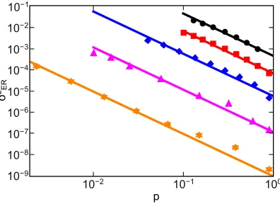
Figure 5. Variance of the expected maximum modularity for ER ensembles. The numerical data for N = 10(black dots), 20 (red squares), 50 (blue diamonds), 200 (pink triangles) and 1000 (orange stars) show that the predictions of Eq. 17 (like-coloured lines) are accurate mostly for small sparse networks.
α =−1
6log
2 5N
β = 5
4
γ =−6
5 + 13 15e
−N
100 .
(11)
To obtain the corrected expression for the expected maximum modularity, substitute the parameter values into Eq. 10, then substitute Eq. 10 and Eq. 9 into Eq. 8:
hQERi=
1−7
5e
−N
50
0.97
r
1−p
N p +p
−1
6log(25N) (1−p) 5 4N−65+
13 15e
−N
100
. (12)
The predictions of Eq. 12, shown in Fig. 4, show a very good agreement for all system sizes and all values ofp. However, to compute thez-score of a given modularity measurement on a particular network, we need to be able to express also the variance of the modularity in the null model of choice. To do so, we first use Eq. 7 to find the expected form of the variance, using propagation of uncertainties. Notice, however, that Eq. 7 was originally derived in the framework of theG(N, m)ensemble, in which the number of nodes N and the number of edges m are held fixed, rather than in theG(N, p)ensemble. Therefore, in finding an equation for the variance ofhQERi,p cannot be considered constant. Then,
σ2hQERi= (∂phQERi)
2
σp2. (13)
Withmfixed, one can writep= 2m N2, hence
σ2p= (∂mp)2σm2 = 4
N4σ
2
m. (14)
Asmis binomially distributed, its variance is
σ2m=
N2
σ
2 E
R
10−9
10−8
10−7
10−6
10−5
10−4
10−3
10−2
10−1
p
[image:14.612.176.374.108.252.2]10−2 10−1 100
Figure 6. Scaling corrections for variance of expected maximum modularity. The predictions of Eq. 18 represent a substantial improvement for anypand all system sizes. The numerical data shown are for N = 10(black dots), 20 (red squares), 50 (blue diamonds), 200 (pink triangles) and 1000 (orange stars).
Substituting Eq. 15 into Eq. 14 yields
σ2p= 2
Np(1−p). (16)
Finally, substituting Eq. 16 into Eq. 13 one obtains
σ2hQERi= 0.972
2 1
N3p2. (17)
Once more, the results of the numerical simulations, shown in Fig. 5, indicate that the actual variance deviates from the theoretical prediction. Thus, also in this case we need to find a correction. The deviation of the measured variances from those predicted by means of Eq. 17 rapidly increases with the size of the network, apparently converging towards a constant. Therefore, we postulate that the correction C′ to
Eq. 17 is multiplicative and has the form
C′ =C0′ −e−ε(N−N0). A fit of these parameters gives C′
0 = 2, ε = 501 and N0 = 10. Thus, the final expression for the variance of the expected maximum modularity in aG(N, p) Erdős-Rényi ensemble is
σ2hQERi=
2−e−(N−10)/500.97 2
2 1
N3p2. (18)
Again, the predictions of Eq. 18, shown in Fig. 6, are in very good agreement with the numerical simulations. We note, however, that for values of p greater than approximately 0.15 the numerically measured variance deviates slightly from the predicted behaviour. In this region, we appear to slightly overestimate the magnitude of the z-score. We postulate, however, that this is due to an increased hardness in finding the best partition for networks having this range of connectivity. Assuming this is case and our prediction of the variance is correct in this region, our estimate of the magnitude of thez-score is accurate throughout the range.
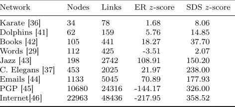
Table 2. Null model motivation. Adopting as the null model the ensemble of networks with the same degree sequence (SDS) as the one studied always results in a more positivez-score, indicating an underestimation of the expected maximum modularity in the SDS ensemble. The networks used here are the same we used for the results shown in Table 1.
Network Nodes Links ERz-score SDSz-score
Karate [36] 34 78 1.68 8.06
Dolphins [41] 62 159 5.76 14.85 Books [42] 105 441 18.27 37.70
Words [29] 112 425 -3.51 2.07
Jazz [43] 198 2742 108.91 150.20 C. Elegans [37] 453 2025 21.97 238.00 Emails [44] 1133 5045 70.89 177.93 PGP [45] 10680 24316 -144.17 326.00 Internet[46] 22963 48436 -217.95 358.52
Eq. 2. Then, one uses Eqs. 12 and 18, to calculate hQERi and σER, respectively. Finally, using these values, Eq. 3 yields thez-score.
To further motivate the choice of the Erdős-Rényi random graph ensemble as the natural null model for network partitioning, we used the degree-based graph sampling algorithm of Ref. [31] to construct ensembles of networks with the same degree sequences (SDS) as the benchmark systems we used for validation. The comparison between the z-scores obtained with the two approaches is shown in Table 2. In all cases, the SDS z-scores are more positive than the ER ones. This strongly suggests that the SDS ensemble underestimates the expected maximum modularity. The reason for this behaviour is in the term−kikj
2m in Eq. 1, which estimates the number of links between a node of degree ki and one of degree kj. This factor implicitly accounts for the possibility of multiple edges in the networks, and therefore its magnitude is larger than it should be. While this overestimate is negligible for ER graphs, it becomes significant for networks with degree distributions different from those of random graphs. The effect is particularly marked on scale-free networks, such as most of the ones we analyzed here, since random networks with a power-law degree distribution are known to be disassortative [48, 49]. These considerations suggest that the ER ensemble is the correct null model to use for the calculation of z-scores for modularity-based algorithms in most community detection applications.
5. Conclusions
measures the effect size of modularity.
The conversion from modularity value to the z-score of modularity effect size we have established is particularly noteworthy. Because of it, for the first time, one can easily estimate the relative importance of the modular structure in networks with different numbers of nodes or links. This allows a new form of comparative network analysis. For example, Table 1 lists the modularity z-scores of the real-world test networks we used to validate our algorithm. Note that most of the networks have a
z-score much greater than 1, and thus their structure is substantially unlikely to be due to a random fluctuation, with the collaboration network of Jazz musicians being by far the least random of those studied. However, the Key Signing network has a largenegative z-score. Thus, it is substantially less modular than a comparable ER network. This indicates that, even though the network has a very prominent modular structure, as evidenced by the large modularity, its links are nonetheless much more evenly distributed than expected if it were random. Similarly, we can say that the word adjacency network in “David Copperfield” has a slightly less modular structure than expected if random, and the Karate Club network has a modular structure that could still be attributed to a random fluctuation, although with a probability of only about 5%. This form of analysis is clearly much more informative than one that considers modularity alone. The difference is particularly striking, for instance, with the Key Signing network, which has a very high value of modularity, but a much less modular structure than a comparable random network. The deeper level of insight the modularityz-score provides makes it ideal for the investigation of real-world networks, and thus it will find broad application in the study of the Physics of Complex Systems.
Acknowledgments
We would like to thank Florian Greil, Suresh Bhavnani and Shyam Visweswaran for fruitful discussions. ST, AN and KEB acknowledge funding from NSF through Grant No. DMR-1206839, and by the AFOSR and DARPA through Grant No. FA9550-12-1-0405. CIDG acknowledges support by EINS, Network of Excellence in Internet Science, via the European Commission’s FP7 under Communications Networks, Content and Technologies, grant No. 288021.
Appendix A. Computational complexity of the fine-tuning step
To estimate the worst-case computational complexity of the fine-tuning step, we start by rewriting Eq. 5 in vector form:
q{c}=
1 4ms
T·B·s .
In the following, to simplify the derivations, sum is implied over repeated Roman (but not Greek) indices. Then, it is
q≡q{c}=
1
4msiBijsj.
Now, consider switching the community assignment of the αth node. This corresponds to changing the sign of the αth component of s: s
the new state vector is
s′ =s+ ∆s=s+
0 .. . 0
−2sα 0 .. . 0 .
Then, the new value of the modularity is
q′≡q{c′}= 1 4ms
′T·B·s′
= 1 4m s
T·B·s+ ∆sT·B·s+sT·B·∆s+ ∆sT·B·∆s
=q+ 1
4m(−2sαBαjsj−2siBiαsα+ 4sαBααsα)
=q− 1
msαBαisi+
1
mBαα,
where we have used the fact thatB is symmetric ands2 α= 1.
Next, define the vectorW as W ≡B·s, so that its components are
Wi =Bijsj.
Then, we have
q′=q− 1
msαWα+
1
mBαα.
Now, consider making a second change in a component of s, say the βth component, with β 6= α. The change is sβ → −sβ. Thus, the new state vector is
s′′=s+ ∆s′=s+
0 .. . 0
−2sα 0
.. .
0
−2sβ 0 .. . 0 .
Then, the new value of modularity is
q′′≡q{c′′}= 1 4ms
′′T·
B·s′′
= 1 4m s
T·B·s+ ∆s′T·B·s+sT·B·∆s′+ ∆s′T·B·∆s′
=q+ 1
+ 4sαBααsα+ 4sβBβαsα+ 4sαBαβsβ+ 4sβBββsβ)
=q− 1
msαBαisi−
1
msβBβisi+
1
mBαα+
1
mBββ+
2
msβBβαsα
=q′− 1
msβBβisi+
1
mBββ+
2
msβBβαsα
=q′− 1
msβWβ+
1
mBββ+
2
msβBβαsα
=q′− 1
msβW
′
β+ 1
mBββ
where
Wβ′ =Wβ−2Bβαsα.
Generalizing to the(n+ 1)th change,
q(n+1)=q(n)− 1
msα(n+1)W
(n) α(n+1)+
1
mBα(n+1)α(n+1),
where
Wα(n)(n+1)=W
(n−1) α(n+1)−2
n
X
p=1
Bα(n+1)α(p)sα(p).
Note that we need to calculate Wα(n)(n+1) for all possible remaining unchanged
α(n+1). Rewrite this as
Wα(n)(n+1)=W
(n−1) α(n+1)−∆W
(n) α(n+1), where
∆Wα(n)(n+1) = 2
n
X
p=1
Bα(n+1)α(p)sα(p).
But then
∆Wα(n)(n+1)= 2Bα(n+1)α(n)sα(n)+ 2
n−1
X
p=1
Bα(n+1)α(p)sα(p)= 2Bα(n+1)α(n)sα(n)+ ∆W
(n−1) α(n+1)
So, the fine-tuning algorithm can be implemented as follows: (prior knowledge of
qandsis assumed)
(i) CalculateWi(0)=Bijsj for alli. (ii) Calculateq(1)=q+ 1
m
Bββ−sβWβ(0)
for allβ, and choose the one that results in the largest value ofq(1)−q. Define that value ofβ to beα(1).
(iii) Define∆Wi(0)= 0for alli. (iv) Setn= 1.
(v) Calculate∆Wi(n)= ∆Wi(n−1)+ 2Biα(n)sα(n) for alli except
α(1), . . . , α(n) .
(vi) CalculateWi(n)=Wi(n−1)−∆Wi(n)for alliexcept
α(1), . . . , α(n) .
(vii) Calculate q(n+1) = q(n)+ 1 m
Bββ−sβWβ(n)
for all β except
α(1), . . . , α(n) , and choose the one that results in the largest value ofq(n+1)−qn. Define that value ofβ to beα(n+1).
To estimate the computational complexity of the fine-tuning algorithm, consider the complexity of each step:
• Using sparse matrix methods, Step (i) is O(m). Thus, in the worst case, its complexity isO(N2).
• Steps (ii) and (iii) are bothO(N).
• Step (iv) isO(1).
• Steps (v) through (viii) areO(N), but are repeatedO(N)times. Thus, the total worst case complexity of one fine-tuning update isO(N2).
Note that when applying the above treatment to the bisection of a particular module of a network, one should not disregard links involving nodes that do not belong to the module considered. Thus, the degrees of the nodes involved in the calculation should not be changed and should account for all the links incident to them [33].
Appendix B. Computational complexity of the final-tuning step
Consider a nonoverlapping partitioning ofNnodes intorcommunities. Then represent the partitioning as anN×rmatrix S where
Sij=
1 if nodeiis in communityj
0 otherwise.
Then, the modularity is
q= 1
2mTr S
T·B·S
= 1 2mS
T
kiBijSjk= 1
2mSikBijSjk,
again we are implying sum over repeated Roman (but not Greek) indices. Please also note our use of notation in what follows. Indices withαandadesignate one of theN
nodes. Indices with β andb designate one of ther communities. Thus,Sβα andSβi are elements of anr×N matrix, whileSαβ andSiβ are elements of anN×rmatrix. Also, by1αβ we indicate an matrix element 1 in position(α, β). Note that 1βα and 1βi are unit valued elements of an r×N matrix, while 1αβ and1iβ are unit valued elements of anN×rmatrix.
Now, consider making a change in the community assignment of one node, sayα, from communityβ toβ′, withβ′6=β. Then, the new state matrix is
S′=S+ ∆S=S+
0 · · · 0 0 0 · · · 0 0 0 · · · 0
..
. . .. ... ... ... . .. ... ... ... . .. ...
0 · · · 0 −1αβ 0 · · · 0 1αβ′ 0 · · · 0 0 · · · 0 0 0 · · · 0 0 0 · · · 0
..
. . .. ... ... ... . .. ... ... ... . .. ...
0 · · · 0 0 0 · · · 0 0 0 · · · 0
.
Equivalently, we can write
S′=S−∆S−+ ∆S+=S−
0 · · · 0 0 0 · · · 0 0 0 · · · 0
..
. . .. ... ... ... . .. ... ... ... ... ...
0 · · · 0 1αβ 0 · · · 0 0 0 · · · 0 0 · · · 0 0 0 · · · 0 0 0 · · · 0
..
. . .. ... ... ... . .. ... ... ... ... ...
0 · · · 0 0 0 · · · 0 0 0 · · · 0
+
0 · · · 0 0 0 · · · 0 0 0 · · · 0
..
. . .. ... ... ... ... ... ... ... . .. ...
0 · · · 0 0 0 · · · 0 1αβ′ 0 · · · 0 0 · · · 0 0 0 · · · 0 0 0 · · · 0
..
. . .. ... ... ... ... ... ... ... . .. ...
0 · · · 0 0 0 · · · 0 0 0 · · · 0
.
Thus, using the same convention as in the previous appendix, the new value of the modularity is
q′= 1
2mTr S
′T·B·S′
= 1 2mTr S
T·B·S−∆ST
−·B·S+ ∆S+T·B·S−ST·B·∆S−
+ST·B·∆S++ ∆S−T·B·∆S−−∆S−T·B·∆S+
−∆S+T·B·∆S−+ ∆S+T·B·∆S+
=q+ 1 2m −
X
ik
1TαβBijSjkδβk+
X
ik
1Tαβ′BijSjkδβ′k
−X
jk
SikTBij1αβδβk+
X
jk
SikTBij1αβ′δβ′k+
X
ij
1TαβBij1αβδββ
−X
ij
1TαβBij1αβ′δββ′−
X
ij
1Tαβ′Bij1αβδββ′+
X
ij
1Tαβ′Bij1αβ′δβ′β′
=q+ 1
2m(−1βαBαjSjβ+ 1β′αBαjSjβ′−SβiBiα1αβ
+Sβ′iBiα1αβ′+ 2Bαα)
=q− 1
mBαiSiβ+
1
mBαiSiβ′+
1
mBαα,
where we have exploited the fact thatB is symmetric.
Next, define theN×rmatrixW asW ≡B·S, So that its components are
Wik=BijSjk.
Then, we have
q′=q− 1
mWαβ+
1
mWαβ′+
1
mBαα.
Now, consider making a second change in a component ofS. Let’s indicate with
α(1) the first node moved, which switched from community β(1) to β′(1). Then, the second change moves nodeα(2) from communityβ(2) toβ′(2). Note thatα(2) 6=α(1) andβ′(2)6=β(2). The new value of the modularity is
q(2)=q− 1
mBα(1)iSiβ(1)+
1
mBα(1)iSiβ′(1)−
1
mBα(2)iSiβ(2)
+ 1
mBα(2)iSiβ′(2)+
1
mBα(1)α(1)+
1
mBα(2)α(2)
+ 1
2mTr(1β(1)α(1)Bα(1)α(2)1α(2)β(2)+ 1β(2)α(2)Bα(2)α(1)1α(1)β(1)
−1β′(1)α(1)Bα(1)α(2)1α(2)β(2)−1β′(2)α(2)Bα(2)α(1)1α(1)β(1)
+ 1β′(1)α(1)Bα(1)α(2)1α(2)β′(2)+ 1β′(2)α(2)Bα(2)α(1)1α(1)β′(1))
=q− 1
mBα(1)iSiβ(1)+
1
mBα(1)iSiβ′(1)−
1
mBα(2)iSiβ(2)
+ 1
mBα(2)iSiβ′(2)+
1
mBα(1)α(1)+
1
mBα(2)α(2)
+ 1
m(Bα(2)α(1)δβ(2)β(1)−Bα(2)α(1)δβ(2)β′(1)
−Bα(2)α(1)δβ′(2)β(1)+Bα(2)α(1)δβ′(2)β′(1))
=q− 1
mBα(1)iSiβ(1)+
1
mBα(1)iSiβ′(1)−
1
mBα(2)iSiβ(2)
+ 1
mBα(2)iSiβ′(2)+
1
mBα(1)α(1)+
1
mBα(2)α(2)
+ 1
mBα(2)α(1)(δβ(2)β(1)−δβ(2)β′(1)−δβ′(2)β(1)+δβ′(2)β′(1))
=q(1)− 1
mBα(2)iSiβ(2)+
1
mBα(2)iSiβ′(2)+
1
mBα(2)α(2)
+ 1
mBα(2)α(1) δβ(2)β(1)−δβ(2)β′(1)−δβ′(2)β(1)+δβ′(2)β′(1)
=q(1)− 1
mWα(2)β(2)+
1
mWα(2)β′(2)+
1
mBα(2)α(2)
+ 1
mBα(2)α(1) δβ(2)β(1)−δβ(2)β′(1)−δβ′(2)β(1)+δβ′(2)β′(1)
=q(1)− 1
mW
(1) α(2)β(2)+
1
mW
(1) α(2)β′(2)+
1
mBα(2)α(2),
where
Wα(1)(2)β(2)=Wα(2)β(2)−Bα(2)α(1) δβ(2)β(1)−δβ(2)β′(1)
.
Generalizing to the(n+ 1)th change,
q(n+1)=q(n)− 1
mW
(n)
α(n+1)β(n+1)+
1
mW
(n)
α(n+1)β′(n+1)+
1
mBα(n+1)α(n+1)
where
Wα(n)(n+1)β(n+1)=W
(n−1)
α(n+1)β(n+1)−
n
X
p=1
Bα(n+1)α(p) δβ(n+1)β(p)−δβ(n+1)β′(p)
.
Rewrite this as
Wα(n)(n+1)β(n+1) =W
(n−1)
α(n+1)β(n+1)−∆W
(n)
α(n+1)β(n+1), where
∆Wα(n)(n+1)β(n+1)=
n
X
p=1
Bα(n+1)α(p) δβ(n+1)β(p)−δβ(n+1)β′(p)
.
But then it is
∆Wα(n)(n+1)β(n+1)=Bα(n+1)α(n) δβ(n+1)β(n)−δβ(n+1)β′(n)
+ n−1
X
p=1
Bα(n+1)α(p) δβ(n+1)β(p)−δβ(n+1)β′(p)
=Bα(n+1)α(n) δβ(n+1)β(n)−δβ(n+1)β′(n)
So, the final-tuning algorithm can be implemented as follows:
(i) CalculateWab(0)=BaiSib for allaandb.
(ii) Calculateq(1)=q+ 1 m
Baa−Wab(0)+Wab(0)′
, wherebis the starting community of node a, for all a and b′, with b′ 6= b, and choose the one that results in the
largest value ofq(1)−q. Define that value of ato beα(1) and that value ofb′ to
beβ′(1).
(iii) Define∆Wab(0)= 0for allaandb. (iv) Setn= 1.
(v) Calculate ∆Wab(n) = ∆Wab(n−1) + Baα(n) δbβ(n)−δbβ′(n) for all a except
α(1), . . . , α(n) , and allb.
(vi) CalculateWab(n)=Wab(n−1)−∆Wab(n)for allaexcept
α(1), . . . , α(n) , and allb.
(vii) Calculate q(n+1) = q(n) + 1 m
Baa−Wab(n)+Wab(n)′
for all a except
{α(1), . . . , α(n)}, and all b′, and choose the pair that results in the largest value
ofq(n+1)−q(n). Define that value ofato be α(n+1), and thatb′ to beβ′(n+1) (viii) If n+ 1< N, setn=n+ 1and go to step (v).
To estimate the computational complexity of the final-tuning algorithm, consider the complexity of each step:
• Step (i) isO(N2).
• Steps (ii) to (iv) areO(N2).
• Steps (v) to (vii) areO(N2), but are repeatedO(N2)times.
Thus, the worst case computational complexity of a final-tuning update isO(N3).
Appendix C. Computational complexity of the agglomeration step
To find complexity of the agglomeration step, first rewrite the definition of modularity as
q= 1
2m r X k=1
k6=x,y
X
i,j∈Ck
Bij+
X
i,j∈Cx
Bij+
X
i,j∈Cy
Bij
,
where andCxand Cy are two communities to be merged, andr is the total number of communities. Now, merge Cx and Cy into a new community Cz. Then, the new value of the modularity is simply
q′= 1
2m r′ X k=1
k6=z
X
i,j∈Ck
Bij+
X
i,j∈Cz
Bij
,
where r′ =r−1. Now, decompose the contribution to the modularity coming from
communityCz into the contributions of its consitutent communitiesCx andCz:
X
i,j∈Cz
Bij=
X
i,j∈Cx
Bij+
X
i,j∈Cy
Bij+ 2
X
i∈Cx
X
j∈Cy
Therefore, the change in modularityδq=q′−qis
δq= 1
m X
i∈Cx
X
j∈Cy
Bij.
Thus, we can define an r×rmatrix W such that its (i, j)element is the change in modularity that would result from the merger of communitiesCi andCj.
Now, consider merging communities Cr and Cs. If neither community is Cz, then the corresponding change in modularity is the same as it would have been in the previous step. This means that after each merger we only need to update the rows and columns ofW corresponding to the merged communities. Without loss of generality, assume it wasx < y. Then, it is
W′
xi =Wxi+Wyi ∀i6={x, y}
Wix′ =Wix+Wiy ∀i6={x, y} .
So, the agglomeration algorithm can be implemented as follows:
(i) Build the matrix W.
(ii) Find the largest element ofW,Wij, with i < j. (iii) Move all the nodes inCj to Ci.
(iv) Decrease the number of communitiesrby 1. (v) Ifr >1, update W and go to step (ii).
To estimate the computational complexity of the agglomeration algorithm, consider the complexity of each step:
• Step (i) isO(N2).
• Steps (ii) to (iv) areO(N2), but are repeatedO(N)times.
Thus, the computational complexity of an agglomeration step isO(N3).
References
[1] Albert R and Barabási A-L 2002Rev. Mod. Phys.74, 47–97 [2] Newman M E J 2003SIAM Review45, 167–256
[3] Boccaletti Set al.2006Phys. Rep.424, 175–308 [4] Boccaletti Set al.2014Phys. Rep.544, 1–122 [5] Pimm S L 1979Theor. Popul. Bio.16, 144–58 [6] Garnett G Pet al.1996Sex. Transm. Dis.23, 248–57
[7] Flake G W, Lawrence S, Giles C L and Coetzee F M 2002Computer 32, 66–70 [8] Girvan M and Newman M E J 2002Proc. Natl. Acad. Sci. USA99, 7821–26 [9] Eriksen K A, Simonsen I, Maslov S and Sneppen K 2003Phys. Rev. Lett.90, 148701 [10] Krause A Eet al.2003Nature426282–85
[11] Lusseau D and Newman M E J 2004P. Roy. Soc. Lond. B. Bio.271, S477–81 [12] Guimerà R and Amaral L A N 2005Nature433, 895–900
[13] Del Genio C I and Gross T 2011New J. Phys.13, 103038
[14] Treviño S, Sun Y, Cooper T and Bassler K E 2012PLoS Comp. Bio.8, e1002391 [15] Palla G, Derényi I, Farkas I and Vicsek T 2005Nature435, 814–8
[16] Huss Met al.2007IET Syst. Biol.1, 280
[17] Restrepo J G, Ott E and Hunt B R 2006Phys. Rev. Lett.97, 94102
[18] Arenas A, Díaz-Guilera A and Pérez-Vicente C J 2006Phys. Rev. Lett.96, 114102 [19] Del Genio C I and House T 2013Phys. Rev. E88, 040801(R)
[20] Díaz-Guilera A, Duch J, Arenas A and Danon L 2007 inLarge scale structure and dynamics of complex networks (Singapore: World Scientific), 93–114
[23] Chen M, Kuzmin K and Szymanski B K 2014IEEE Trans. Computation Social System1, 46–65 [24] Sobolevsky S, Campari R, Belyi A and Ratti C 2013Phys. Rev. E 90, 012811
[25] Brandes Uet al.2008IEEE Trans. Knowl. Data Eng.20, 172–88 [26] Reichardt J and Bornholdt S 2006Phys. Rev. E 74, 016110 [27] Reichardt J and Bornholdt S 2006Physica D224, 20–6 [28] Reichardt J and Bornholdt S 2007Phys. Rev. E 76, 015102 [29] Newman M E J 2006Phys. Rev. E74, 036104
[30] Erdős P and Rényi A 1960A Matematikai Kutató Intézet Közleményei 5, 17–60 [31] Del Genio C I, Kim H, Toroczkai Z and Bassler K E 2010PLoS One5, e10012 [32] Kim H, Del Genio C I, Bassler K E and Toroczkai Z 2012New J. Phys.14, 023012 [33] Newman M E J 2006Proc. Natl. Acad. Sci. USA103, 8577–82
[34] Kernighan B and Lin S 1970Bell Syst. Tech. J 49, 291–307 [35] Sun Y, Danila B, Josić K and Bassler K E 2009EPL86, 28004 [36] Zachary W W 1977J. Anthropol. Res.33, 452–73
[37] Duch J and Arenas A 2005Phys. Rev. E 72, 027104
[38] Noack A and Rotta R 2009Lect. Notes Comput. Sc.5526, 257–68 [39] Good B H, de Montjoye Y-A and Clauset A 2010Phys. Rev. E 81, 046106
[40] Le Martelot E and Hankin C 2011 Proceedings of the 2011 International Conference on Knowledge Discovery and Information Retrieval 216–25
[41] Lusseau Det al.2003Behav. Ecol. Sociobiol.54, 396–405 [42] http://www.orgnet.com/divided.html
[43] Gleiser P M and Danon L 2003Adv. Complex Syst.6, 565–73 [44] Guimerà Ret al.2003Phys. Rev. E 68, 065103(R)
[45] Boguñá M, Pastor-Satorras R, Diaz-Guilera A and Arenas A 2004 Phys. Rev. E 70, 056122 (2004)
[46] http://www-personal.umich.edu/~mejn/netdata/as-22july06.zip