Time varying brain connectivity with multiregression dynamic models

(1)

warwick.ac.uk/lib-publications

A Thesis Submitted for the Degree of PhD at the University of Warwick

Permanent WRAP URL:

http://wrap.warwick.ac.uk/101426

Copyright and reuse:

This thesis is made available online and is protected by original copyright.

Please scroll down to view the document itself.

Please refer to the repository record for this item for information to help you to cite it.

Our policy information is available from the repository home page.

(2)

Time-Varying Brain Connectivity with

Multiregression Dynamic Models

by

Ruth Harbord

Thesis

Submitted to the University of Warwick

for the degree of

Doctor of Philosophy

MOAC Doctoral Training Centre, University of Warwick

September 2017

1 2

(3)

List of Tables

1.1 The LiNG family of algorithms. . . 27

3.1 Estimated run time of the MDM-DGM, per subject, per node, for

in-creasing numbers of nodes. . . 55

3.2 Computational complexity of the Dynamic Linear Model . . . 56

3.3 Stepwise methods dramatically reduce the number of models to score. . . 57

(8)

List of Figures

1.1 Example graphs for a 3 node network. . . 7

1.2 The probability distribution associated with a Bayesian network can be expressed in terms of a set of conditional probabilities. . . 8

1.3 Example of Markov equivalent graphs. . . 8

1.4 Inferring connectivity strengths with path analysis. . . 10

1.6 Illustration of the PC algorithm . . . 24

1.7 Procedures for edge orientation based on measures of non-Gaussianity . . 27

1.8 Illustration of the MDM-IPA . . . 31

2.1 The optimal discount factor δ(r) for each subject across nodes and ex-perimental conditions. . . 35

2.2 The number of parents for each subject across nodes and experimental conditions. . . 35

2.3 Partial correlation and DGM estimate similar networks but MDM-DGM also infers directionality. . . 37

2.4 MDM-DGM networks are similar for the ‘safe’ and ‘anticipation of shock’ conditions . . . 39

2.5 Edges shared by>90 % of subjects for the (a) ‘safe’ and (b) ‘anticipation of shock’ datasets. . . 40

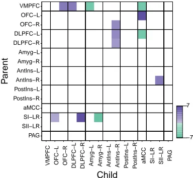
2.6 Evidence for a difference between the ‘safe’ and ‘anticipation of shock’ conditions . . . 41

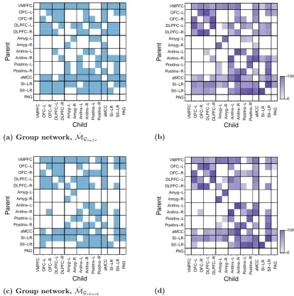
2.7 MDM-DGM group networks for the ‘safe’ and ‘anticipation of shock’ datasets . . . 43

(9)

2.9 Evidence for a difference between the group and individual subject

net-works . . . 46

2.10 The state vector ˆθt(r) provides a measure of connectivity strength. . . . 47

2.11 A paired t-test does not find a significant difference in the connectivity strengths for the ‘safe’ and ‘anticipation of shock’ datasets. . . 49

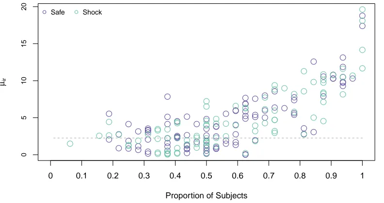
2.12 Edges shared by a high proportion of subjects have stronger connectivity strengths . . . 49

2.13 Differences between the ‘safe’ networks when the subjects are split based on induced and trait anxiety . . . 50

2.14 Differences between the ‘anticipation of shock’ networks when the sub-jects are split based on induced and trait anxiety . . . 51

3.1 Illustration of stepwise algorithms for the MDM-DGM . . . 58

3.2 The performance of forward selection . . . 61

3.3 The performance of backward elimination . . . 62

3.4 Loge Bayes factor comparison between the parent sets discovered by ex-haustive and forward selection and exex-haustive and backward elimination searches . . . 63

3.5 Combining forward selection and backward elimination . . . 64

3.6 Loge Bayes factor comparison between the parent sets discovered by exhaustive and combined forward selection and backward elimination searches. . . 65

3.7 The accuracy of the stepwise approaches decreases as the number of nodes increases. . . 67

3.8 The loge Bayes factor for the highest scoring vs. the next highest scoring model decreases as the number of nodes increases. . . 67

3.9 The number of models with equivalent evidence increases as the number of nodes increases, but decreases as a percentage of the model space . . . 68

4.1 Correspondence between the consistency of edge presence and connec-tivity strength for the aMCC . . . 71

(10)

4.3 Illustration of the influence of a non-local prior on the loge Bayes factor

and posterior model probabilities. . . 74

4.4 Examples of a univariate product moment non-local prior. . . 78

4.5 The time-varying regression coefficient for the edge DLPFC-L→OFC-L

in the model with parents VMPFC, DLFPC-L and Amyg-L. . . 80

4.6 Example of a DLM-QF non-local prior. . . 82

4.7 Correspondence between the consistency of edge presence and

connec-tivity strength for the OFC-L subnetwork . . . 87

4.8 As the number of parents increases, the discount factor δ(r) tends to-wards higher values . . . 90

4.9 Under a DLM-pMOM prior, the optimum δ(r) is higher than under a local prior. . . 90

4.10 The effect of the discount factorδ(r) on the strength of the penalty . . . 91 4.11 Values of the posterior scale parameter C∗_T(r) across subjects for each

parent in the subnetwork . . . 92

4.12 The influence of the prior hyperparameter C∗₀(r) on the estimates for the regression coefficients . . . 93

4.13 The influence of the prior hyperparameterC∗₀(r)on the strength of the penalty . . . 94

(11)

Acknowledgements

First and foremost, I would like to express my gratitude to my supervisor Prof. Tom Nichols for giving me the opportunity to pursue this project and for his ongoing

guid-ance and support.

I would also like to thank the NeuroStat group at the University of Warwick (now the NISOx group at the University of Oxford). I am particularly grateful to Dr. Simon

Schwab for his help with developing the MDM-DGM code. I would also like to thank

Dr. Lilia Costa for providing the original code.

My extended thanks go to Prof. Jim Smith for his advice on the MDM and Prof. David

Rossell, for going above and beyond to help me understand non-local priors. I would

also like to thank Dr. Janine Bijsterbosch and Dr. Sonia Bishop for sharing their data with me.

I would like to thank my examiners, Prof. Will Penny and Dr. Theo Damoulas, for

their detailed and helpful feedback.

Within the MOAC Doctoral Training Centre, my heartfelt thanks go to Prof. Alison Rodger for giving me the chance to undertake a PhD and her continued faith in me.

I gratefully acknowledge financial support from the Engineering and Physical Sciences

Research Council that made my PhD possible. I would also like to thank Dr. Hugo van den Berg, for his ongoing advice and for many interesting conversations over the years.

I would like to thank my MOAC cohort, in particular my office buddies Katherine

(12)

Declaration

This thesis is submitted to the University of Warwick in support of my application for the degree of Doctor of Philosophy. It has been composed by myself and has not been

submitted in any previous application for any degree. Where I have drawn on the work of others, this is clearly attributed.

The work presented (including data generated and data analysis) was carried out by

the author except in the case outlined below:

Preprocessed functional MRI datasets were provided by Dr. Janine Bijsterbosch, The FMRIB Centre, University of Oxford.

Parts of this thesis have appeared in

Harbord, R. et al., (2016), Scaling up Directed Graphical Models for Resting-State

fMRI with Stepwise Regression 22nd Annual Meeting of the Organization for Human

Brain Mapping, Geneva, Switzerland.

Harbord, R. et al., (2015), Dynamic Effective Connectivity Modelling of Pain with

Multiregression Dynamic Models 21st Annual Meeting of the Organization for Human

Brain Mapping, Honolulu, Hawaii.

Code for the MDM-DGM search was originally provided by Dr. Lilia Costa and has

been optimised and extended by the author in collaboration with Dr. Simon Schwab.

Functions for both exhaustive and stepwise MDM-DGM searches are available in the

multdyn package for R1,2.

1

R Core Team.R: A Language and Environment for Statistical Computing. R Foundation for Statistical

Computing, Vienna, Austria, 2017. URLhttps://www.R-project.org/

2

Schwab, S., Harbord, R., Costa, L., and Nichols, T. multdyn: Multiregression Dynamic Models, 2017a.

(13)

Abstract

Functional magnetic resonance imaging (fMRI) is a non-invasive method for studying the human brain that is now widely used to study functional connectivity. Functional

connectivity concerns how brain regions interact and how these interactions change over time, between subjects and in different experimental contexts and can provide

deep insights into the underlying brain function.

Multiregression Dynamic Models (MDMs) are dynamic Bayesian networks that describe

contemporaneous, causal relationships between time series. They may therefore be applied to fMRI data to infer functional brain networks. This work focuses on the MDM

Directed Graph Model (MDM-DGM) search algorithm for network discovery. The Log

Predictive Likelihood (model evidence) factors by subject and by node, allowing a fast, parallelised model search. The estimated networks are directed and may contain the

bidirectional edges and cycles that may be thought of as being representative of the

true, reciprocal nature of brain connectivity.

In Chapter 2, we use two datasets with 15 brain regions to demonstrate that the

MDM-DGM can infer networks that are physiologically-interpretable. The estimated

MDM-DGM networks are similar to networks estimated with the widely-used partial correlation method but advantageously also provide directional information. As the

size of the model space prohibits an exhaustive search over networks with more than

20 nodes, in Chapter 3 we propose and evaluate stepwise model selection algorithms that reduce the number of models scored while optimising the networks. We show that

computation time may be dramatically reduced for only a small trade-off in accuracy. In

Chapter 4, we use non-local priors to derive new, closed-form expressions for the model evidence with a penalty on weaker, potentially spurious, edges. While the application

of non-local priors poses a number of challenges, we argue that it has the potential to

(14)

Abbreviations

aMCC Anterior mid-cingulate cortex

Amyg Amygdala

AntIns Anterior insula

BE Backward elimination

BOLD Blood-Oxygenation-Level Dependant

DAG Directed Acyclic Graph

DCG Directed Cyclic Graph

DCM Dynamic Causal Modelling

DLM Dynamic Linear Model

DLPFC Dorsolateral prefrontal cortex

fMRI Functional Magnetic Resonance Imaging

FS Forward selection

LPL Log Predictive Likelihood

MDM Multiregression Dynamic Model

MDM-DGM Multiregression Dynamic Model Directed Graph Model

MDM-IPA Multiregression Dynamic Model Integer Programming Algorithm

OFC Orbitofrontal cortex

PAG Periaqueductal gray

PostIns Posterior insula

pMOM Product moment

SI Primary somatosensory cortex

SII Secondary somatosensory cortex

SEM Structural Equation Model

SVAR Structural Vector Autoregression

(15)

Chapter 1

Inferring Brain Connectivity with Functional MRI

1.1 Introduction

Functional Magnetic Resonance Imaging (fMRI) is a neuroimaging modality that offers

a number of advantages: it is non-invasive and allows whole-brain coverage. It has high spatial resolution and relatively high temporal resolution, meaning the brain may be

imaged in almost real time. Subsequently, fMRI has become a widely-used technique for examining both normal and pathological human brain function.

A century of neuroscience research has established that at the macroscopic level the

brain is organised into a collection of distinct anatomical regions, each with its own

highly specialised function. This specialisation has been referred to as functional

seg-regation (Friston et al., 2013). One example is the visual cortex, where it has long

been established that different aspects of an image (e.g. colour, motion, orientation)

are processed separately in different cortical areas (Zeki and Shipp, 1988). Communica-tion within and between these localised, specialised regions has been termedfunctional

integration and is achieved through the extensive afferent, efferent and intrinsic

myeli-nated axonal nerve fibres that compose the structural architecture of the brain (Zilles and Amunts, 2015). Deeper insights may be obtained by considering the activation and

communication of brain regions over time, during a particular task or at rest. Func-tional MRI, in combination with appropriate statistical models, provides a powerful

tool for inferring time-varying patterns of brain connectivity.

1.2 Thesis Outline

A typical fMRI scan measures the activity of a set of anatomical regions over the

course of a few minutes (see the next section for more details). A number of method-ologies have been developed which aim to infer brain connectivity from this type of

data. Network models treat the brain as a collection of nodes (anatomical regions) and

edges (connections between regions) and provide a powerful framework to model both structural and functional connectivity (Sporns, 2014). Approaches based on network

modelling range from simple descriptions of the data to detailed models with a definite

biophysical interpretation (Smith, 2012).

(16)

deeper insights may be obtained with models that also estimate the orientation of

connections (i.e. the direction of information flow). Methods which allow bidirectional

edges and cycles (thereby modelling feedback loops) may be desirable as they are likely to be more representative of the underlying brain function. Some models of brain

connectivity also provide an estimate of the strength of the influence of one region over

another. If these estimates are dynamic, it is possible to model how the strength of the influence changes over time. It may also be advantageous to be able to estimate

networks and (potentially dynamic) connectivity strengths for individual subjects, as

well as at the group level.

Costa (2014) developed two algorithms for network discovery using fMRI, based on

the Multiregression Dynamic Model (MDM) of Queen and Smith (1993). The

MDM-Integer Programming Algorithm IPA) and MDM-Directed Graph Model (MDM-DGM) searches may be used to infer networks and provide dynamic connectivity

esti-mates both for individual subjects and at the group level. These connectivity estiesti-mates

are the regression coefficients of a Dynamic Linear Model (West and Harrison, 1997). While the MDM-IPA constrains each network to be a directed acyclic graph (DAG),

the MDM-DGM permits cycles and bidirectional edges. Using simulated data, Costa

et al. (2015) showed the MDM-IPA could perform as well as, or better than, a number of competing methods for inferring the presence and direction of edges. The MDM-IPA

and MDM-DGM algorithms were also applied to real fMRI data with 11 brain regions

(Costa, 2014; Costa et al., 2015, 2017).

Focusing on the MDM-DGM, in this thesis we extend the work of Costa (2014) and

Costa et al. (2015, 2017) in a number of directions. To further explore the behaviour of

the MDM-DGM search on real data, we made use of two fMRI resting-state datasets. The original experiment was designed to explore differences in connectivity between

brain regions, specifically relating to trait and induced anxiety. Previous analysis of

this data was reported in Bijsterbosch et al. (2015). We began by validating the MDM-DGM search by comparing the estimated networks with partial correlation networks as

partial correlation is an established method for edge detection (see section 1.5.1). Given

the close correspondence of the networks estimated by these two methods, we used two advantageous features of the MDM-DGM, the ability to infer the orientation of edges

and the ability to provide time-varying connectivity weights, in order to further explore

the role of certain brain regions in trait and induced anxiety. Results are presented in Chapter 2.

To gain fundamental insights into brain function, it is desirable to work with networks

with much larger numbers of brain regions than have typically been used in models of directed connectivity. However, as will be discussed in Chapter 3, the most significant

limitation in terms of the computational complexity of the MDM-DGM algorithm is the

size of the model space, which increases exponentially with the number of brain regions. Using stepwise regression methods, forward selection and backward elimination, the

(17)

methods therefore have the potential to allow the extension of the MDM-DGM to much

larger networks. The performance of these algorithms is assessed in Chapter 3.

MDM-DGM fMRI networks (which we will present in Chapter 2) tend to contain a

number of connections which occur inconsistently across subjects and have low connec-tivity strengths. We hypothesised that these connections were potentially spurious. In

order the increase the sparsity of the networks, we considered non-local priors (Johnson and Rossell, 2012; Rossell and Telesca, 2017) to include a penalty on the model

evi-dence for unnecessarily complex models. One advantageous feature of non-local priors

is that the expressions for the penalised model evidence are closed-form. However, this approach also presents a number of theoretical and computational challenges, as will

be discussed in Chapter 4.

This chapter introduces the use of functional Magnetic Resonance Imaging to infer

dynamic, directed brain activity. For the remainder of this section, some of the key concepts are introduced, including the basic physiology behind the fMRI signal, the

nature of functional brain networks and the insights into brain function that may be possible with this type of inference. In section 1.3, some of the methods that have been

developed to date are outlined, with a particular focus on Bayesian networks and

state-space models. The Multiregression Dynamic Model and the Dynamic Linear Model, which will be the focus of this work, are described in detail in section 1.4. Section 1.5

reviews some commonly-used algorithms for network discovery with fMRI data and our

search procedure, the MDM Directed Graph Model (MDM-DGM) search, is outlined in section 1.6. Further discussion of the MDM-DGM, with a particular focus on the

inference of graphs with cycles, is provided in section 1.7.

1.2.1 BOLD fMRI and Resting-State Networks

Functional MRI measures the blood oxygenation level-dependent (BOLD) contrast.

Increased neuronal activity causes increased cerebral blood flow (CBF), increased cere-bral blood volume (CBV) and oxygen consumption (CMRO2). The increase in cerebral

blood flow is greater than the increased oxygen consumption, resulting in a decrease

in the total amount of deoxygenated hemoglobin (dHb). As deoxyhemoglobin is para-magnetic, the magnetic resonance signal is reduced in its vicinity, so a decrease in

dHb results in a positive BOLD contrast. For a detailed review of the origins of the BOLD signal, see Mark et al. (2015). The BOLD signal is a hemodynamic response

to neuronal activity, occurring at much slower timescales (hundreds of milliseconds to

seconds) than the activity of the underlying neurons which occurs at the millisecond scale (Shmuel and Maier, 2015). This hemodynamic response is known to vary between

cortical regions, subjects and experimental paradigms (Handwerker et al., 2012) and

the exact mechanisms behind the coupling of neural activity, metabolism and hemody-namics are still an active area of research (for reviews see Ugurbil (2016) and Keilholz

et al. (2017)).

(18)

energy is used on spontaneous activity, rather than task-based responses (Fox and

Raichle, 2007). This has motivated the field of resting-state fMRI, where patterns

of activity that are biophysically-meaningful and reproducible across subjects may be extracted from the scans of people at rest rather than engaged in a particular task.

Spontaneous infra-slow (<0.1 Hz) fluctuations in the BOLD response were shown to be strongly correlated between the motor cortices by Biswal et al. (1995) and since then a number of resting-state networks have been identified. In these networks, brain regions

can interact strongly even though they may be spatially-distant. Resting-state networks

not only show a strong correspondence with task-activation networks (Smith et al., 2009), but have been used to successfully predict task-based activation for individual

subjects (Tavor et al., 2016).

There is strong evidence that resting-state fMRI has a neural basis. Keilholz (2014) provides a review of the use of electrophysiological techniques such as EEG

(electroen-cephalography) and invasive intracranial recordings to explore the relationship between

patterns of resting-state BOLD connectivity and the underlying neuronal processes. The relationship between BOLD response and the underlying electrophysiology is

com-plex and it is likely that the BOLD signal arises from multiple electrophysiological

processes. Resting-state networks have been found to have distinct spectral ‘finger-prints’, composed of multiple frequency bands of the EEG signal (Mantini et al., 2007)

and resting-state connectivity patterns (correlation matrices) from (intracranial)

elec-trocorticography recordings have been shown to correlate with fMRI data (Foster et al., 2015).

Using resting-state fMRI and diffusion spectrum imaging, a non-invasive method for

determining structural (anatomical) connectivity, as well as a computational model, Honey et al. (2009) showed that structural connectivity was a good predictor of

resting-state connectivity. Cortical regions that were connected anatomically exhibited stronger

and more consistent resting-state connectivity when compared with anatomically un-connected regions. However, the reverse was not true, resting-state connectivity was

an unreliable predictor of the underlying structural connectivity.

1.2.2 Functional vs. Effective Connectivity

The discovery of synchronised temporal activity across spatially-distant brain areas has given rise to the field of resting-state fMRI connectivity with a large body of research

dedicated to the development and validation of methods for resting-state connectivity

analysis. These methods range from simple descriptions of the data (e.g. full and partial correlation methods) to detailed biophysical models, which map the underlying neural

activity to the observed hemodynamic response (Smith, 2012). Some of these

meth-ods will be reviewed later in this chapter. Central to fMRI connectivity modelling is the distinction betweenfunctional andeffective connectivity, first described by Friston

et al. (1993). Functional connectivity considers statistical dependencies between two

(19)

system over another (Friston et al., 2013). Functional connectivity models

correla-tions between brain regions, so the estimated connectivity isundirected, while effective

connectivity methods are able to make inferences about directed connectivity (Smith, 2012). While methods that include directional information clearly have the potential to

provide a much richer understanding of the data (and the underlying brain function),

these models require careful interpretation, may be computationally-intensive and rely on specific and often different definitions of causality (see, for example, Henry and

Gates (2017) for review).

1.2.3 Dynamic Functional Connectivity

The original research into resting-state functional connectivity assumed that connec-tivity was static over the duration of a typical fMRI scan, i.e. over periods over several

minutes. However, in recent years, evidence has emerged which suggests temporal

dy-namics on much shorter timescales (Chang and Glover, 2010). This has motivated the development of a number of methods which aim to quantify this dynamic functional

connectivity. As the exact relationship between the underlying neural activity and

the observed dynamics in the BOLD signal is still unclear, interpretation of dynamic functional connectivity requires caution. Careful data preprocessing is necessary to

remove the effects of head motion without destroying any true dynamics present in the

BOLD signal (Laumann et al., 2016). Inappropriate statistical analysis can also lead to the erroneous detection of dynamic functional connectivity. Sliding window

meth-ods divide the time series into (sometimes overlapping) intervals and infer dynamics

by comparing the estimated functional connectivity between these intervals. Laumann et al. (2016) used a sliding-window approach to test for dynamic connectivity on BOLD

time series that had been simulated to be stationary, finding that most ‘dynamic’

con-nectivity could be attributed to sampling variability. For a detailed review of dynamic functional connectivity analysis, including discussion of the sliding window method, see

Hutchison et al. (2013). It should also be emphasised that detection of dynamics using

a statistical method does not in itself provide any information about the dynamics of the underlying system (Hindriks et al., 2016).

1.3 Modelling Functional and Effective Connectivity

In this section, we review models for estimating directed connectivity from fMRI data.

This section focuses on model equations and interpretation. The application of some of these models as a basis for network discovery algorithms is reserved until section 1.5.

1.3.1 Bayesian Networks

Inferred directed brain networks from fMRI data relies on a number of concepts from

the field of graphical models. Many of the methods developed to date (including the Multiregression Dynamic Model) are Bayesian network methods. Basic concepts and

(20)

Graphical Models

A graph may be defined by G = {V,E}, where V is some set of vertices ornodes and E is the set of edges (or connections) between the nodes. Two nodes are adjacent if an edge exists between them, e.g. in Figure 1.1a, node 1 and node 2 are adjacent, as

are node 2 and node 3, but node 1 and node 3 are not (i.e. there is no edge between node 1 and node 3). If each node represents a variable, then a graph may be used to

represent interactions between a set of variables. These interactions may be undirected (as in Figure 1.1a) or directed (Figure 1.1b-1.1e), with arrows to denote the direction

of influence. Directed edges can be used to represent causal relationships, so if there is

an arrow from node 1 to node 2, representing the influence of the variable Y(1) on the variable Y(2), we have the interpretation thatY(1)causesY(2). For any directed edge, the node from which the edge originates is called the parent and the node to which the

arrow points is thechild (Spirtes et al., 2000). IfP a(i)and Ch(i) denote the parents and children of node irespectively, then, for example, Figure 1.1c has P a(2) = {1,3},

Ch(1) = {2}and Ch(3) = {2}. If a node has no parents, e.g. node 1 (and node 3), its parent set may be denoted by the empty set asP a(1) = {∅}.

A directed acyclic graph (DAG) is a directed graph which contains no cycles. The

graphs in Figure 1.1b and 1.1c obey the DAG principle. Examples of non-DAGs, or

directed cyclic graphs (DCGs), are shown in Figures 1.1d and 1.1e.

If there is a direct or indirect path from nodeito nodej, nodejis adescendant of node

i(Spirtes et al., 2000). The graph in Figure 1.1b is an example of achain graph, where node 1 influences node 2 which influences node 3. There is anindirect influence of node

1 on node 3 and node 3 is a descendant of node 1. If the influence of node 2 on node 3 is known, the activity of node 3 may be explained without knowledge of node 1. This

may be expressed more formally in terms of conditional independence. Let the graph

in Figure 1.1b be represented by the set of variables Y = {Y(1), Y(2), Y(3)}. The indirect nature of the influence of node 1 is described by the conditional independence

relation

Y(3)

á

Y(1) ∣Y(2)

which may be read as: node 3 is conditionally independent of node 1 given node 2.

Given a set of conditional independence relations, a graph G may be represented by a probability distributionP. A graph and its associated distribution satisfies the Causal

Markov Condition if and only if for every vertexiinV,iis independent ofV ∖{P a(i)∪

(21)

1 2

3

(a)

Undirected graph

1 2

3

(b)

Directed Acyclic Graphs

1 2

3

(c)

1 2 3

1 2

3

(d)

Directed Cyclic Graphs

1 2

3

(e)

1 2

[image:21.595.87.411.72.350.2]

3

Figure 1.1: Example graphs for a 3 node network.

The Markov condition means the probability distributionP factorises as

p[Y(1), . . . , Y(n)] =

n ∏ i=1

p[Y(i) ∣P a(i)]

where nis the number of nodes in the graphG. If the graph is acyclic, then, for some ordering of the nodes, its probability distribution will obey the Bayesian decomposition

rule, such that it may be expressed as

p[Y(1), . . . , Y(n)] =p[Y(1)]p[Y(2) ∣Y(1)], . . . , p[Y(n) ∣Y(1), . . . , Y(n−1)].

A graph with an associated probability distribution of this form comprise a Bayesian

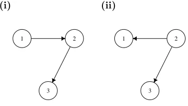
network, B = {G,P}. These concepts are illustrated in Figure 1.2 where a conditional probability may be obtained for each node in the graph as follows

Graph (i) p_Y₍₁₎=p[Y(1) ∣ ∅]

Graph (ii) pY(2) ∣Y(1)=p[Y(2) ∣P a(2)]

Graph (iii) pY(3) ∣Y(1),Y(2)=p[Y(3) ∣P a(3)].

The probability distribution associated with the DAG in graph (iv) is therefore

(22)

(i)

1 2

3

(ii)

1 2

3

(iii)

1 2

3

(iv)

1 2

[image:22.595.93.282.456.563.2]

3

Figure 1.2: The probability distribution associated with a Bayesian network can be expressed in terms of a set of conditional probabilities.

Markov Equivalence

Consider the two graphs in Figure 1.3. Their associated joint probability distributions

are

Graph (i) p[Y(1), Y(2), Y(3)] =p[Y(1)]p[Y(2) ∣Y(1)]p[Y(3) ∣Y(2)]

Graph (ii) p[Y(1), Y(2), Y(3)] =p[Y(1) ∣Y(2)]p[Y(2)]p[Y(3) ∣Y(2)].

Both graphs imply that conditional on node 2, node 1 is independent of node 3. Graphs with the same conditional independence structure are said to be Markov equivalent.

Bayesian networks that are Markov equivalent will have the same skeleton (undirected

graph) (Mumford and Ramsey, 2014). A Bayesian network cannot distinguish between Markov equivalent graphs.

(i)

1 2

3

(ii)

1 2

3

Figure 1.3: Example of Markov equivalent graphs. Graphs are said to be Markov equivalent if they share the same conditional independence relations.

Dynamic Bayesian Networks

An extension is a dynamic Bayesian network. Imagine there areT observations fromn

(23)

a first-order Markovian transition model, the joint probability distribution factors as

p[Y1, . . . ,YT] =p[Y1]

T ∏ t=2

p[Yt∣Yt−1]

=p[Y1]

T ∏ t=2

n ∏ i=1

p[Yt(i) ∣P a(i)t]

whereP a(i)tcontains the parents for nodeiin time-slicetort−1 (Bielza and Larra˜naga, 2014). For a more in-depth discussion, see Costa (2014) and Bielza and Larra˜naga

(2014).

A detailed review of Bayesian networks for fMRI data is provided by Mumford and Ramsey (2014). Some network discovery algorithms which rely on Bayesian network

principles will be reviewed in section 1.5.

1.3.2 Structural Equation Models

Consider the graph in Figure 1.4a. Let this graph represent a system about which some

inference is to be made, i.e. let each node represent a brain region with some activity and each edge an interaction between the regions. The strength of the influence of one

node on another is represented by the connection weightsαandβ. The graph in Figure 1.4a has a corresponding structural equation model (SEM), described by the equations in Figure 1.4b.

The variables of any SEM are split intosubstantive variables and error variables. The

variables represented by each node are the substantive variables and the error terms represent the effect of any causes other than the substantive ones, such as the effect of

exogenous variables. The equations in Figure 1.4b describe a linear SEM. In a linear

SEM, every substantive variable is a linear function of the other substantive variables and its associated error (Spirtes et al., 2000). For example, the edge Y(1) → Y(2) (in Figure 1.4a) means that the variable Y(1) appears in the right hand side of the equation for Y(2):

Y(2) =αY(1) +_Y₍₂₎

so that Y(1) may be described as a direct, substantive cause ofY(2).

More generally, consider a set of nbrain regions, represented by a graph with nnodes. For each region, there is a BOLD time series with length T such that at time t, there is ann×1 vector of observations Y_t⊺= {Y(1), . . . , Y(n)}. This system may be written in matrix form as

Yt=G0Yt+t (1.3.1)

where the n×n matrix G0 is called the path coefficient matrix and is a n×1 error

(24)

1 2

3 α

β

(a) DAG with weighted edges

⎛ ⎜ ⎝

Y(1)

Y(2)

Y(3) ⎞ ⎟ ⎠= ⎛ ⎜ ⎝

0 0 0

α 0 0

0 β 0

⎞ ⎟ ⎠ ⎛ ⎜ ⎝

Y(1)

Y(2)

Y(3) ⎞ ⎟ ⎠+ ⎛ ⎜ ⎝

Y(1)

_Y₍₂₎ Y(3)

⎞ ⎟ ⎠

(b) SEM equations

Figure 1.4: Inferring connectivity strengths with path analysis. A linear structural equation model consists of a graph with a corresponding set of equations. The path coefficient matrix is lower triangular and each entry represents a connectivity strength.

and the absence of a connection is represented by a zero (Penny et al., 2004; Chen et al., 2011). If the path coefficient matrix is lower triangular (as in Figure 1.4b),

the structural equation model will represent a directed acyclic graph. An SEM that

represents a directed acyclic graph is said to be recursive, while a non-recursive SEM may be used to model a directed cyclic graph (Spirtes, 1995).

In an SEM, the presence of an arrow from Y(1) to Y(2) means that Y(1) causes

Y(2). These causal relationships are assumed a priori rather than inferred from the data so SEM methods involve estimating the set of connection strengths represented

by the entries in the matrix G0 (Penny et al., 2004). It is possible to solve for G0 by

rearranging equation 1.3.1 as

Yt=A0t

where the matrixA0= (I−G0)−1 is called themixing matrix. Under certain

assump-tions, this matrix may be estimated by independent component analysis (ICA) and, with appropriate permutation and normalisation, the matrix of connectivity strengths

G0 may be obtained (Shimizu et al., 2006; Lacerda et al., 2012). Algorithms for both

acyclic and cyclic graphs exist and will be discussed in more detail in section 1.5.

1.3.3 Structural Vector Autoregressive Models

Consider two time series from two brain regions Y(1) and Y(2). Let Yt−1(r) be a vector containing all observations from region r up until time t−1, so that we may write Yt−1(1)⊺ = {Y1(1), . . . , Yt−1(1)} and Yt−1(2)⊺= {Y1(2), . . . , Yt−1(2)}. If a better

prediction for Yt(2) at timetcan be obtained usingYt−1(1) than using onlyYt−1(2), then it may be said that Y(1) Granger-causes Y(2) (Granger, 1969; Mannino and

Bressler, 2015). Granger causality is often implemented through vector autoregressive

(VAR) models of the form

Yt=

K ∑ k=1

(25)

where each coefficient matrix Gk describes effects k steps back in time and, as usual,

t is an error vector.

An extension, which combines SEM and VAR models, is the structural vector

autore-gressive (SVAR) model, described by

Yt=G0Yt+

K ∑ k=1

GkYt−k+t

(Hyv¨arinen et al., 2010). Structural equation models describe instantaneous connec-tivity. Let the(j, i)th coefficient of the matrixG0 be denoted byG(₀j,i). The definition

of causality in an instantaneous SEM may be stated as follows: Y(i) causes Y(j) if

G(₀j,i)> 0. Similarly, denote the (j, i)th coefficient of the matrix Gk by G(_kj,i), where this coefficient represents the effect of the variableYt−k(i)on the variableYt(j). Using this framework, Hyv¨arinen et al. (2010) provide a definition of causality for the SVAR

model such that Y(i) is said to cause Y(j) if at least one of the coefficients G(_kj,i)

is significantly non-zero for k≥ 0. Note that Granger causality does not assume any particular underlying causal mechanism (Mannino and Bressler, 2015).

Instantaneous or within-sample connectivity may be thought of as connectivity that occurs at much faster timescales than the temporal resolution of the data (Smith et al.,

2013). Functional MRI causal searches often focus on contemporaneous connectivity. It

was noted by Granger (1969) that causal effects may appear contemporaneous when the data are sampled at much slower rates than the underlying generational process. This

is the case with fMRI data as the underlying neuronal processes occurs at much faster

timescales than the measured BOLD signal, due to the relatively slow hemodynamic response (Henry and Gates, 2017).

1.3.4 State-Space Models

As the BOLD signal is an indirect measure of neuronal activity, models of directed

con-nectivity which only consider the observed response may be unreliable, as the estimated ‘causal’ effects may arise due to variations in the timing of the hemodynamic response,

rather than reflecting a true causal relationship between the brain regions of interest.

As mentioned in section 1.2.1, the hemodynamic response is known to vary between cortical regions, as well as between subjects and populations (Handwerker et al., 2012).

To overcome this, the state-space model framework, which is the focus of this section,

defines directed connectivity in terms of a set of latent or state variables, which may then be related to the measured response. Assume each individual cortical region gives

rise to an individual observation at time t so that for a system with n brain regions,

θ⊺_t = {θt(1), . . . , θt(n)} is an n×1 vector representing some ‘true’ state of the system at time t. Let the state variables θ⊺_t represent the activity of neurons in a cortical area, so that they may be said to represent somequasi-neural variable. The behaviour

(26)

equa-tion. Let there be an n-dimensional random vector Y_t⊺= {Yt(1), Yt(2), . . . , Yt(n)} with a corresponding set of observed valuesy_t⊺= {yt(1), yt(2), . . . , yt(n)}.

Let N (

⋅

,

⋅

) denote the multivariate normal distribution with some mean vector and covariance matrix. A linear dynamical system (LDS) may be described by

Observation equation Yt=Fθt+vt vt∼ N (0,V) (1.3.2a)

State equation θt=Gθt−1+wt wt∼ N (0,W) (1.3.2b)

where G is a n×n state transition matrix, which describes directed interactions be-tween hidden states. The coefficients of the matrixGmay be interpreted as

connectiv-ity strengths, where the diagonal and off-diagonal elements control ‘intrinsic’ (within region) and ‘extrinsic’ (between region) effective connectivity respectively (Kahan and

Foltynie, 2013). The n×nobservation matrix Fdefines a linear relationship between the hidden states and the measured response. Then-dimensional vectorwtis the state evolution noise and the n-dimensional vector vt is the observation noise. Both are assumed to be zero-mean (multivariate) Gaussian with (time-invariant) covariancesW

and V respectively (Roweis and Ghahramani, 1999).

It is possible to define some set of n known, exogenous inputs to the system at time

t, via an n-dimensional vector ut = {ut(1), . . . , ut(n)}. These external inputs might be, for example, the timings of a stimulus presented to a participant in a task-based fMRI study; these external variables are known because they are controlled by the

experimenter. Let the strength of influence of these inputs be determined by an n×n

coefficient matrix D. The state equation 1.3.2b may now be extended to become

θt=Gθt−1+Dut+wt wt∼ N (0,W).

If the coefficient matricesG,DandWare allowed to vary with time, but it is assumed

only a small (<<T) number of distinct matrices exist, indicated by some index swith some associated transition probability p(st = i∣st−1 =j), the state equation becomes

that of the Switching Linear Dynamic System (SLDS) model, developed for BOLD data by Smith et al. (2010) and Smith et al. (2012):

θt=Gstθt−1+Dstut+wt wt∼ N (0,Wst).

The altered neuronal activityθtmay then change the neuronal activity of other regions, via the off-diagonal elements ofG(orGtif this matrix varies with time). These inputs

directly influence the neuronal activity, and may be referred to as driving inputs.

Ad-ditionally, it is also possible to specifymodulatory inputs, which change the underlying neurodynamics (that is, the intrinsic and extrinsic connection strengths) (Penny et al.,

(27)

two different types of input become clear if the state equation is extended as

θt=⎛ ⎝G+

J ∑ j=1

xt(j)Cj⎞

⎠θt−1+Dut+wt wt∼ N (0,W)

This is the state equation of the Multivariate Dynamical Systems (MDS) model of Ryali et al. (2011).

Both of these models operate in a discrete time framework. The LDS state equation

may be expressed in continuous time, see Smith et al. (2013) for a detailed explanation of the parallels between the discrete and continuous time frameworks. Let ˙θ be the

first derivative ofθ andΘbe some set of time-invariant connectivity parameters (Razi

and Friston, 2016). Define Θ= {G˜,C˜1, . . . ,C˜J,D˜,Θh}, where Θh represents the pa-rameters of the hemodynamic model and, following Smith et al. (2013), the ∼notation

indicates continuous time variants of the matrices outlined above. The state equation

of the widely-used, deterministic Dynamic Causal Model (DCM; Friston et al. (2003)) is

˙

θ=⎛

⎝G˜ + J ∑ j=1

u(j)C˜j⎞

⎠θ+Du˜ .

Changes to the rate of change ˙θ are known as second-order or bilinear effects (Kahan and Foltynie, 2013).

θ(1)

θ(2)

G(2,1)

(a) Driving inputs

θ(1)

θ(2)

G(2,1)

G(1,1)

G(2,2)

(b) Modulatory inputs

Figure 1.5: Illustration of a state-space framework for models of effective connec-tivity. The neuronal activity of a regioni is represented by an (unobservable) state variable

θ(i)that varies in discrete or continuous time. (a)Driving inputs directly influence neuronal activity while modulatory inputs(b)affect neuronal activity indirectly by altering the connec-tivity strengths between nodes (the elements of G). See Ryali et al. (2011) and Kahan and Foltynie (2013) for more specific illustrations of MDS and DCM respectively.

(28)

a change in some other region(s), e.g. θt(j) via the coefficient G(j,i). Estimation of causal interactions is then equivalent to the estimation of the coefficient matrices (G,

Gst _{or ˜}_G_{, and} _C

j or ˜Cj, j = 1, . . . , J). These types of models define causality in terms of the effect that one neural system exerts on another, in response to an input.

To extend DCM to resting-state data, where there are no known external inputs, it

becomes necessary to estimate not just the effective connectivity but also the hidden neuronal states that drive the endogenous activity of the system. This may be achieved

with a stochastic DCM where the state equation becomes

˙

θ=⎛

⎝G˜ + J ∑ j=1

ujC˜j⎞

⎠θ+D˜(u+w(

u)_{) +}_w(θ)

and w(θ) and w(u) describe fluctuations in the states and hidden causes respectively

(Li et al., 2011). However, inversion of stochastic models in the time domain is

computationally-intensive. Alternatively, spectral DCM (spDCM) works in terms of the cross-spectra of the observed time series. Rather than estimating the (time-varying)

hidden states, spDCM estimates their (time-invariant) covariance (Friston et al., 2014;

Razi and Friston, 2016).

In order to more fully account for the hemodynamic response, these models replace the

simple linear mapping in equation 1.3.2a by a more biophysically-informed relationship.

For an individual regioni, write

zt(i) = [θt(i), θt−1(i), . . . , θt−L+1(i)]⊺ (1.3.3a)

Yt(i) =b⊺(i)Φ zt(i) +vt(i) vt(i) ∼ N (0, V) (1.3.3b)

where the hemodynamic response is represented by the product b⊺(i)Φ, where b(i)

provides region specific weights for the set of bases contained inΦ. These basis vectors

span most of the variability in observed hemodynamic responses (Penny et al., 2005; Smith et al., 2010). The BOLD response is therefore modelled by the convolution of

the hemodynamic response with the quasi-neural variable θt(i) L steps back into the past plus some zero-mean, uncorrelated, Gaussian observation error (Penny et al., 2005; Ryali et al., 2011). Observation models of this form are used in the SLDS and MDS

models. DCMs, in comparison, use a more complex biophysical model (see Stephan

et al. (2007) for a detailed description).

1.4 Multiregression Dynamic Models

1.4.1 The Multiregression Dynamic Model Equations

Imagine extending the linear dynamical state equations 1.3.2a and 1.3.2b so that the state transition matrix G and the observation matrix F, as well as the state and

observation covariances W and V, may vary with time. As before, for a graph with n

(29)

Yt(r) has a distribution determined by a pr×1 state vector θt(r), so for each node r, there is a linear dynamical system described by

Obs. equation Yt(r) =Ft(r)⊺θt(r) +vt(r) vt(r) ∼ N [0, Vt(r)] (1.4.1a)

state equation θt(r) =Gt(r)θt−1(r) +wt(r) wt(r) ∼ N [0,Wt(r)] (1.4.1b)

where the observation matrixFhas been replaced by a column vector with the same

di-mension asθt(r). Denote the set of observations up to and including timetfor regionr byYt(r)⊺= {Y1(r), . . . , Yt(r)}, where the superscript indicates that we are considering

all observations up to and including time t, rather than an individual time point. Similarly define Xt(r)⊺ = {X1(r)⊺, . . . ,Xt(r)⊺} and Zt(r)⊺ = {Z1(r)⊺, . . . ,Zt(r)⊺} with corresponding vectors of observations xt(r)⊺= {x1(r)⊺, . . . ,xt(r)⊺} and zt(r)⊺ = {z1(r)⊺, . . . ,zt(r)⊺}such that

Xt(r)⊺= {Yt(1), Yt(2), . . . , Yt(r−1)} 2≤r≤n Zt(r)⊺= {Yt(r+1), . . . , Yt(n)} 2≤r≤ (n−1).

The column vector Ft(r) may then be defined as a known but arbitrary function of xt(r)and yt−1(r). It should not depend onzt(r) oryt(r).

Denote a block diagonal matrix byblockdiag{}. DefineGt=blockdiag{Gt(1), . . . ,Gt(n)} and Wt =blockdiag{Wt(1), . . . ,Wt(n)} where Gt(r) is the state matrix for node r and Wt(r) is the state variance for node r. These matrices may depend on past observations xt−1(r) and yt−1(r) but nothing else. The observation variance is de-notedVt(r)such thatVt= {Vt(1), . . . , Vt(n)}. The observation and state error vectors, vt = {vt(1), . . . , vt(n)} and wt⊺ = {wt(1)⊺, . . . ,wt(n)⊺} respectively, are mutually in-dependent with time, and the variables vt(1), . . . , vt(n) and wt(1), . . . ,wt(n) are also mutually independent.

Finally, define some initial information to describe the system at timet=0, given any information D0 that is known a priori. Let θ0 follow some distribution with moment

parameters m0 and C0, where m0 is a vector m0 = {m0(1), . . . ,m0(n)}. Like Gt(r) andWt(r),C0 is block diagonal and eachC0(r)is apr×prsquare matrix independent of everything except the past observations contained in xt−1(r) and yt−1(r).

Queen and Smith (1993) call{Yt}t≥1 aMultiregression Dynamic Model (MDM) if it is

governed by nobservation equations, a state equation1 and initial information, defined

1_{Note that Queen and Smith (1993) refer to this as the} _system _{equation. For consistency with the}

state-space framework as outlined previously, we refer to the latent variables as the state variables

(30)

as

Obs. equations Yt(r) =Ft(r)⊺θt(r) +vt(r) vt(r) ∼ [0, Vt(r)] (1.4.3a)

State equation θt=Gtθt−1+wt wt∼ (0,Wt) (1.4.3b)

Initial information (θ0∣D0) ∼ (m0,C0). (1.4.3c)

AsC0 is block diagonal, the parameters for each variable are mutually independent at

timet=0 and the following conditional independence results hold:

Result 1

Given the observations up until time t, θt(r)are mutually independent

á

n

r=1θt(r) ∣yt. Result 2

Given the observations up until time t for nodes 1,. . . ,r,θt(r)is independent of the rest

of the past data

θt(r)

á

zt(r) ∣xt(r),yt(r).

It follows from Result 1 that if the state variables θ0 = {θ0(1), . . . ,θ0(n)}are

indepen-dent at time t= 0, the parameters associated with each variable remain independent over time and may be updated independently given datayt. Result 2 states that, given

the current and previous observations from indexed series 1, . . . , r, the state vectorθt(r) is independent of the data from (r+1), . . . , n.

The joint one-step-ahead forecast distribution for the MDM factors by node as

p(yt∣yt−1) = n ∏ r=1∫θt(r)

p[yt(r) ∣xt(r),yt−1(r),θt(r)]p[θt(r) ∣yt−1]dθt(r)

=∏n r=1∫θt(r)

p[yt(r) ∣xt(r),yt−1(r),θt(r)]p[θt(r) ∣xt−1(r),yt−1(r)]dθt(r).

Each observation follows a conditional,univariate Bayesian dynamic model.

The probability of the data over all time is

p[y] = T ∏ t=1

p[yt∣yt−1] = T ∏ t=1

n ∏ r=1

p[yt(r) ∣xt(r),yt−1(r)]. (1.4.4)

A full outline of MDM theory, including proofs for results 1 and 2, may be found in

(31)

1.4.2 The Dynamic Linear Model

We restrict our attention to linear Multiregression Dynamic Models, where the error

distributions are Gaussian and the column vectorFt(r)is a linear function ofxt(r)with dimensionpr×1. Under these assumptions, the MDM equations 1.4.3a,1.4.3b and 1.4.3c as outlined by Queen and Smith (1993) may be simplified so that we may consider each

individual noder in terms of a univariate Dynamic Linear Model (DLM), as described by West and Harrison (1997). If each state matrix Gt(r) is a pr×pr identity matrix and the observation variance is assumed to be constant over time, the DLM equations

are

Obs. equation Yt(r) =Ft(r)⊺θt(r) +vt(r) vt(r) ∼ N [0, φ(r)−1]

State equation θt(r) =θt−1(r) +wt(r) wt(r) ∼ N [0,Wt(r)]

Initial information θ0(r) ∣D0∼ N [m0(r),C0(r)].

At each time t, there is a pr×1 state vector θt(r). The pr×1 state error vector is denoted bywt(r)and follows a mean-zero multivariate normal distribution withpr×pr covariance matrix Wt(r). The observation variance is assumed to be normally- and independently-distributed with mean-zero and constant varianceφ(r)−1. At timet=0, any information known about the system may be represented in the initial information

set D0. This may include, for notational convenience, the (known) values ofFt(r) for all t. Thepr×1 prior mean vectorm0(r) andpr×pr covariance matrixC0(r) must be

specifieda priori.

As the state varianceWt(r)is unknown, it is encoded through a scalar discount factor

δ(r) ∈ [0.5,1], such that

Wt(r) =

1−δ(r)

δ(r) Ct−1(r) (1.4.6)

where Ct−1(r) is the posterior variance of the state variableθt(r) at timet−1. From equation 1.4.6, it is straightforward to see that ifδ(r) =1,Wt(r) =0 for all time, and the corresponding model is static. Lower values ofδ(r)treat the state variance as some fraction of the posterior variance at the previous time point; while this fraction is fixed,

Ct−1(r) (and therefore Wt(r)) may vary over time.

The posterior variance then becomes the ‘prior’ variance Rt(r) at timet, that is,

Rt(r) =Ct−1(r) +Wt(r) =

Ct−1(r)

δ(r) .

The posterior variance Ct(r) is updated at each time point t using the most recent observation yt(r).

(32)

the observation variance (inverse precision) φ(r)−1 and a ‘starred scale-free’ variance parameter (West and Harrison, 1997, p.109), denoted by a ∗, i.e.

Rt(r) =φ(r)−1Rt∗(r) Qt(r) =φ(r)−1Q∗t(r) Ct(r) =φ(r)−1C∗t(r).

Defining ‘scale-free’ variances in this way allows for these variance expressions to be

updated via the DLM updating equations without any knowledge of φ(r)−1.

Define Dt= {D0, y1(r), . . . , yt(r)}, this is the initial information and the set of obser-vations available up to and including time t. Denote the posterior mean for θt(r) at time t as mt(r), and the forecast mean at time t as ft(r). Then the system evolves according to

Posterior at time t−1 p[θt−1(r) ∣φ(r), Dt−1] ∼ N [mt−1(r), φ(r)−1C∗t−1(r)]

Prior at time t p[θt(r) ∣φ(r), Dt−1] ∼ N [mt−1(r), φ(r)−1R∗t(r)]

One-step forecast p[Yt(r) ∣φ(r), Dt−1] ∼ N [ft(r), φ(r)−1Q∗t(r)]

Posterior at time t p[θt(r) ∣φ(r), Dt] ∼ N [mt(r), φ(r)−1C∗t(r)]

with the parameters updated through

ft(r) =Ft(r)⊺mt−1(r)

Q∗_t(r) =Ft(r)⊺R∗t(r)Ft(r) +1

mt(r) =mt−1(r) +

R∗_t(r)Ft(r)[Yt(r) −ft(r)]

Q∗_t(r)

C∗_t(r) =R∗_t(r) − R

∗

t(r)Ft(r)Ft(r)⊺R∗t(r)

Q∗_t(r) .

At t=t0, the prior on the precision is

p[φ(r) ∣D0] ∼ G (

n0(r)

2 ,

d0(r)

2 ) (1.4.8)

where G(

⋅

,

⋅

) denotes the gamma distribution with shape and rate parameters. The prior hyperparameters n0(r) and d0(r) must be specified a priori. Specification of

the hyperparameters will be discussed further in subsection 1.6.1. At any time t, the updated prior on the precision is

p[φ(r) ∣Dt] ∼ G (

nt(r) 2 ,

dt(r)

(33)

with the hyperparameters updated at each time point using

nt(r) =nt−1(r) +1

dt(r) =dt−1(r) + [

Yt(r) −ft(r)]2

Q∗_t(r) .

At time t, the updated estimate for the observation variance is given by

St(r) =

1

E[φ(r) ∣Dt] =

dt(r)

nt(r)

Let T

⋅

(

⋅

,

⋅

) denote the t-distribution with degrees of freedom, and location and scale parameters. The final marginal distributions are then

Posterior at time t−1 p[θt−1(r) ∣Dt−1] ∼ Tnt−1(r)[mt−1(r),Ct−1(r)] (1.4.10a) Prior at time t p[θt(r) ∣Dt−1] ∼ Tnt−1(r)[mt−1(r),Rt(r)] (1.4.10b) One-step forecast p[Yt(r) ∣Dt−1] ∼ Tnt−1(r)[ft(r), Qt(r)] (1.4.10c)

Posterior at time t p[θt(r) ∣Dt] ∼ Tnt(r)[mt(r),Ct(r)]. (1.4.10d)

The estimates for the scale parameters are

Rt(r) =St−1(r)R∗t(r) Qt(r) =St−1(r)Q∗t(r) Ct(r) =St(r)C∗t(r).

Retrospective Distributions

Equations 1.4.10b and 1.4.10c give the one-step ahead forecast distributions for θt(r) and Yt(r). The one-step forecast for Yt(r) provides a simple, closed-form formula for the likelihood stated in equation 1.6.1 while θt(r) estimates the strength of the regressors (the parent nodes) at time t given data y1(r), . . . , yt(r). When examining the behaviour of θ(r) over time, it is informative to consider not only the one-step estimates, but also retrospective estimates, {θT(r),θT−1(r), . . . ,θ1(r)} given all the

data, y(r) = {y1(r), . . . , yT(r)}. These may be obtained in a similar, one-step manner via the recursive relations outlined below. In order to maintain the notation used by

West and Harrison (1997), the (r) notation is dropped temporarily so that θt(r) =

θt, φ(r) = φ etc. Then the bracket notation denotes the parameters k steps back in time.

We have

p(θt−k∣Dt) ∼ Tnt[at(−k),

St

St−k

(34)

The parameters of this distribution may be obtained using the recursive relations

at(−k) =mt−k+Bt−k[at(−k+1) −mt−k] at(0) =mt

Rt(−k) =Ct−k+Bt−k[Rt(−k+1) −Rt−k+1]Bt−k Rt(0) =Ct (1.4.12a) where

Bt=CtR−t+11.

Note thatCtR−t+11=φ−1φC∗t(Rt∗+1)−1 and R∗t(0) =C∗t. For unknown variance φ−1, we may write equation 1.4.12a in terms of St, its best estimate at time t:

StR∗t(−k) =St−kC∗t−k+Bt−k[StR∗t(−k+1) −St−kR∗t−k+1]Bt−k

=St−k[Ct∗−k+Bt−k[

St

St−k

R∗_t(−k+1) −R∗_t₋_k₊₁]Bt−k].

Dynamic Linear Model theory is outlined in detail in West and Harrison (1997, Chapter

4).

Using these relations, it is possible to construct

p[θt(r) ∣y(r)] ∼ TnT(r)[µt(r),Σt(r)] (1.4.13)

with

µ_t(r) =mt(r) +Ct(r)Rt+1(r)−1[µt+1(r) −mt(r)] (1.4.14a) Σ∗_t(r) =C∗_t(r) +C∗_t(r)R∗_t₊₁(r)−1[Σt+1(r) −R∗t+1(r)]Ct∗(r)R∗t+1(r)−1 (1.4.14b)

Σt(r) =ST(r)Σ∗t(r). (1.4.14c)

In this work, we use mt(r) and Ct(r) to denote the parameters of equation 1.4.10d (that is, estimates for θt(r)given the observations up until timet). We use µt(r)and Σt(r) to denote the parameters of equation 1.4.11 (estimates for θt(r) given all the datay(r)).

1.4.3 MDM Interpretation

In this section, we describe the application of the MDM to fMRI data. We highlight

some relevant features, which may be compared and contrasted to the models outlined above (in section 1.3).

MDMs describe contemporaneous, causal relationships between time series

(35)

now, assume for each r there is some known parent set at time t and this parent set is contained in the vector Xt(r). It follows that the column vector Ft(r) is a linear function of the parents of Yt(r).

We may write

Yt(r)

á

{Yt(1),Yt(2), . . . ,Yt(r−1)} ∖P a[Yt(r)] ∣P a[Yt(r)],Yt−1(r)

which may be read as: given the values of the parent nodes up to and including time

t, and the values of itself up to time t−1, noderat time tis independent of any nodes that are not in its parent set.

An MDM describes a dynamic Bayesian network. At each time t, there is a Bayesian network representing contemporaneous, causal relationships between the time series.

For each variable in the parent set P a[Yt(r)] ⊆ {Yt(1), . . . , Yt(n)}, there is a directed arc from the parent to Yt(r) (Queen and Albers, 2009). When applied to fMRI data, MDMs allow us not only to model connectivity that is directed, but also to distinguish

between Markov equivalent graphs (Costa, 2014; Costa et al., 2015, 2017).

The state vector θt(r) provides a measure of connectivity strength

EachYt(r)is modelled by a regression Dynamic Linear Model where its parents are lin-ear regressors (Queen and Albers, 2009). Using a Dynamic Linlin-ear Model, we may obtain estimates for the regression coefficients ˆθt(r), which may be interpreted as instanta-neous connectivity strengths. Note that ifYt(r)has no parents, it may be modelled by any appropriate DLM (Queen and Albers, 2009). The DLM parameter estimates are t-distributed (see equations 1.4.10d and 1.4.11) and can be quickly computed through

one-step updating.

The Dynamic Linear Model estimates time-varying connectivity

As stated in equation 1.4.6, the dynamics are controlled by a single, scalar parameter,

the discount factor δ(r). As an individual DLM is fitted to each noder,δ(r)may vary between nodes, hence the connectivity strengths are allowed to vary over time as much

as is appropriate for the data. This includes the stationary model with δ(r) =1. To fit a DLM, with some parent setP a(r), we need to specify the following parameters: the discount factorδ(r)and the prior hyperparametersm0(r),C∗0(r),n0(r)andd0(r).

Because the DLM is specified in terms of one-step updating relations, with a new prior

at each timetbased on the distributions at timet−1 (see equations 1.4.10a to 1.4.10d), it is possible to choose weakly-informative values for the prior hyperparameters, such that, after a small number of initial time points, the effect of the prior hyperparameters

on the updated parameter estimatesθt(r)is negligible. This was shown in Costa (2014). The interpretation of the state variables and the nature of causality are therefore very different in the DLM/MDM framework than the linear dynamical systems models (e.g.

(36)

state-space representation, we do not interpret the connectivity in terms of hidden

neu-ronal states and the observation equation does not explicitly model the hemodynamic

response. However, it provides a flexible and computationally-efficient framework to model dynamic, directed connectivity.

1.5 Network Discovery

In this section, we review methods for network discovery, some of which are based on

the models outlined in section 1.3. In a now highly-cited paper, Smith et al. (2011) assessed the performance of a number of methods for network discovery, using a set of

simulations designed to replicate fMRI data. Specifically, they assessed the ability of

each method to detect the presence of edges and, where relevant, the ability to correctly identify directionality. The sensitivity of the methods to detect edge presence was

quantified using the mean fractional rate of detecting true connections, a metric termed

c-sensitivity. This metric uses the 95th percentile of the false positive distribution as

a threshold, so that an edge with a higher connection strength than this threshold is

considered a true positive (Smith et al., 2011). Additionally, d-accuracy, obtained by

subtracting the connection strength in one direction from the connection strength in the opposite direction for each true connection and expressed as a mean fraction over

subjects and edges, quantifies the effectiveness of a method of detecting directionality.

(The definition of ‘connection strength’ varied across methods.) The c-sensitivity of these methods applied to human resting-state fMRI data was assessed by Dawson et al.

(2013): in this study, the ground truth was based on detailed anatomical knowledge

of the primate visual cortex, assuming that functional connectivity is reflective of the underlying anatomical connectivity.

1.5.1 Partial Correlation for Functional Connectivity

When inferring connectivity, we are interested in detecting the presence or absence

of direct relationships between any two brain regions. If it is assumed there are no

unmeasured regions that act as a common cause, the partial correlation between regions

iandj, that is, the correlation when the influence of all other measured regions has been regressed out, may be interpreted as a direct influence between iand j. If data Y⊺ =

{Y(1), . . . ,Y(n)} are assumed to be drawn from a zero-mean, multivariate Gaussian withn×ncovariance matrixΣand precision (inverse covariance) matrixΘ=Σ−1, then zero elements in the precision matrix correspond to conditional independence relations, such that a matrix of partial correlations may be represented by an undirected graph.

This graph is undirected because partial correlation networks are symmetric.

The partial correlation Πij between regioni and regionj is

Πij = − Θij √

ΘiiΘjj

(Marrelec et al., 2006). In practice, the precision matrix is unknown and must be

(37)

the sample covariance matrix. Then the maximum likelihood estimate (MLE) for the

precision matrix is given by

ˆ

Θ=arg max

Θ∈Nn

[log∣Θ∣ −Tr(SΘ)]

where Nn denotes the family of n×n positive-definite matrices. However, a unique solution (a unique precision matrix) only exists if Σis positive-definite. This will not

be the case if the number of observations T is smaller than the number of nodes n

and, even in the case where n< T, the MLE may be ill-behaved (Pourahmadi, 2011; Hinne et al., 2015). For this reason, the graphical LASSO (Least Absolute Shrinkage

and Selection Operator) method adds a penalty term to the MLE via a shrinkage

parameterλ:

ˆ

Θ=arg max

Θ∈Nn

[log∣Θ∣ −Tr(ΘΣ) −λ∣∣Θ∣∣1]

(Friedman et al., 2008; Banerjee et al., 2008). One drawback of these methods is

that both the maximum likelihood estimate and the penalised maximum likelihood estimate provide a point estimate so there is no quantification of the reliability of the

estimate. Instead it may be advantageous to use a Bayesian framework which specifies

a posterior distribution over Θ. For further discussion, and an application developed for fMRI functional connectivity inference, see Hinne et al. (2015).

Partial correlation and regularised partial correlation (e.g. the graphical LASSO) only

estimate functional connectivity and therefore only provide a description of the data

(Smith, 2012). However, in both the Smith et al. (2011) and Dawson et al. (2013) stud-ies, these methods proved to be some of the best-performing for correctly identifying

edge presence: both partial correlation and regularised partial correlation achieved

c-sensitivities of above 90 % on the simulated data (Smith et al., 2011), and c-c-sensitivities of 81 % and 84 % respectively on the human fMRI data (Dawson et al., 2013). These

methods are also computationally-efficient and may readily be applied to larger-scale networks (i.e. networks with more than 20 brain regions). These reasons led Smith

(2012) to recommend partial correlation, and ideally regularised partial correlation

methods, to be some of the best approaches for functional connectivity estimation, as well as Bayesian network methods detailed in the following sections.

1.5.2 PC Algorithm

The Peter-Spirtes, Clark-Glymour (PC) algorithm is a method for Bayesian network

discovery based on testing for conditional independence relations in the data. It consists

of a two-step procedure, where the first step estimates edge presence and the second step orientates these edges to produce a directed or partially directed graph. The PC

algorithm does not allow cycles, so an edge that cannot be oriented is returned as an

undirected edge. An outline of the PC procedure is shown in Figure 1.6.