Cell based short term traffic flow forecasting using time series modelling

CELL-BASED SHORT-TERM TRAFFIC FLOW

FORECASTING USING TIME SERIES MODELLING

ABSTRACT:

INTRODUCTION:

All the major and congested cities of the world are continuously facing the need of betterment of existing traffic control scenario. As there are bleak possibilities of major changes in capacities of existing transportation networks in developed cities, this betterment is only possible through Intelligent Transportation System (ITS). Short-term traffic flow forecasting is an important aspect of this technology.

developed a cell-based dynamic network traffic control formulation called Dynamic Intersection Signal Control Optimization (DISCO). DISCO is based on the Cell Transmission Model developed by Daganzo [1994, 1995a]. CTM provides a convergent numerical approximation (first-order finite difference) of the well-known LWR (Lighthill-Whitham-Richards) model which is the basis of many existing traffic flow models.

The aim of this paper is to combine the ‘theoretical based’ and the ‘empirical based’ approaches of short-term traffic flow forecasting. This will develop a traffic behavioural basis for the empirical predictions and also strengthen the theoretical based approaches by making them more application oriented. The CTM traffic flow model is combined with the seasonal ARIMA time series forecasting technique. Lo [2001a] developed a real time application of the CTM for certain Hong Kong Streets with DISCO. While with DISCO, Lo always worked on manually collected traffic demand data. Most of the major cities of today’s

Overviews of CTM and Seasonal ARIMA models are given in Section 1 and 2 respectively. The next section (Section 3) describes the site selected for this modelling in the city centre of Dublin, Ireland and also describes the cell representation of the site. The following section deals with the observations collected from the site, along with their time series modelling. Validity of the predictions from the combined models is qualitatively and quantitatively discussed in section 5. Section 6 concludes the paper.

1.

CELL TRANSMISSION MODEL:

The cell transmission model (CTM) is a first order finite difference based numerical approximation of the Lighthill-Whitham-Richards (LWR) model. The LWR model [Lighthill & Whitham, 1955, Richards, 1956] or the hydrodynamic theory of the traffic flow underlies most of the present day macroscopic traffic operation models.

This model includes-

1. The quasi-linear hyperbolic conservation equation (Equation of continuity)

q k 0

x t

 _ _

  [1]

2. Relationship between flow and density (Equation of state)

qS k x t x t( ( , ), , ) [2]

Here q is the flow, k is the density and S(.) is a function of k, x and t.

deal with these problems. Daganzo suggested an alternative way (consistent with the LWR theory) for predicting traffic behaviour for a single link as well as a network, by computing flows at a finite number of carefully selected intermediate points, including the entrance and exit. [ Daganzo, 1994 & 1995b ].

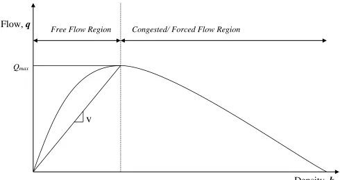
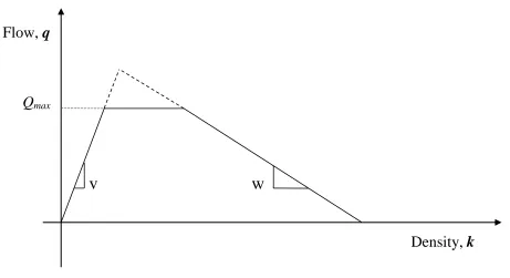
Though CTM can be applied to any flow-density relation (figure1a), a particular trapezoidal flow-density function is generally used (figure1b). According to the flow-density curve used for CTM, there is a constant free-flow speed (higher speed) at low densities and constant shockwave speed (always less than the free-flow speed) at high densities. Empirically it can be shown that the free-flow speed decreases mainly while the density approaches the flow capacity and otherwise it is fairly constant over a wide range of low densities.

CELL REPRESENTATION FOR A SINGLE LINK [Daganzo, 1994]: For CTM the single link is assumed to be divided into a number of cells of equal length. The length of each cell is the distance traversed in one tick of clock by a single vehicle travelling at free-flow speed. To define the characteristics of a cell,

 ni(t) : the number of vehicles in any cell i at time instant t

 Ni(t) : the maximum number of vehicles that can be present (holding capacity) in cell

i at time instant t

 Q i(t) : the maximum vehicle flow possible to cell i while clock ticks from t to t+1.

 Yi(t) : vehicles ready to enter cell I at time step t.

Ni(t) = (kj)x nl x L

where, kj is the jam density [veh/km-lane];

nl is the number of lanes in the cell;

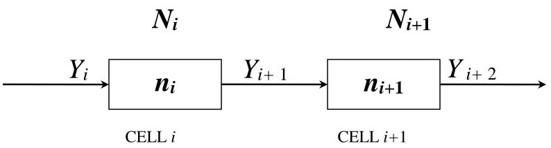
The whole CTM for a single link (figure 2) can be expressed by two equations: 1. The equation of state:

Yi+1(t) = min{ ni(t), Qmax,  [Ni+1(t)- ni+1(t)]} [3]

where,

Yi+1(t) is the inflow to cell i+1 at any instant t;

Qmax is the maximum number of vehicles that can enter cell i+1 at any single tick

of clock;

Ni+1(t) – ni+1(t) is the available space in cell i+1;

is the ratio of shockwave speed to free-flow speed (w/v);

This equation covers both the congested and uncongested situation. In the case of uncongested flow, the situation in the upstream cell i.e. the first term determines the flow; whereas in the congested situation downstream conditions i.e. the third term determines the flow. The middle term acts as the constraint in the case of bottlenecks.

2. The conservation equation:

ni(t+1) = ni(t) + Yi (t) - Yi+1(t) [4]

This equation updates the flow in consecutive cells at each time step. According to the equation the number of vehicles present in cell i at time instant t+1 is the number of vehicles present in the cell before the time step, plus the inflow to the cell minus the outflow from the cell during this time step.

If the cells are signalized (Lo, 1999a & b), then the maximum holding capacity Q i(t) of any

cell i varies as follows-

max if green phase

( )

0 if red phase

i

Q t

Q t

t  

  _

CELL REPRESENTATION FOR A NETWORK: A network consists of an ensemble of directed links and nodes. Each of the links can be modelled for CTM using the technique described for a single link. The only improvements are required while modelling the nodes attached with multiple links. Daganzo [1995b] suggested the allowed topologies (merges and diverges) in a network and their representation in CTM. For a signalized network Chang [1998] further developed these representations for ‘signalized merges’ and ‘turning lane diverges’ case. Here the network topologies used in the paper are discussed.

Merges are one the most important movements to be modelled while dealing with a network. According to Daganzo [1995b], there are three types of merge conditions possible.

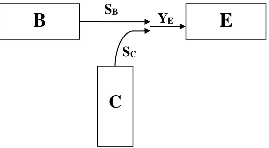
MERGES:

There can be three possible types of merging scenarios:

1. Forward: If flows from both the merging approaches (here, cells) depend on the conditions upstream (both approaches flowing freely).

2. Backward: If flows from both the merging approaches/cells depend on the conditions downstream (both approaches are congested).

3. Mixed: If the flow from one merging approach depends on downstream conditions while the other on upstream conditions (when the priority crowds out traffic on complementary approach)

Boundary conditions used here to get the CTM form are similar to those for two merging pipes carrying a compressible fluid. Figure 3 shows a ‘merge’ manoeuvre.

 





B B E C B E

Y t mid S R S p R [5a]

 





C C E B C E

Y t mid S R S p R [5b]

, _{E B C}

where, SB and SC are maximum possible outflow from the two sending cells B and C

respectively while RE is the maximum possible inflow to cell E; YB and YC are the emitting

flows from the cells B and C. p _B and p_C are the proportions of RE coming from the cells

and C respectively.

The equations 5(a) to 5(c) are the generalised form of equation 3 used for ‘merges’ in a

network. Using the equation 4 the flows can be updated.

Unsignalised and Signalised Merges: From figure 3, both the cells B and C flow into the cell

E. In case of both signalised and unsignalised junctions, the three equations 5(a) to 5(c) are to

be used. Only the constants p _B and p_C will be different for signalised and unsignalised

junctions. These constants are to be determined while designing any intersection which captures this kind of merging manoeuvre.

The set of equations 5(a, b & c) will remain in the same form for unsignalised junctions. Only it is to remember always thatp_Bp_B 1.

In the case of a signalised intersection, cell B and cell C don’t flow in the same time to cell E. Under these circumstances, where a maximum of one cell can flow at a time, the constants

B

p and p will be either 1 or 0. The set of equations 5(a, b & c) will simplify to, C

 

 

 





 

0, , 0;

, , 1;

B B

B B E B

Y t if p t

Y t min S R if p t

 

  [6]

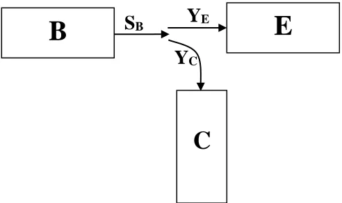
DIVERGES:

used here. As shown in figure 4, with this option, vehicles from a single cell (here cell B) can flow to two different destination cells (here, cell E and cell C) in two different directions. Considering that the turning proportions are known from beforehand, the inflow to each cell is,

 

 

C C B E E B

Y  S t Y  S t [7]

where, Y_C: the inflow to cell C

E

Y : the inflow to cell E

 

S t : the outflow from cell B at time instant t

and, _C& _Eare the proportions going to cells C and E respectively. As both cells C and E

are considered as destinations of the outflow from cell B, if any of them is unable to accommodate the allocated inflow then the entire outflow is restricted. This is to maintain FIFO (first in first out) principle. Hence,

 

 

 

 

E E E

C C C

n t Q t S T min

min Q t N t n t min Q t N t n t

           _{ }       [8]

2.

SEASONAL ARIMA MODEL:

A simple ARIMA model constitutes three parts, ‘AR’, i.e. autoregressive part; ‘I’, i.e. differencing part; ‘MA’, i.e. moving average part; ‘Differencing’ is essentially a tool to

The ‘first difference’ '

t

y

1

t t t

y

y y

In an ‘auto regressive’ process, each time-series observation ‘yt’ is defined in terms of its

predecessors, ‘ys’, for s < t, by the equation,

1 1 p l t t t l

y

y

Z







where, 1, 2,3,p are the coefficients of the auto regressive process of the order p.

A ‘moving average’ process is simply a finite linear filter applied to a white noise sequence

{Zt}, of the form

1

q

j

t t j

t

j

y

Z

Z

 



where, 1, 2,3,q are the coefficients of the moving average process of the order q.

Combining these three components and using the ‘backshift operator’, B, the equation representing an ARIMA (p, d, q) model is,

Z B y

B

B t t

d ) ( ) 1 )( ( 

   [1d]

where, Zt is a white noise sequence;

 is a polynomial of degree p, i.e. 2 3

2 3

1

( ) (1 .... p)

p

B B B B B

       and is a

polynomial of degree q, i.e. 2 3

1 2 3

( ) (1 .... q)

q

B B B B B

       . [1e]

In ARIMA (p,d,q), p denotes the order of the AR process, d denotes the order of differencing and q denotes the order of MA process.

Seasonality and ARIMA Process

[Fuller, 1996]

model the non-seasonal part (p, d, q) and the seasonal part (P, D, Q)s part are multiplied

together. The equation used for the multiplicative seasonal ARIMA model is as follows: B)BS)(1-B)d(1-BS)D yt= (B)(BS)Zt [1f]

where, have the same significance as described in the earlier section and  are their seasonal counterparts, S denotes the seasonality. The centred traffic data is used for ARIMA modelling using Box and Jenkins [Box and Jenkins, 1970] methodology. Following the three steps of this methodology, Identification, Estimation and Diagnostics checking a few seasonal ARIMA models are fitted.

3.

TRAFFIC NETWORK USED:

The traffic network used here for modelling using a combined CTM and time series forecasting approach is a part of the busy city centre of Dublin (figure 5). Considerable queue formation and congestion can be encountered in this site during the peak hours. The main thoroughfares are Tara Street and the Quays, which carry one-way traffic throughout. Two crossings of Tara Street with Pool beg Street and the Quays are considered here. Two un-signalised side streets from the quays are also considered within the network. All of the crossroads carry one-way traffic as well as the main streets. Ireland has a left-hand drive system with no protected turning movements in this site. Junction TCS183 and TCS184 has two phased signals, but the two downstream junctions have multi-phased (>2) signal plans.

3.1 DATA COLLECTION FOR CTM MODELLING:

control) are obtained from the SCATS database as well. Other required constants for the CTM model are,

 Free flow speed [60 dataset]  Saturation Flow [40 dataset]  Shockwave speed [30 dataset]

Other than these for the turning movement (which is not obtained from the loop-detectors), 16sets of data from each lane, used for both through and turning movements, are collected. Using this manually counted data and the loop detector volumes, turning ratios and the merge ratios are calculated.

3.2 CTM REPRESENTATION AND CALIBRATION OF THE NETWORK:

The links are divided into equal length cells (whose length is governed by the free flow speed and the space discritisation criteria). The possible movement in and out of the cell are represented by directional arrows. Figure 6 shows a figurative representation of the network. Turing movements along with merges and diverges are modelled as can be seen from figure 6. The capacity of each approach or more precisely each lane is decided judging the site conditions and past traffic demands.

4.

TIME-SERIES MODELLING OF LOOP OBSERVATIONS

are obtained from the inductive loops of those streets. The data used for modelling were recorded from 16th _{May 2005 early morning to 30}th _{June 2005 early morning, excluding}

the weekends and bank holidays. 96 observations are obtained in each day. The total number of observations is 2592 are obtained from each data source. The data show definite seasonality in pattern over a period of 24 hours. This leads to the idea of fitting a seasonal time-series model. As this site is the same as (or very similar) to that of the paper by Ghosh et al.[2005], more or less the same seasonal ARIMA models are used in modelling the observations. All the seasonal ARIMA models fitted to each origin traffic demand data are given in table 2.

5.

COMPARISON OF CTM RESULTS WITH REAL TIME FLOW:

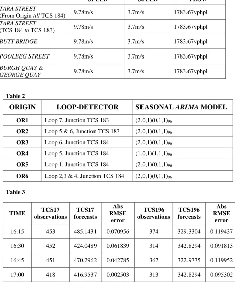
Although it was expected that there would be manual errors during data collection, most of the predictions were within 10% of the actual observations. The mean absolute percentage of the 1 hour prediction data set (table 3) is only 4.4% in Junction TCS 17 and 10.6% in TCS 196. The error has two parts; one is due to CTM simulations and one related to using the time-series forecasts as input traffic demand instead of real observations.

was not exactly fixed and the phase times were varying in the order of ½ seconds 0.5 seconds??. But as the pedestrian phases are not recorded by the SCATS system, the average fixed cycles of 120 second were to be assumed. Due to this average cycle time over 4:00pm to 5:00pm of 30th, June, 2005 are used, instead of an exact signal time plan and accurate cycle lengths as used for Junction TCS 183. This error in the order of 2/3 seconds may be attributed to a considerable percentage to the final error values.

6.

CONCLUSION:

The empirical based time-series forecasting technique is integrated with the theoretical ‘Cell-Transmission Model’ (CTM) to effectively simulate the traffic demand at two

REFERENCES:

1. Van Arem, B., Kirby, H.R., Van Der Vlist, M.J.M. and Whittaker, J.C. (1997), Recent advances and applications in the field of short-term traffic forecasting, International Journal of Forecasting, Vol. 13, pp. 1-12.

2. Ahmed, M. and Cook, A. (1982), Analysis of Freeway Traffic Time Series Data by Using Box-Jenkins Techniques. In Transportation Research Record: Journal of the Transportation Research Board, No. 722, TRB, National Research Council, Washington, D.C., pp. 1-9.

3. Lee, S. and D. Fambro. Application of The subset ARIMA Model for Short-Term Freeway Traffic Volume Forecasting. Transportation Research Record: Journal of the Transportation Research Board, No. 1678, TRB, National Research Council, Washington D. C., 1999, pp. 179-188.

4. Williams, B.M. and Hoel, L.A. (2003), Modeling and Forecasting Vehicular Traffic Flow as a Seasonal ARIMA Process: Theoretical Basis and Empirical Results. Journal of Transportation Engineering ASCE, Vol. 129(6), pp. 664-672. 5. Ghosh, B., Basu, B. and O’Mahony, M.M. (2005), Time-series modeling for

forecasting vehicular traffic flow in Dublin, Presented at the 78th Annual Meeting of Transportation Research Board, Washington, D. C., 2005.

6. Daganzo, C.F. (1994), The Cell Transmission Model: A Dynamic Representation Of Highway Traffic Consistent with the Hydrodynamic Theory. Transportation Research B, Vol.28, pp. 269-287.

7. Daganzo, C.F. (1995), The Cell Transmission Model, Part II: Network Traffic. Transportation Research B, Vol.29, pp. 79-93.

8. Daganzo, C.F. (1995) Finite Difference Approximation Of The Kinematic Wave Model Of Traffic Flow. Transportation Research B, Vol.29, 261-276.

9. Lo, H., Chang, E. and Chan, Y.C. (2001a), Dynamic Network Traffic Control. Transportation Research A, Vol.35, pp. 721-744.

10.Lo, H. (2001b), A Cell-Based Traffic Control Formulation: Strategies And Benfits Of Dynamic Timing Plans. Transportation Science, Vol.35 (2), pp. 148-164.

12.Richards, P.I. (1956) Shockwaves on the Highway. Operations Research, Vol.4, 42-51.

List of Tables:

1. The Road specifications 2. The Traffic Demand Models 3. The Error Estimates

List of Figures:

1(a). The Fundamental Flow-density Diagram 1(a). The Flow Density Relationship Used in CTM 2. The Basic CTM Model for Single Link with Two Cells 3. A Signalised Merge

4. A Diverge Manoeuvre

Table 1

ROAD NAME FREE FLOW

SPEED SHOCKWAVE SPEED SATURATION FLOW TARA STREET

(From Origin till TCS 184) 9.78m/s 3.7m/s 1783.67vphpl TARA STREET

(TCS 184 to TCS 183) 9.78m/s 3.7m/s 1783.67vphpl BUTT BRIDGE 9.78m/s 3.7m/s 1783.67vphpl

POOLBEG STREET 9.78m/s 3.7m/s 1783.67vphpl BURGH QUAY &

GEORGE QUAY 9.78m/s 3.7m/s 1783.67vphpl

Table 2

ORIGIN

LOOP-DETECTOR

SEASONAL ARIMA MODEL

OR1 Loop 7, Junction TCS 183 (2,0,1)(0,1,1)96

OR2 Loop 5 & 6, Junction TCS 183 (2,0,1)(0,1,1)96

OR3 Loop 6, Junction TCS 184 (2,0,1)(0,1,1)96

OR4 Loop 5, Junction TCS 184 (1,0,1)(1,1,1)96

OR5 Loop 1, Junction TCS 184 (2,0,1)(0,1,1)96

OR6 Loop 2,3 & 4, Junction TCS 184 (2,0,1)(0,1,1)96

Table 3

TIME TCS17

Table 4

Junction Street Name Phase Offset Green

Effective

Red Effective

TCS 183

Burgh Quay & George Quay B 72sec 45sec 75sec

TCS 184

Figure 1a: The Fundamental Flow-density Diagram Qmax

Flow,

q

Density,

k

v

Figure 1b: The Flow Density Relationship Used in CTM

Q

v

w

Figure 2: The Basic CTM Model for Single Link with Two Cells Ref: Lo & Chan (2001a)

n

n

CELL i CELL i+1

N

N

Figure 3: A Signalised Merge Ref: Lo & Chan (2001a)

B

E

C

S

S

Figure 4: A Diverge Manoeuvre Ref: Lo & Chan (2001a)

B

E

C

S

Y

Figure 6: The Cell Representation of the Network

TARA STREET

25 26

27 31 34 30

32 33

28 29 15 16 17 21 24 20

22 23

19 18 13 14 11 12 1 3 5 6

7 4 2 8

9 10

35 36

37 42 41 40 38 39 43 97 96 95 93 94 98 92 91 50 51 52 53 54 55 56

57 49 48 47 46 45 44