A Comparison of some Negotiation Algorithms using a Tournament Based Approach

Tournament-Based Approach

Peter Henderson, Stephen Crouch, Robert John Walters, and Qinglai Ni

Declarative Systems and Software Engineering, Department of Electronics and Computer Science,

University of Southampton, Southampton, UK, SO17 1BJ

{ph, stc, rjw1, qn}@ecs.soton.ac.uk

Abstract. This paper provides some results and analysis of several negotiation algorithms. We have used a tournament-based approach to evaluation and applied this within a community of Buyers and Sellers in a simulated car hire scenario. An automated negotiation environment has been developed and the various negotiation algorithms made to compete against each other. In a single tournament, each algorithm was used as both a Buyer-negotiator and a Seller-negotiator. Each negotiating algorithm accommodates the parameters for negotiation as a set of desirable goals, represented as examples of product specifications. It was the task of each negotiating algorithm to get the best deal possible from every one of their opposites (i.e. Buyer versus Seller) in the sense of being close to the examples they were given as goals. One algorithm proved to be superior to the others against which it was made to compete.

1 Introduction

A significant problem in distributed e-commerce applications is the choice of algorithm used to carry out automated negotiation on behalf of a client [3], [4], [6], [7], [8], [12]. Even very simple algorithms can have behaviour which is acceptable in a restricted scenario but which might be unpredictable in a more liberal environment. In order to gain some confidence in algorithms we were planning to deploy, we decided to establish a simulation environment in which they could be evaluated.

One of the many interesting aspects of the work was that the algorithm that emerged victorious against all the others was incredibly simple. Tit-For-Tat simply cooperated with its opponent on the first round, and from then on just reciprocated whatever its opponent did on the previous round. Surprisingly, this algorithm accumulated more rewards than the others, although it would never actually win a complete game. It won because it encouraged high scoring games with its opponents, and although it was always either drawn with or beaten, it subsequently attained the highest score overall (see [2]).

Three characteristics formed the basis for its success: it never was the first to defect, it didn't hold grudges, but it was retaliatory. Cooperate with it, and you both do well. Defect against it and it does the same. We wondered if a similar result might hold where participants were engaged in negotiation. We have chosen to build a tournament that pits algorithms against each other, which, although simple, are of the sort that are actually used in commercial scenarios.

At an abstract level, similarities may be identified between the tournament presented in this paper and the tournament conducted by Axelrod. However, there are some very notable differences, since this experiment deals with interaction on a far more detailed, and therefore semantically rich, level.

Firstly, the scoring system has to be more comp lex. In negotiation, often there is no absolute notion of cooperation and defection as in the Prisoner's Dilemma. For example, what one Seller views as defection by a Buyer is not always what another Seller would view as defection. The existence of this perceptual grey area means a more detailed scoring system to ensure consistency across scores was required.

Secondly, the algorithms in this tournament are each given a set of negotiation goals, in the form of desired product specifications. Interpreting and reasoning about these goals in some way is an issue that has to be dealt with by the algorithms.

Thirdly, in this tournament, all algorithms face each other, including instances of themselves, as Buyers versus Sellers.

Previously we have looked at architectures for e -commerce systems [10], [11], [12] and been interested in how federations of applications co-operate, particularly when new applications can join the federation at any time. Networks of e-commerce negotiation algorithms have exactly this property and have become a test case for us.

Chapter 2 describes the nature and context of the experiment. The car hire negotiation scenario is discussed in Sect. 2.1 and the negotiation environment is outlined in Sect. 2.2. Sect. 2.3 details the generic behaviour of the negotiators, and Sect. 2.4 introduces the use of example specifications as goals, and describes the two sets of examples used for the experiments.

Chapter 3 provides a behavioural description and brief discussion of each of the seven algorithms.

2 The Experiment

2.1 The Car Hire Scenario

The chosen scenario for the negotiation tournament was car hire. If we consider a single Buyer and Seller pair in the tournament, a Buyer's objective is to secure the best deal possible for hiring a car, with respect to a given set of car specifications. The Buyer has a set of examples of deals they would accept. Each entry in this set consists of four attribute name and value pairs for the following attributes:

− Days the length of time we wish to hire the car

− Price the price we would like to pay

− Features some linear, quantified grade of features (e.g. air conditioning, electric windows), higher number represents more features

− Class the desired size of the car, higher number represents larger car

A set of examples consists of car specifications, each representing an acceptable outcome of negotiation. The Seller also has a set of examples, representing the cars they wish to hire out, reflecting their stock constraints.

Specifying negotiation criteria as examples provides an abstract yet flexible method of stating a negotiator's desires, although the potential exists for ambiguity between these example criteria. There is not always a clear correlation between these examples, and interpreting them in the context of the negotiation process and using this understanding to guide actions are behavioural tasks of the negotiator [13].

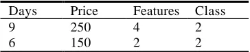
Table 1. A set of examples to be used as Buyer goals

Days Price Features Class

9 250 4 2

6 150 2 2

Consider the examples in Table 1. If these are examples used by a Buyer, then we see that they are after a particular class of car and want about 9 days of hire. They are prepared to compromise on days (and features) but only for a significant saving in cost. If the Buyer using these examples receives an offer that is close to one of these examples, they would be inclined to accept it. If they have to make a counter offer, they will construct one using an algorithm which takes into account offers they have received and which attempts to stay close to these examples. It is algorithms of this sort (for Sellers as well as Buyers) that we wish to evaluate.

2.2 The Negotiation Environment

A negotiation environment was developed within which multiple automated negotiators could compete. Two applications form this environment:

− Negotiator given a set of negotiation examples and environment parameters (round cut-off, opponent negotiator identities) and is responsible for conducting negotiation

The environment allowed for a configurable number of Buyer and Seller negotiators to be instantiated for a single tournament, each with their own algorithm for conducting negotiation, and each with a set of either Buyer or Seller examples. These examples provide a set of acceptable goals for each negotiator. Once the scenario has been initiated, it remains fixed. Therefore, it is not possible to simulate situations where a negotiator switches its behaviour to that of other algorithms during a negotiation. However, this can be achieved by modelling multiple behaviours within a single algorithm. In which case, the algorithm can switch between them when it sees fit.

The negotiation environment was designed and implemented such that the process of inserting a new algorithm into the tournament and allowing it to compete with the others was simple and rapid. This process was as follows:

− Description the algorithm is described in pseudocode

− Translation & Compilation this pseudocode is translated into Visual Basic and compiled into an executable

− Add to Supervisor List the name of the algorithm is added to the Supervisor's list of available algorithms

To a great extent, by careful design of the pseudocode language, the translation to Visual Basic is mechanistic.

In a typical tournament, a Buyer's target is to secure one car from each Seller, whilst the Seller's target is to sell one car to each Buyer. If we adopt a global view of all negotiations, we essentially observe a series of pair-wise negotiations between each possible Buyer/Seller/algorithm permutation, with successful negotiations resulting in the exchange of a car from a Seller to a Buyer. In other words, after a tournament is complete, every Buyer will have negotiated once with every Seller, and vice-versa, and every algorithm in a tournament will be represented as both a Buyer and Seller.

In a typical tournament, although all negotiations between Buyers and Sellers are handled concurrently, the actions of each Buyer do not affect other Buyers, and the same is true for Sellers. This is because each Seller potentially has one car to hire out to each Buyer. However, if we give each Seller less cars than there are Buyers, the actions of a Buyer have possible ramifications for other Buyers, since those which typically take more time in reaching agreement may not secure a car. This makes it possible for us to run a tournament with the added element of competition for resources, where an algorithm's efficiency contributes to success. This has not been done in the experiments reported here.

To measure the success of a negotiator following a tournament, a simple scoring system was devised and applied to each outcome of each negotiation for a negotiator. Only two possible outcomes of negotiation between a Buyer and a Seller exist:

manages to secure with another, either by accepting an offer themselves, or having one of their offers accepted, a measure of 'distance' between that offer and their given set of examples provides us with a base score. Therefore, accepting an offer (or having it accepted) that perfectly matches one of their examples will get them the best score possible. An acceptance facilitates one car being passed from the Seller to the Buyer as a resource.

− Quit Determined and imposed by the negotiation environment, if a Buyer-Seller pair is still negotiating after a given number of rounds, their negotiations are terminated and they each receive a score of zero. In addition, the Seller does not sell a car, and the Buyer does not receive one. This outcome represents the penalty for not reaching an agreement, and therefore provides an incentive for each algorithm to reach agreement quickly. However, they are not told prior to the tournament how many rounds they are not allowed to exceed. Similar in motivation to the Axelrod tournament, algorithms cannot therefore attempt to do better than their negotiation opponents by using their knowledge of the maximum number of rounds to try to take advantage [5].

It is in the best interests of a negotiator's algorithm to reach agreement with their opposites under any circumstances, and to do so quickly. It is intentional that securing a bad deal quickly and receiving a low score is a better outcome than not securing a deal and receiving a zero score. Another approach would have been to offer algorithms the choice of quitting negotiations themselves instead of making another offer, and many scoring methods could have been employed. However, it was decided that the main objective of the tournament is to ascertain how well each algorithm can negotiate with each other, not how well strategically they can quit negotiations. An algorithm that knows when to quit against another, perhaps to attain the best payoff, does not tell us very much about how effectively it negotiates. However, such an algorithm can be simulated. It would simply repeat its final (rejected) offer until such time as the supervisor intervened.

The algorithm used for calculating the distance between an accepted offer and a set of examples was straightforward. For each attribute in an offer, a minimum and a maximum allowed value are imposed. No penalty is awarded for going outside of these ranges, but any offending attributes are constrained within those ranges. These range values are accessible by an algorithm, and this mechanism therefore provides a sanity check against offers that may inhibit the operation of the system, but more importantly these range values provide a scope for scoring algorithms. The scoring function takes an accepted offer and an example and returns an inverse measure of 'distance' between the two, as a value between 0 and 1. i.e. the higher the score, the closer the offer to the given example.

2.3 Negotiation Behaviour

The negotiation process between a Buyer and Seller consists of a series of offers and counter-offers being made until an agreement is reached, with a single offer consisting of Days, Price, Features and Class attribute and value pairs. Of course, during negotiation it may prove impossible for a Buyer to acquire exactly what they want from the Seller, or vice versa, so each negotiator must be able to compromise on certain attributes in order for negotiation to be successful. However, it is obvious that it is not in the best interests of each negotiator to over-compromise, simply because this could mean they secure a deal which does not match with their desired criteria. The manner and degree in which a negotiator deviates from those criteria is dictated by the negotiation strategy they employ.

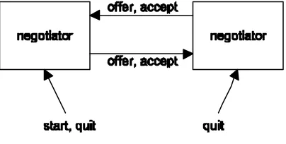
Figure 1 shows the messages that will flow between two negotiators, one configured as a Buyer and one as a Seller. The supervisor will tell one or other (we will always use the Buyer) to start.

Fig. 1. The negotiation scenario

Offers will alternate according to a predefined behaviour specified in the negotiator.

Pseudocode representation of the behaviour of the negotiator

on receive start from supervisor { compute initial offer;

send offer to partner; }

on receive offer from partner { evaluate offer;

if (offer is acceptable) { send accept to partner; exit;

} else {

compute new offer; send offer to partner; }

}

Eventually either one of the negotiators accepts or the supervisor tells both to quit. Each negotiator is initialised with this behaviour, and is told that it is buying or selling against a set of examples with which it has been furnished. Each algorithm will take a different approach to implementing one or other of the basic actions:

− compute initial offer,

− evaluate offer,

− compute new offer.

Before we go into further detail of the actual algorithms that we use, we need to say a little more about the examples.

2.4 The Examples

In order to understand how and to what extent the examples contribute to the results, two very simple sets were used, each with different qualities. Set one is shown in Table 2 and Table 3.

Table 2. Buyer example set 1

Days Price Features Class

9 200 4 2

8 190 3 2

Table 3. Seller example set 1

Days Price Features Class

7 300 3 2

4 150 2 1

Essentially, for the Buyer and the Seller, each of their examples is roughly consistent with each other, and appears quite rational. Comparing the Seller's examples with the Buyer's examples shows the Buyer would take one less day and a slightly less featured car for $10 less, whilst the Seller would like to hire out a less featured, smaller car for half the price.

Set two is shown in Table 4 and Table 5.

Table 4. Buyer example set 2

Days Price Features Class

10 200 3 4

8 140 2 3

Table 5. Seller example set 2

Days Price Features Class

8 260 2 2

These examples were designed to be less consistent and more difficult to reason about. If we consider the Buyer's second example, the Buyer wishes to hire a big, low features car for 8 days at $140, yet would be willing to pay $60 more for two extra days and a slightly better featured, larger car. However, the Seller's second example is $170 for a small car with low features for 6 days. His first however, is a great deal more for only two extra days and a moderately sized car. It should be noted that the first set of examples appears to provide a little more room for 'negotiation manoeuvring' than the second set. In other words, the Buyer and Seller negotiation criteria are further apart in the first set than the second set. Giving the algorithms a smaller bargaining arena gives us the opportunity to observe how well they perform under such tight circumstances.

Although we have run experiments with larger example sets, the results are essentially as those reported here. The smaller example sets make clearer what is going on.

3 The Algorithms

Seven algorithms were developed and submitted to compete in the tournament. Each algorithm had to address the following three questions:

− What constitutes an initial offer if the algorithm is a Buyer?

− Under what circumstances is an offer accepted?

− If the most recently received offer is not accepted, how is a counter-offer formulated?

In these terms, let us describe the seven algorithms that we compared.

The first two algorithms, Random and JustAccept, were trivial. These algorithms were included purely for comparison with other algorithms. Obviously, any algorithm should always do better than Random or JustAccept, so these two algorithms provide a 'comparison bar' for the lowest level of performance. Interestingly, we discovered that some algorithms were not able to beat either of these trivial choices.

3.1 Random

Random simply produced random offers, by picking a random number between the minimum and maximum ranges for each attribute. Each time an offer was received, random would have a 10% chance of accepting it.

− Compute Initial Offer: choose arbitrary values for each attribute within permitted ranges

− Evaluate Offer: accept probabilistically (for these experiments, with 10% chance)

3.2 JustAccept

JustAccept simply accepted the first offer it received, and if it was a Buyer, its first offer was simply its first example.

− Compute Initial Offer: choose first example

− Evaluate Offer: always accept

− Compute New Offer: never happens

3.3 AgreeRandomAttribute

This algorithm only attempts to negotiate with respect to its first example, which forms its first offer if it is a Buyer. After receiving an offer, it uses its first examp le as an offer template. Into this offer template it randomly substitutes an attribute value from the opponent's offer. This offer template forms the new offer. It will accept an offer if it only has one attribute different from any one of its examples.

− Compute Initial Offer: choose first example

− Evaluate Offer: accept if agreement in all but at most one attribute

− Compute New Offer: alter one attribute to equal value received from opponent

3.4 AgreeProgressive

AgreeProgressive was a more accommodating, and more sophisticated, version of AgreeRandomAttribute. It utilises a matrix that acts as a mask for merging an example and an offer to form a new offer. The merging process is simple: the best matching example to the last received offer is used as the temp late, and the matrix decides which attribute values in the template to substitute. In the first four rounds, the algorithm will accept an offer with only one different attribute to one of its examples. Otherwise, on a per-round basis, it cycles through each attribute, substituting the appropriate attribute in the closest matching example for the corresponding attribute in the last received offer. The closest matching example is the one with the least number of different attributes from the last received offer.

In the next 6 rounds, the number of attributes to substitute is increased to two. Every possible permutation of two attributes is attempted. A received offer is accepted if it differs from one of its examples by only two attributes.

In rounds 11 to 14, all possible permutations of three attributes are attempted, and offers are accepted if different from an example by only three attributes. When the algorithm reaches round 15, it will accept whatever offer is sent by the opponent.

− Compute Initial Offer: choose first example

− Evaluate Offer: accept if agreement in all but at most one (two, three, ...) attributes

3.5 Tit-For-Tat

This algorithm represents a simple interpretation of Axelrod's Tit-For-Tat in the context of negotiation. It replicates on an attribute-attribute basis the inverse behaviour of the opponent. This behaviour is determined by simply comparing the opponent's most recent offer with the one received before that. e.g. if the opponent (as a Seller) deducts $10 off the price, the Buyer as Tit -For-Tat will add $10. Until Tit-For-Tat has two offers to compare, it initially cooperates by adding 10% onto its previous offer.

− Compute Initial Offer: choose first example

− Evaluate Offer: accept if offer within a margin of one example

− Compute New Offer: for each attribute, reflect opponent's behaviour by moving the same degree in the opposite direction: if opponent closes gap, then close gap. If opponent opens gap, then open gap

3.6 Retreat

This algorithm begins by offering the first example. As negotiation progresses, it then proceeds to 'back away' from this example in the opposite direction of the opponent's last received offer. If the opponent's offer is close to this example, it accepts the offer.

− Compute Initial Offer: choose first example

− Evaluate Offer: accept if agreement within a margin

− Compute New Offer: for each attribute, regardless of whether opponent opens or closes gap, open gap by 10%

3.7 TestAlgorithm

This algorithm employed a numerical method to dictate its offers, and to determine whether to accept an opponent's offer. This is an attempt to emulate the kind of rational algorithm which is often deployed in practice, where some quantitative knowledge of the domain is used to refine its decision making process.

− Compute Initial Offer: choose first example

− Evaluate Offer: accept if agreement within a margin

− Compute New Offer: numerical method of moving within region of disagreement with opponent

4 Results

not entirely as we would have expected. We did not predict that AgreeProgressive would do as well as both Buyer and Seller. Nor did we expect the rational TestAlgorithm to do so badly as a Seller.

Table 6. Buyers using the first example set

Negotiator Algorithm Resource Used Score Final Score

Buyer4 AgreeProgressive 1 0.937 0.937

Buyer5 Tit-For-Tat 1 0.901 0.901

Buyer1 TestAlgorithm 1 0.898 0.898

Buyer7 JustAccept 1 0.883 0.883

Buyer2 Random 0.986 0.799 0.788

Buyer6 Retreat 0.857 0.786 0.674

Buyer3 AgreeRandomOne 0.7 0.673 0.471

Table 7. Sellers using the first example set

Negotiator Algorithm Resource Used Score Final Score

Seller4 AgreeProgressive 1 0.948 0.948

Seller6 Retreat 0.993 0.920 0.913

Seller7 JustAccept 1 0.860 0.861

Seller2 Random 0.993 0.781 0.776

Seller3 AgreeRandomOne 0.843 0.819 0.691

Seller5 Tit-For-Tat 0.857 0.794 0.680

Seller1 TestAlgorithm 0.857 0.737 0.631

Table 8. Buyers using the second example set

Negotiator Algorithm Resource Used Score Final Score

Buyer4 AgreeProgressive 1 0.860 0.860

Buyer7 JustAccept 1 0.823 0.823

Buyer1 TestAlgorithm 1 0.816 0.816

Buyer2 Random 0.993 0.748 0.742

Buyer5 Tit-For-Tat 0.843 0.757 0.638

Buyer6 Retreat 0.571 0.511 0.292

Buyer3 AgreeRandomOne 0.457 0.441 0.202

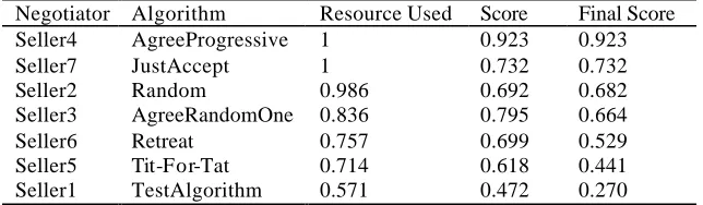
Table 9. Sellers using the second example set

Negotiator Algorithm Resource Used Score Final Score

Seller4 AgreeProgressive 1 0.923 0.923

Seller7 JustAccept 1 0.732 0.732

Seller2 Random 0.986 0.692 0.682

Seller3 AgreeRandomOne 0.836 0.795 0.664

Seller6 Retreat 0.757 0.699 0.529

Seller5 Tit-For-Tat 0.714 0.618 0.441

Some algorithms never reach agreement, even though doing so entails such a severe penalty. The reasons for this are threefold: firstly, the algorithms do not know how many rounds of negotiation they are allowed. If they did, they could simply accept the last offer made by their opponents before the cut-off. Secondly, each negotiator faces the simple dilemma of whether to accept the other negotiator's latest offer, or to make another offer. Because they have no global view of how negotiations will turn out, they cannot know at any point during negotiations whether the most recent offer received is the best they will ever get. Thirdly, the negotiation behaviour that emerges as a result of the inherent nature of each algorithm, when faced with the other, may guarantee they never reach agreement. Retreat, for example, could never reach agreement with AgreeRandomAttribute if each of their examples were sufficiently far apart.

AgreeProgressive was more successful than we expected. The behaviour reported here was repeated in other experiments, including for larger example sets. Most importantly, it is the only algorithm that will always reach agreement as long as the negotiation cut-off is at least 15 rounds (for 4 attributes). At round 15 it eventually agrees with whatever the opponent is then offering. As long as this is the cas e, this ensures that the algorithm is never penalised for not reaching agreement early enough. Secondly, the nature of the algorithm means that it gradually alters its negotiation strategy from initially very stubborn (only agreeing to one attribute), to very conciliatory (agreeing with all four attributes, and therefore accepting the offer). Every possible permutation of offer agreement within these two extremes is presented to the opponent, and therefore the likelihood that an offer will be accepted incre ases with every iteration. Thirdly, because the algorithm is initially very stubborn, this allows the algorithm to take advantage of any concessions that may be made by the opponent in the earlier stages of negotiation, before it begins to compromise on a greater scale. This can be seen with TestAlgorithm. Unlike algorithms such as Retreat and TestAlgorithm, AgreeProgressive does not waste time making ‘bluff’ offers. It immediately attempts to find a formula for mutual agreement. Tournament cut-off permitting, this will always be the case.

The relative success of JustAccept is a consequence of the nature of the other algorithms and the structure of the tournament. JustAccept does well because it always reaches a deal and because the opponents are behaving reasonably in that their offers are realistic. When JustAccept is acting as a Buyer, this is a close approximation to real life, where goods on sale are offered at a fair price and Buyers just accept that. It doesn't do quite as well as a Seller, but even there its behaviour is reasonable because Buyers open with reasonable bids. This algorithm is obviously open to exploitation, but the tournament has been structured to prevent this. Nonetheless, JustAccept has performed its role as a benchmark for calibrating the performance of others. The only algorithm to perform consistently better than JustAccept was AgreeProgressive, assuming the number of negotiation rounds was at least 15.

The results presented here are typical. In other experiments, with different example sets and identical environment configurations, the ranking of the algorithms remains similar to the results displayed here. AgreeProgressive consistently does exceptionally well against the others, as a Buyer or Seller, as long as the round cut-off is at least 15 rounds. In its worst test it came third as a Buyer, but the tournament leader, Retreat in this case, was only ahead by a score of 0.006. Conversely, AgreeRandomOne performs very badly, always last in the rankings. The order of the middle rankings as shown in this paper is also representative. Of course, with some example sets, other algorithms do better than others, but in general big differences in the ranking are uncommon.

5 Conclusions

We have described a series of experiments that have allowed us to compare various negotiating algorithms. Following Axelrod we have taken the view that an algorithm is best if it does well against a range of opponents. Although negotiation is a more complex behaviour to describe (and hence to measure) than simple collaboration, we have arrived at a similar result to Axelrod. One algorithm has performed better than expected, consistently doing well against a range of opponents. The algorithm is not the simplest in our set, nor is it the one we expected to be best. These are observations we have explained, to some extent. Further experiments which we plan, with these algorithms and with new algorithms, will lead, we hope to a greater understanding of negotiated agreement in an e-commerce context.

References

1. Axelrod, R.: The Evolution of Co-operation. Basic Books Inc., New York (1984) 2. Axelrod, R.: The Complexity of Cooperation. Basic Books Inc., New York (1997) 3. Burg, B.: Agents in the World of Active Web Services. To be published in Springer

4. Bichler, M., Segev, A., Zhao, J.L.: Component-Based E-Commerce: Assessment of Current Practices and Future Directions. ACM Sigmod Record: Special Section on Electronics Commerce, Vol. 27, No. 4 (1998) 7–14

5. Binmore, K., Vulkan, N.: Applying Game Theory to Automated Negotiation. Netonomics, Jan. 99, see http://www.worcester.ox.ac.uk/fellows/vulkan (1999)

6. Cranor, L.F., Resnick, P.: Protocols for Automated Negotiations with Buyer Anonymity and Seller Reputations. Telecommunications Policy Research Conference (TPRC 97), see

http://www.si.umich.edu/~presnick (1997)

7. Farhoodi, F., Fingar, P.: Developing Enterprise Systems with Intelligent Agent Technology. Distributed Object Computing, Object Management Group (1997)

8. Fingar, P., Kumar, H., Sharma, T.: Enterprise E-Commerce. 1st edn. Meghan-Kiffer Press, Tampa FL (2000)

9. Fogel, D.B.: Applying Fogel and Burgin’s Competitive Goal-Seeking through Evolutionary Programming to Coordination. Trust and Bargaining Games. Proceedings of the 2000 Congress on Evolutionary Computation (CEC 2000), IEEE Press Piscataway NJ (2000) 1210–1216

10. Henderson, P.: Laws for Dynamic Systems. Proceedings of the Fifth International Conference on Software Reuse (ICSR 98), IEEE Computer Society Press, (1998) 330– 336

11. Henderson, P., Walters, R.J.: Behavioural Analysis of Component-Based Systems. Information and Software Technology, Vol. 43, No. 3 (2001) 161–169

12. Henderson, P.: Asset Mapping - Developing Inter-enterprise Solutions from Legacy Components. In: Systems Engineering for Business Process Change - New Directions, Springer-Verlag UK, (2002) 1–12 see http://www.ecs.soton.ac.uk/~ph/papers