Discretion and cyclicality in Irish budgetary management 1969 2003

Discretion and Cyclicality in

Irish Budgetary Management 1969-2003

COLIN HUNT* Trinity College Dublin

Abstract: This paper addresses the topic of cyclicality and discretion in Irish fiscal policy. In particular, we show that the level and nature of cyclicality varies across different expenditure components and we introduce a new definition of feasible discretion to take account of political imperatives in budgetary management. We find that overall government expenditure is acyclical and is most heavily influenced by a fiscal parsimony objective. Automatic stabilisers are efficiently counter-cyclical, feasible discretionary government consumption growth is orthogonal to economic fundamentals while feasible discretionary investment growth is strongly pro-cyclical. Using official growth forecasts, we show that feasible discretionary investment growth is deliberately pro-cyclical.

I INTRODUCTION

I

particularly in the advent and aftermath of membership of Economic and Monetary Union. A growing emphasis on budgetary management is something of a global phenomenon with dissent about the conduct of monetary policy fading as a general consensus emerges in favour of monetary stability. Taylor (2000) points out that the environment in which discretionary counter-cyclical

295

fiscal policy can be considered has fundamentally changed on the back of two factors: monetary policy has become more transparent and more reactive to changes in both inflation and output; and the emergence of new normative macroeconomics with an emphasis on evaluating policy rules.

Ireland is an interesting subject for study as fiscal outturns were wildly volatile over the course of the past three decades. Given the health of the public finances since the mid-1990s, the fiscal policy decision-making process is unlikely to have been distorted by pressure arising from the Maastricht criteria and, subsequently, the Stability and Growth Pact.

The existing body of work will be augmented by an analysis of the interaction between cyclicality, political choices and decomposed government expenditure for Ireland over the course of the 1969-2003 period. This paper highlights the cyclicalities of Irish government consumption, current transfers and investment adjusted to take account of both legal obligations and political imperatives and also examines the efficiency of automatic stabilisers. Attention is paid to the rank of government investment spending within the budgetary-formation process.

II THEORETICAL BACKDROP

The neo-classical view that government spending’s share of GDP should behave counter-cyclically is intuitively appealing given that pro-cyclical responses of fiscal policy exacerbate underlying fluctuations in consumption and output. Traditional Keynesian analysis suggests that fiscal policy should be counter-cyclical with government increasing spending and reducing taxes during recessionary periods and adopting an opposite stance during upturns. Under such a policy, there would be a positive correlation between tax rates and output while the correlation between government spending and output would be negative.

Further underpinning is provided by Eichenbaum (1997) who claims that there is widespread agreement that counter-cyclical discretionary fiscal policy is neither desirable nor politically feasible. Such a claim should be regarded as something of an overstatement particularly in light of the aggressive counter-cyclicality of US fiscal policy during the most recent economic downturn. Indeed, given concerns about the potential inertia of monetary policy at times when nominal interest rates are low and given the real threat of deflation, the desirability and feasibility of counter-cyclical discretionary fiscal policy have been enhanced in the early years of this decade. Recent experiences also erode Eichenbaum’s observation that practical debates about stabilisation policy revolve almost exclusively around monetary policy.

2.1 Previous Empirics

In conflict with the theoretical foundations, a number of empirical studies have found that pro-cyclicality is, in fact, commonplace. Gavin and Perotti (1997), in a study of Latin American countries, show that fiscal policy is pro-cyclical and suggest that this phenomenon is due to the difficulties experienced by developing nations in accessing international credit flows during cyclical downturns. Their work was supported by Talvi and Vegh (2000) who suggest that pro-cyclical fiscal policy is so pervasive in the world economy that it should arguably be regarded as the rule rather than the exception. In a sample of 56 countries, they show that fiscal policy is acyclical among G7 countries, cyclical among non-G7 industrial countries and strongly pro-cyclical among developing economies.

In explaining this puzzle, they introduce a political distortion into the standard optimal fiscal policy model which encapsulates the pressures which arise to increase public spending on the back of budget surpluses. Tornell and Lane (1999) refer to this phenomenon as the voracity effect where powerful groups attempt, in response to a positive revenue shock, to grab a greater share of national wealth. With this political adjustment, Talvi and Vegh suggest that an optimal policy response to positive shocks in the tax base will involve both decreasing taxes and raising spending with the opposite responses recommended during negative tax base shocks. Their model predicts that politically-constrained optimal fiscal policy is pro-cyclical.

Sorensen, Wu and Yosha (2001) found that budget surpluses of local and, in particular, state governments are pro-cyclical, smoothing disposable incomes and consumption of state residents. They find that expenditures are weakly pro-cyclical while revenues are strongly pro-cyclical.

While the literature is relatively rich in relation to the cyclicality of fiscal policy, little attention has been paid to the correlation of expenditure and the economic cycle. The standard neo-classical assumption is that government expenditure is exogenously determined (Blanchard and Fisher, 1989). Lane (2003) notes, if government spending is endogenised, that the optimal comovement between government consumption and private consumption depends on the degree of substitutability in utility between these two items. Government consumption would be expected to move counter-cyclically if public and private expenditure components are substitutes.

Lane (1998) points out that government investment should be the most acyclical component of fiscal policy given that public investment projects are typically multi-year projects with long planning lead times and substantial completion lag times. In fact, in a study of the OECD, Lane (2003) shows that government investment is the most pro-cyclical component of government spending although government consumption is also pro-cyclical.

III METHODOLOGY

The sample period for this analysis is 1969 to 2003. This paper decomposes total government spending initially into government consumption, government investment and government current transfers and then into their respective discretionary and non-discretionary components. Further adjustments are made to produce levels that are styled feasible discretionary government consumption, investment and current transfers. Feasible discretionary expenditure is defined as expenditure which is totally subject to government policy choice taking account of both legal obligations and political imperatives.

the elected policymaker impose a further constraint on the level of discretion. Feasible discretionary government investment is taken as total government capital expenditure less transfers. These include the costs associated with the pre-funding of future pension liabilities, loans to and investments in state enterprises and investments in international bodies such as the International Monetary Fund and the European Bank for Reconstruction and Development.

Perfect discretionary government consumption is taken as total government current expenditure adjusted for the costs of servicing and managing the national debt, the annual contribution to the budget of the European Union and other costs which the government is legally compelled to fund such as the remuneration of the judiciary and the head of state. These adjustments are only sufficient to reduce government consumption to its perfect discretionary level. Political imperatives demand that the government must finance cost of living increases for both public servants and welfare recipients. These too represent an effective prior charge on the government’s budget. This reality is accounted for by making a further adjustment to perfect discretionary consumption. Thanks to the welfare adjustment, this manipulation has the effect of excluding automatic stabilisers from consideration in this component.

Enhanced wage bills driven by year-on-year increases in the numbers employed in the public sector and pay increases exceeding the rate of consumer price inflation are treated as feasible discretionary consumption items. Increases in the social welfare budget adjusted for changes in the number of recipients that are greater than CPI awards are also included in the analysis as feasible discretionary current transfers. The residual of perfect discretionary consumption and transfers is included in our analysis as automatic stabilisers. Specifically, our automatic stabilisers category includes CPI and recruitment-adjusted changes in the public sector pay bill and the CPI-adjusted welfare bill.

Using the short-run model outlined below, we separately regress feasible discretionary government consumption, investment, current transfers and automatic stabilisers on the set of independent variables. As well as providing insights on the relative cyclicality of government expenditure components, the model’s output can be interpreted to establish a ranking of the relative importance of spending categories in the budget-formation process.

3.1 Modelling Framework

g_i = θ+ γD_t+ y_t (1)

where g is the log of real government spending

yis the log of real GDP

θ is a long-run parameter

and D_t is a dummy variable that takes the value 1 between 1977 and

1986 inclusive.1

The dummy variable is included to capture the effect of periods of irresponsible fiscal policy management.

The level of government spending as a share of output is largely exogenously determined with the private sector playing a critical role and is subject to shifts depending on political preferences. Barro (1990) shows that a growth-maximising government will set its share of gross national product to equal the share it would get if public services were a competitively supplied input of production. He also demonstrates that the relative size of government that maximises utility exceeds the value that maximises the growth rate only if the elasticity of substitution between the amount of capital per worker and the quantity of public services provided to each household-producer is greater than unity. This share of gross national product is smaller if the government is using taxes to finance other types of spending. Variations in government consumption’s share of gross national product correlate negatively with growth and savings rates.

In the short run, government spending evolves along a path, given by Equation (2), which is influenced but not solely determined by the relationship between government expenditure and total output. The previous year’s government spending growth rate, real GDP growth and a set of political dummy variables are also used as explanatory variables. Following from Equation (1):

∆g_t= µ– δ(g_t–1– y_t–1– θ – γD_t–1) + ρ₁∆g_t–1+ ρ₂∆y_t+ βZ_t+ ε_t (2)

where ∆gis real growth in government expenditure, ∆yis real GDP growth, Z

is a set of dummy variables capturing the impact of political factors, µis a drift

term and ε_tis a stochastic error term.

This can be re-written as:

∆g_t= µ+ δθ+ δγD_t–1– δ(g_t–1– y_t–1) + ρ₁∆g_t–1+ ρ₂∆y_t+ βZ_t+ ε_t (3)

All real variables are calculated using the GDP deflator. The political and temporary factors include the stage of the electoral cycle, the political complexion of the government and the security of the government’s

parliamentary position. The constant term in the dynamic equation is µ+δθ

being a combination of the drift term µ and the long-run parameter θ. The

coefficient on the dummy variable is δγ. It is the product of the error-correcting

(ECM) coefficient δ and the policy irresponsibility parameter γ.

IV EMPIRICAL RESULTS

Appendix I describes the sources of the data. Appendix II presents the results of tests, all of which confirm stationarity, on the relevant variables for the presence of unit roots using the Augmented Dickey-Fuller test. Appendix III addresses the issue of simultaneity and reports the results of a series of two-stage least squares regressions. These allow us to conclude that endogeneity is not an issue and that the original estimators are consistent.

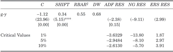
We first look at the long run before turning to issues of cyclicality. The long-run relationship between government expenditure and GDP is explored using least squares regression with Newey-West heteroscedasticity and autocorrelation consistent standard errors. In Table 1, we present the results of a regression of the difference of real government expenditure and real output (g-y) on the irresponsibility dummy, thus making the theoretically attractive imposition of a unitary long-run coefficient in the regression of real government expenditure on real output. The irresponsibility dummy is

Table 1: Long-Run Difference Relationship with Irresponsibility Dummy

C SHIFT RBAR2 _{DW ADF RES NG RES ERS RES}

g-y –1.12 0.34 0.55 0.68

(23.96) (5.15)*** (–2.38) (–9.11) (2.99)

[0.00] [0.00] [0.15]

Critical Values 1% –3.6329 –13.80 1.87

5% –2.9484 –8.10 2.97

10% –2.6130 –5.70 3.91

Notes: t values in parentheses; p-values in square brackets. Independent variable g-y is the difference between the logs of real government spending and real GDP. SHIFT is a dummy variable which captures periods of fiscal irresponsibility and takes a value of 1 from 1977 to 1986 inclusive. ADF refers to the Augmented Dickey-Fuller test, NG to the Ng-Perron Modified Unit Root Test, and ERS to the Elliott-Rothenberg Point Optimal Unit Root Test.

Table 2: Short-Run Cyclicality – Unit Root Tests

Augmented

Dickey-Fuller Test DY DG DAUTOCT DTRANFD DCONFD DINVFD

(–2.540) (–5.661) (–3.775) (–2.929) (–5.737) (–3.658)

[0.1152] [0.0000] [0.0072] [0.0561] [0.0000] [0.0095]

Critical Values 1% –3.639 –3.639 –3.646 –3.724 –3.646 –3.639

5% –2.951 –2.951 –2.954 –2.968 –2.954 –2.951

10% –2.614 –2.614 –2.616 –2.617 –2.616 –2.614

Notes:t values in parentheses; p-values in square brackets. DY is the real GDP growth rate; DG is the percentage change in real government expenditure; DINVFD is the percentage change in real feasible discretionary government investment; DCONFD is the percentage change in real feasible discretionary government consumption; DTRANFD is the percentage change in real feasible discretionary current transfers; DAUTOCT is the percentage change in residual discretionary consumption and transfers.

Sources: Central Statistics Office, Department of Finance.

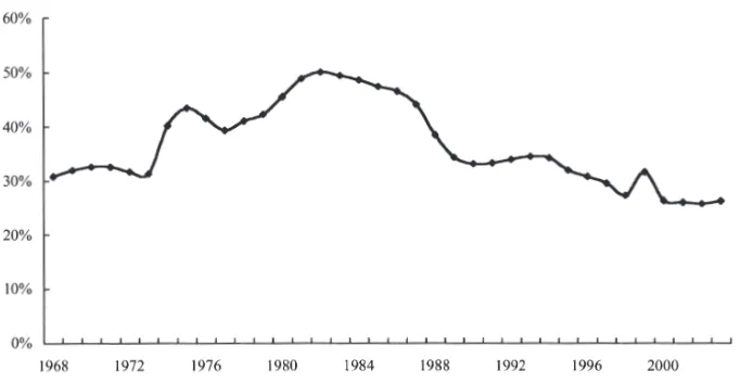
Figure 1: Government Share of GDP

Note: Figure 1 shows Total Government Spending expressed as a percentage of Gross Domestic Product on an annual basis

in the residuals. Additional testing is warranted give the low power of the ADF test and the superior power and size properties of the Ng-Perron and

Elliott-Rothenberg tests.2_{It is intuitively consistent to argue that there must be some}

long-term, non-spurious relationship between government expenditure and output and on foot of our cointegration findings, we include an error-correcting mechanism in our evaluation of the short term.

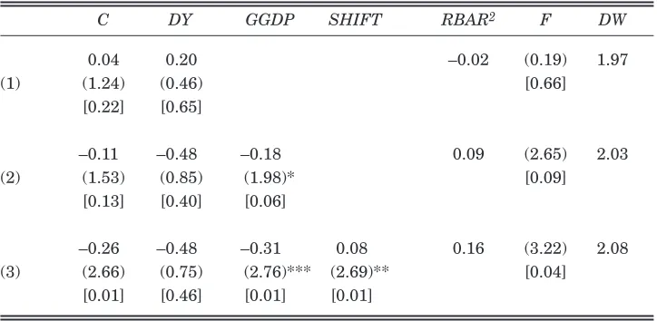
Turning to the short run, we examined the relationship between the various measures of government expenditure outlined above and a number of independent variables using least squares regression with Newey-West heteroscedasticity and autocorrelation consistent standard errors. In Table 3, we present the results of our first set of short-run regressions with total government spending taking the role of the dependent variable.

Our results suggest that the rate of economic growth has little impact on overall government spending growth as the estimated coefficient of DY is insignificantly different from zero in each of the regressions. This allows us to reject the hypothesis of cyclicality in Irish government expenditure. However, the inclusion of a variable which captures the relationship between

Table 3:Short-Run Cyclicality – Total Government Spending

C DY GGDP SHIFT RBAR2 _{F DW}

0.04 0.20 –0.02 (0.19) 1.97

(1) (1.24) (0.46) [0.66]

[0.22] [0.65]

–0.11 –0.48 –0.18 0.09 (2.65) 2.03

(2) (1.53) (0.85) (1.98)* [0.09]

[0.13] [0.40] [0.06]

–0.26 –0.48 –0.31 0.08 0.16 (3.22) 2.08

(3) (2.66) (0.75) (2.76)*** (2.69)** [0.04]

[0.01] [0.46] [0.01] [0.01]

Notes: t values in parentheses; p-values in square brackets. Independent variables: GGDP is the difference between the log of real government expenditure and real GDP lagged by one year; SHIFT is a dummy variable which captures periods of fiscal irresponsibility and takes a value of 1 from 1977 to 1986 inclusive. Dependent variable: DG is the percentage change in real government expenditure. ***, **, * denote significance at the 1, 5 and 10 per cent levels respectively.

Sources:Central Statistics Office, Department of Finance

government expenditure and GDP (GGDP) as an independent variable has a positive impact on the regression’s explanatory power. In each case, the estimated coefficient of GGDP is significantly different from zero with the null

of δ= 0 being rejected at a p-value of 0.01 when a dummy variable designed to

capture the impact of a period of fiscal policy irresponsibility (SHIFT) is included. The GGDP variable is negatively signed. This result is intuitively appealing as it suggests that the greater the size of government, the less willing policymakers are to engage in further spending expansionism. The regression results in Table 3 clearly indicate that the desire to shrink the size of government spending or the imperative of fiscal parsimony has a far more significant role to play in explaining momentum in total government spending than the vagaries of the economic cycle.

The introduction of the SHIFT dummy variable should be significant. A priori, we would expect government spending growth to be higher in the years 1977 to 1986 given the deterioration in the quality of fiscal management which occurred in that period. As expected, the SHIFT variable has a marked and positive impact on the regression’s explanatory power and it is statistically significant at the 5 per cent level. Following logic, the SHIFT dummy is

positively signed.3

3_{Where lagged dependent variables are used throughout this paper, we eschew reporting a} Durbin-Watson d test statistic as that test assumes that the regression model does not include lagged values of the dependent variable. In its stead, the Breusch-Godfrey Lagrange Multiplier test is used. The null hypothesis of this test is that there is no serial correlation in the residuals.

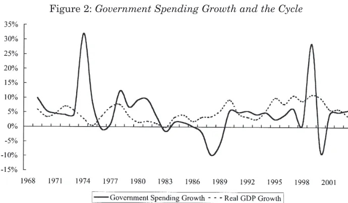
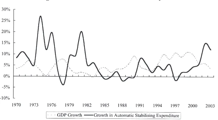
Figure 2: Government Spending Growth and the Cycle

Overall, the evidence in Table 3 suggests that total government expenditure growth is acyclical with the imperative of fiscal parsimony, as measured by the GGDP variable, having a significant influence on spending momentum. Moreover, overall spending growth tends to be higher during periods of policy irresponsibility.

However, the results generated for overall government expenditure may well be camouflaging conflicting cyclical momentum among its component parts. Each of these components is examined in turn. It is reasonable to assume that automatic stabilisers will be the component of public expenditure which is most markedly counter-cyclical. The evidence of our analysis is strongly supportive of this contention as presented in Table 4. The GDP growth rate (DY) is statistically significant in each of the regressions presented in the table and, in all but the simplest model, is significant at the 1 per cent level. Moreover, the coefficient is negatively signed throughout pointing to strong counter-cyclicality in the automatic stabilising component of government expenditure. The simplest model with DY as the sole independent variable reports a low DW d statistic (1.38) that highlights the risk of excluded variable specification bias. The inclusion of the fiscal parsimony imperative (GGDP) as an independent variable augments the

explanatory power of the regression with the adjusted R2_{increasing to 0.31.}

The GGDP variable is strongly significant at the 1 per cent level in two of the regressions reported and is negatively signed in each regression suggesting that larger government output shares serve to restrain the efficacy of automatic stabilisers.

The addition of the SHIFT dummy does not augment the explanatory power of the regression and the variable is statistically insignificant. This result is intuitive as it suggests that bouts of budgetary irresponsibility have little impact on the automatically stabilising elements of government spending. Overall, the evidence of this set of regressions is strongly supportive of the view that automatic stabilisers are efficiently counter-cyclical in an Irish context with the level of economic growth being the prime determinant of growth in this expenditure component. The size of government is of secondary importance in this expenditure category.

T

able 4:

Short-Run Cyclicality – Automatic Stabilisers

CD Y GGDP LDV SHIFT RBAR 2 FD W BG-LM 0.1 1 –0.86 0.12 (5.50) 1.38 (1) (3.45) (2.41)** [0.026] [0.002] [0.020] –0.05 –1.57 –0.19 0.31 (8.55) 1.86 (2) (0.94) (4.23)*** (3.27)*** [0.001] [0.352] [0.000] [0.003] –0.06 –1.42 –0.19 0.19 0.33 (6.17) 0.20 (3) (1.33) (3.17)*** (3.20)*** (1.77)* [0.002] [0.19] [0.004] [0.003] [0.08] –0.06 –1.42 –0.18 0.19 –0.01 0.30 (4.47) 0.21 (4) (0.69) (3.13)*** (2.34)** (1.74)* (0.07) [0.006] [0.50] [0.004] [0.03] [0.09] [0.95] Notes:

t values in parentheses; p-values in square brackets. BG-LM is the p-value from the Breusch-Godfrey Lagrange Multiplier test fo

r first

order serial correlation in the residuals. Independent variables: GGDP

is the difference between the log of real government expe

nditure and

real GDP

lagged by one year; DY is the real GDP

growth rate; LDV is the value of the dependent variable lagged by one year

. SHIFT

is a dummy

variable which captures periods of fiscal irresponsibility and takes a value of 1 from 1977 to 1986 inclusive. Dependent variab

le: DG is the

percentage change in real residual discretionary consumption and transfers. ***, **, * denote significance at the 1, 5 and 10 p

er cent levels

respectively

.

Sources:

Central Statistics Office, Department of Finance; Department of Social and Family

Affairs; The Economic and Social

Research

T

able 5:

Short-Run Cyclicality – Feasible Discretionary Consumption

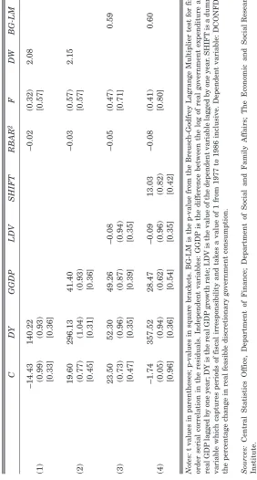
CD Y GGDP LDV SHIFT RBAR 2 FD W BG-LM –14.43 140.22 –0.02 (0.32) 2.08 (1) (0.99) (0.93) [0.57] [0.33] [0.36] 19.60 296.13 41.40 –0.03 (0.57) 2.15 (2) (0.77) (1.04) (0.93) [0.57] [0.45] [0.31] [0.36] 23.50 52.30 49.26 –0.08 –0.05 (0.47) 0.59 (3) (0.73) (0.96) (0.87) (0.94) [0.71] [0.47] [0.35] [0.39] [0.35] –1.74 357.52 28.47 –0.09 13.03 –0.08 (0.41) 0.60 (4) (0.05) (0.94) (0.62) (0.96) (0.82) [0.80] [0.96] [0.36] [0.54] [0.35] [0.42] Notes:

t values in parentheses; p-values in square brackets. BG-LM is the p-value from the Breusch-Godfrey Lagrange Multiplier test fo

r first

order serial correlation in the residuals. Independent variables: GGDP

is the difference between the log of real government expe

nditure and

real GDP

lagged by one year; DY is the real GDP

growth rate; LDV is the value of the dependent variable lagged by one year

. SHIFT

is a dummy

variable which captures periods of fiscal irresponsibility and takes a value of 1 from 1977 to 1986 inclusive. Dependent variab

le: DCONFD is

the percentage change in real feasible discretionary government consumption. Sources:

Central Statistics Office, Department of Finance; Department of Social and Family

Affairs; The Economic and Social

Research

T

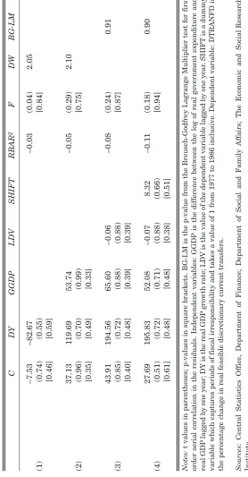
able 6:

Short-Run Cyclicality – Feasible Discretionary Current T

ransfers CD Y GGDP LDV SHIFT RBAR 2 FD W BG-LM –7.53 –82.67 –0.03 (0.04) 2.05 (1) (0.74) (0.55) [0.84] [0.46] [0.59] 37.13 1 19.69 53.74 –0.05 (0.29) 2.10 (2) (0.96) (0.70) (0.99) [0.75] [0.35] [0.49] [0.33] 43.91 194.56 65.60 –0.06 –0.08 (0.24) 0.91 (3) (0.85) (0.72) (0.88) (0.88) [0.87] [0.40] [0.48] [0.39] [0.39] 27.69 195.83 52.08 –0.07 8.32 –0.1 1 (0.18) 0.90 (4) (0.51) (0.72) (0.71) (0.88) (0.66) [0.94] [0.61] [0.48] [0.48] [0.38] [0.51] Notes:

t values in parentheses; p-values in square brackets. BG-LM is the p-value from the Breusch-Godfrey Lagrange Multiplier test fo

r first

order serial correlation in the residuals. Independent variables: GGDP

is the difference between the log of real government expe

nditure and

real GDP

lagged by one year; DY is the real GDP

growth rate; LDV is the value of the dependent variable lagged by one year

. SHIFT

is a dummy

variable which captures periods of fiscal irresponsibility and takes a value of 1 from 1977 to 1986 inclusive. Dependent variab

le: DTRANFD is

the percentage change in real feasible discretionary current transfers. Sources:

Central Statistics Office, Department of Finance; Department of Social and Family

Affairs; The Economic and Social

Research

parsimony imperative (GGDP), momentum indicators (LDV) and the irresponsibility dummy have extremely poor explanatory power. In fact, in no instance in these sets of regressions can we reject the null hypothesis that the true coefficient is zero. Our analysis suggests that real growth in feasible discretionary consumption and feasible discretionary current transfers is

orthogonal to economic fundamentals.4

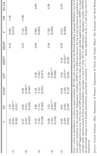
The results for feasible discretionary government investment are presented in Table 7. As discussed earlier, this should be the component of government expenditure that demonstrates the least amount of cyclicality due to its multi-year nature in terms of both planning and delivery.

The results of the two simplest regressions with DY alone and DY and GGDP used as regressors provide conflicting signals in terms of the statistical significance of the independent variables. Moreover, DW statistics which lie below and within (respectively) the zone of indecision at the 5 per cent significance level alert us to the possible presence of positive autocorrelation

4_{We tested for the impact of different definitions of discretion by running a set of regressions} where all changes in both public sector pay and welfare payments rather than those payments in excess of inflation are treated as discretionary. The results show that adjusted current transfers are negatively correlated with the output growth rate and the government share of GDP at the 1 per cent level. Adjusted consumption is negatively correlated with the relationship between government spending and output at the 1 per cent level. These regressions point to the presence of a cyclical element in inflation and also suggest that spending growth in these expenditure categories above an inflation-proofing level is not influenced by economic considerations.

Figure 3:Automatic Stabilisers and the Cycle

in the error terms. We suspect that we are dealing with a case of excluded variable specification bias. With the inclusion of a lagged dependent variable, the null hypothesis of no serial correlation is not rejected using the results of the Breusch-Godfrey Lagrange Multiplier test. Moreover, the lagged dependent variable is significant at the 10 per cent level when it is included with the DY and GGDP variables. However, its inclusion impacts negatively on the significance of the GGDP variable and we can no longer reject the null hypothesis that the true value of the GGDP coefficient is equal to zero. This result encourages us to risk specification bias by dropping the GGDP variable from the regression.

This move leaves us with two strongly significant independent variables in the form of DY and LDV with the null that the true value of the coefficients are zero being rejected at a p-value of 0.002 and 0.000 respectively. The evidence suggests that feasible discretionary government investment is impacted by a different set of influences than overall government expenditure. The results of the limited regression suggest that feasible discretionary government investment is strongly pro-cyclical and carries momentum from the previous year. The latter result is understandable given the multi-year nature of government capital formation planning.

Most interest, however, centres on the cyclicality result. Given the relative size of the estimated coefficients (1.53 in the case of real GDP growth and 0.39 in the case of the lagged dependent variable), our results suggest that current economic activity is a considerably more potent influence on the resources

Figure 4: Feasible Discretionary Investment and the Cycle

T

able 7:

Short-Run Cyclicality – Feasible Discretionary Investment

CD Y GGDP LDV SHIFT RBAR 2 FD W BG-LM –0.04 1.70 0.15 (6.90) 1.36 (1) (0.94) (2.63)** [0.013] [0.36] [0.01] –0.27 0.65 –0.28 0.27 (7.14) (7.06) (2) (2.43) (0.81) (2.06)** [0.003] [0.021] [0.423] [0.047] –0.18 0.96 –0.16 0.29 0.30 (5.69) 0.60 (3) (1.45) (1.14) (1.10) (1.83)* [0.003] [0.156] [0.263] [0.351] [0.077] –0.06 1.53 0.39 0.28 (7.52) 0.59 (4) (1.55) (3.45)*** (3.90)*** [0.002] [0.132] [0.002] [0.000] (5) –0.40 0.91 –0.34 0.24 0.10 0.35 (5.51) 0.55 (2.30) (0.94) (1.62) (2.07)** (2.52)** [0.002] [0.03] [0.36] [0.12] [0.05] [0.02] Notes:

t values in parentheses; p-values in square brackets. BG-LM is the p-value from the Breusch-Godfrey Lagrange Multiplier test fo

r first

order serial correlation in the residuals. Independent variables: GGDP

is the difference between the log of real government expe

nditure and

real GDP

lagged by one year; DY is the real GDP

growth rate; LDV is the value of the dependent variable lagged by one year; SHIFT

is a dummy

variable which captures periods of fiscal irresponsibility and takes a value of 1 from 1977 to 1986 inclusive. Dependent variab

le: DINVFD is

the percentage change in real feasible discretionary government investment. ***, **, * denote significance at the 1, 5 and 10 p

er cent levels

respectively

.

Sources:

Central Statistics Office, Department of Finance; Department of Social and Family

Affairs; The Economic and Social

Research

made available for feasible discretionary investment than multi-year budgeting. As such, the results can be interpreted as indicating a short-termist approach on the part of domestic policymakers to government-funded fixed capital formation.

V THE IMPACT OF FORECASTS

Given the evidence of pro-cyclicality in feasible discretionary government investment reported earlier, we conducted a series of regressions to test the relative importance of actual and forecast growth rates in determining this component of public expenditure. The results are presented in Tables 8 and 9.

In Table 8, the actual growth rate is excluded as an independent variable while the forecast growth rate, given by the mean of the Department of Finance’s and the OECD’s published forecast growth rates, is included. This is a reasonable approach to take as forward spending decisions, as presented in the annual Budget, are based on growth projections rather than actual outturns. The results presented in Table 8 report that the forecast growth rate is statistically insignificant as an explanatory variable where overall government spending, feasible discretionary consumption expenditure and feasible discretionary current transfers are the dependent variables. This suggests that growth forecasts have little bearing on budget decisions in

Figure 5: GDP Growth Rates

T

able 8:

Impact of Forecasts on Spending Decisions

C GGDP LDV DYMEAN SHIFT RBAR 2 BG-LM DG –0.29 –0.34 0.04 –0.74 0.09 0.12 0.45 (1) (2.28) (2.24)** (0.19) (0.88) (2.59)** [0.03] [0.03] [0.85] [0.38] [0.02] DAUTOCT –0.13 –0.23 0.22 –1.77 0.03 0.16 0.60 (2) (1.53) (3.15)*** (1.68) (2.87)*** (0.79) [0.14] [0.004] [0.1 1] [0.01] [0.44] DCONFD 0.32 66.10 –0.09 706.97 –1.1 1 –0.07 0.42 (3) (0.55) (0.78) (1.01) (0.96) (0.09) [0.58] [0.45] [0.32] [0.35] [0.93] DINVFD –0.28 –0.19 0.13 2 .80 0 .05 0.43 0.96 (4) (1.62) (0.97) (1.89)* (2.50)** (1.05) [0.12] [0.34] [0.07] [0.02] [0.30] DTRANFD 14.23 26.07 –0.05 –79.60 9.73 –0.12 0.86 (5) (0.35) (0.54) (0.90) (0.21) (0.65) [0.73] [0.59] [0.37] [0.84] [0.52] Notes:

t values in parentheses; p-values in square brackets. Independent variables; GGDP

is the difference between the log of real gove

rnment

expenditure and real GDP

lagged by one year; LDV is the value of the dependent variable lagged by one year; DYMEAN is the averag

e of the

forecast growth rates of the Department of Finance and the OECD; and SHIFT is a dummy variable which captures periods of fiscal irresponsibility and takes a value of 1 from 1977 to 1986 inclusive. Dependent variables: DG is the percentage change in real g

overnment

expenditure; DAUTOCT is the percentage change in real residual discretionary consumption and transfers; DCONFD is the percentag

e change

in real feasible discretionary government consumption; DINVFD is the percentage change in real feasible discretionary governmen

t investment;

and DTRANFD is the percentage change in real feasible discretionary current transfers. ***,** ,* denote significance at the 1,

5 and 10 per cent

levels respectively

.

Sources:

relation to overall expenditure, transfer payments or feasible discretionary consumption.

However, the forecast growth rate is statistically significant at the 1 per cent level where real growth in automatic-stabilising expenditure is the dependent variable. When the actual growth rate is added as an explanatory variable, as shown in Table 9, the forecast growth rate is no longer statistically significant while the actual growth outturn is significant at the 1 per cent level. With the coefficient being negatively signed, this result is intuitively appealing: automatic stabilising expenditure growth should have an inverse relationship with economic growth and should be more potently affected by actual rather than forecast activity levels. The fiscal parsimony variable is also significant at the 1 per cent level where the actual growth rate is excluded and at the 5 per cent level where it is included as an independent variable. It is negatively signed suggesting that the efficacy of automatically stabilising expenditure is adversely impacted by excessive government expenditure.

In the regression where feasible discretionary government investment is the dependent variable, the mean growth forecast and the lagged dependent variable are the only statistically significant independent variables. Moreover, the null hypothesis that the true value of the forecast coefficient equals zero is

rejected at a p-value of 0.02. The adjusted R2 _{in the case of this regression}

where feasible discretionary investment growth is the dependent variable in Table 8 is the highest encountered in the analysis conducted for this paper at 0.43. This result is intuitively appealing as it is most sensible for policymakers to plan investment spending levels on the basis of growth forecasts. When we

add the actual growth rate as an explanatory variable, the adjusted R2 _eases

slightly to 0.41 while the mean forecast growth rate becomes the only statistically significant explanatory variable. We reject the null hypothesis that the true value of the forecast coefficient equals zero at a p-value of 0.01. The strength of the relationship between actual feasible discretionary

investment growth and forecast GDP growth levels suggests that

policymakers have great faith in their own forecasts. The size of the coefficient of forecast growth, at 3.23 where the actual growth outturn is included as an independent variable, suggests, once again, that feasible discretionary investment spending is strongly pro-cyclical. The significance of the various forecasts combined with the size of the coefficients suggests that this sub-component of government expenditure is deliberately pro-cyclical.

T

able 9:

Impact of Forecasts on Spending Decisions (Control with Actual Growth Rates) C

GGDP DY LDV DYMEAN SHIFT RBAR 2 BG-LM DG –0.28 –0.33 –0.36 0.01 –0.33 0.08 0.10 0.31 (1) (1.96) (2.1 1)** (0.39) (0.07) (0.26) (1.77)* [0.06] [0.04] [0.70] [0.94] [0.80] [0.09] DAUTOCT –0.08 –0.21 –1.29 0.17 –0.42 0.01 0.28 0.42 (2) (1.01) (2.65)** (2.87)*** (1.38) (0.82) (0.19) [0.32] [0.01] [0.01] [0.18] [0.42] [0.85] DCONFD 25.95 62.79 175.56 –0.10 515.51 2.89 –0.10 0.43 (3) (0.46) (0.75) (0.79) (0.97) (0.95) (0.20) [0.65] [0.46] [0.44] [0.34] [0.35] [0.84] DINVFD –0.27 –0.19 –0.35 0.10 3.23 0.04 0.41 0.86 (4) (1.58) (0.95) (0.33) (0.85) (2.88)*** (0.84) [0.13] [0.35] [0.75] [0.41] [0.01] [0.41] DTRANFD 1.54 20.19 379.14 –0.07 494.63 18.18 –0.15 0.25 (5) (0.04) (0.40) (0.83) (0.88) (0.68) (0.84) [0.97] [0.69] [0.41] [0.39] [0.50] [0.41] Notes:

t values in parentheses; p-values in square brackets. Independent variables; GGDP

is the difference between the log of real gove

rnment

expenditure and real GDP

lagged by one year; LDV is the value of the dependent variable lagged by one year; DY is the actual rea

l GDP

growth

rate; DYMEAN is the average of the forecast growth rates of the Department of Finance and the OECD; and SHIFT is a dummy variab

le which

captures periods of fiscal irresponsibility and takes a value of 1 from 1977 to 1986 inclusive. Dependent variables: DG is the

percentage change

in real government expenditure; DAUTOCT is the percentage change in real residual discretionary consumption and transfers; DCON

FD is the

percentage change in real feasible discretionary government consumption; DINVFD is the percentage change in real feasible discr

etionary

government investment; and DTRANFD is the percentage change in real feasible discretionary current transfers. ***,** ,* denote

significance

at the 1, 5 and 10 percent levels respectively

.

Sources:

Table 10: Short-Run Cyclicality – IV Estimation

C DY GGDP SHIFT LDV RBAR2 _F

GOV –0.26 –0.48 –0.31 0.08 0.16 (3.22)

(1) (2.66) (0.75) (2.76)*** (2.69)** [0.04]

OLS [0.01] [0.46] [0.01] [0.01]

GOV –0.29 –1.33 –0.38 0.08 0.08 (2.92)

(2) (2.52) (1.13) (2.69)** (1.87)* [0.05]

TSLS [0.02] [0.27] [0.01] [0.07]

AUTO –0.06 –1.42 –0.18 –0.01 0.19 0.30 (4.47)

(3) (0.69) (3.13)*** (2.34)** (0.07) (1.74)* [0.006]

OLS [0.50] [0.004] [0.03] [0.95] [0.09]

AUTO –0.08 –2.09 –0.24 –0.002 0.10 0.24 (2.34)

(4) (0.85) (1.59) (1.76)* (0.06) (0.43) [0.08]

TSLS [0.40] [0.12] [0.09] [0.95] [0.67]

CON –1.74 357.52 28.47 13.03 –0.09 –0.08 (0.41)

(5) (0.05) (0.94) (0.62) (0.82) (0.96) [0.80]

OLS [0.96] [0.36] [0.54] [0.42] [0.35]

CON 3.84 514.50 42.21 13.38 –0.11 –0.09 (0.23)

(6) (0.06) (0.68) (0.48) (0.54) (0.53) [0.92]

TSLS [0.96] [0.51] [0.63] [0.59] [0.60]

TRAN 27.69 195.83 52.08 8.32 –0.07 –0.11 (0.18)

(7) (0.51) (0.72) (0.71) (0.66) (0.88) [0.94]

OLS [0.61] [0.48] [0.48] [0.51] [0.38]

TRAN 9.24 –253.43 10.45 7.95 –0.02 –0.14 (0.16)

(8) (0.08) (0.21) (0.07) (0.20) (0.10) [0.96]

TSLS [0.94] [0.84] [0.94] [0.84] [0.92]

INV –0.06 1.53 0.39 0.28 (7.52)

(9) (1.55) (3.45)*** (3.90)*** [0.01]

OLS [0.13] [0.002] [0.000]

INV –0.12 2.80 0.36 0.18 (8.27)

(10) (2.38) (3.03)*** (2.31)** [0.001]

TSLS [0.02] [0.01] [0.03]

VI CONCLUSIONS

The evidence in this paper suggests that while Irish government expenditure is in aggregate acyclical, there are substantial differences in the cyclicality of the sub-components. Overall government expenditure appears to be more strongly influenced by considerations of fiscal probity rather than the rate of GDP growth. However, our analysis of disaggregated expenditures suggests that this overall result serves to camouflage the co-existence of marked pro- and counter-cyclicality. Automatic stabilisers report a pronounced counter-cyclicality which is appealing from an efficiency viewpoint and underpinned by theoretical considerations. Two of the new sub-components of expenditure which we examined, namely feasible discretionary government consumption and feasible discretionary current transfers show no evidence of any cyclicality. In fact, there seems to be no relation between these series and any of the independent variables we identified for this paper. We conclude that momentum in these areas where policymakers have real discretion and full freedom to manoeuvre is orthogonal to economic fundamentals.

Our analysis points to marked pro-cyclicality in feasible discretionary government investment. Moreover, official growth forecasts are more statistically significant in the relevant regressions than actual growth outturns. This finding leads us to the conclusion that, not only is government feasible discretionary investment pro-cyclical, it is deliberately so. The Department of Finance does appear to have believed prevailing consensus forecasts over the period under study. The evidence we present strongly supports the contention that when Irish policymakers have the money, they spend it on feasible discretionary investment. As a consequence, we can conclude that government investment has been the residual in the Irish budgetary process over the 1969 to 2003 period.

This approach to the allocation of capital resources imposes clear short-term restraints on the effective management of the economic cycle and could, through a stop-start approach to government-funded capital formation, reduce the economy’s sustainable growth potential. The hope must be that recent changes to the capital resource allocation structure, outlined below, will reduce the pronounced pro-cyclicality of feasible discretionary investment.

capital subhead. The commitment to allocate 5 per cent of (forecast) GNP should significantly reduce the cyclicality of government investment over the years ahead.

REFERENCES

BACKUS, D. K., P. J. KEHOE, and F. E. KYDLAND, 1995. “International

Business Cycles: Theory and Evidence”, Frontiers of Business Cycle

Research, Princeton University Press, pp. 331-356.

BARRO, R. J., 1979. “On the Determination of the Public Debt”, Journal of

Political Economy,Vol. 87, pp. 940-971.

BARRO, R. J., 1989. “The Ricardian Approach to Budget Deficits”, Journal of

Economic Perspectives, Vol. 3, No. 2, pp. 37-54.

BARRO, R. J., 1990. “Government Spending in a Simple Model of Endogenous

Growth”, Journal of Political Economy,Vol. 98, No. 5, pp. 103-126.

BLANCHARD, O. and S. FISCHER, 1989. “Lectures on Macroeconomics”, The

MIT Press, Cambridge MA.

EICHENBAUM, M., 1997. “Some Thoughts on Practical Stabilization Policy”,

American Economic Review, Vol. 87, No. 2, pp. 236-239.

ELLIOTT, G., T. ROTHENBERG and J. STOCK, 1996. “Efficient Test for an

Autoregressive Unit Root”, Econometrica, Vol. 64, pp 813-836.

ENGLE, R. F. and C. W. J. GRANGER, 1987. “Cointegration and Error

Correction: Representation, Estimation and Testing”, Econometrica, Vol.

55, No. 2, pp. 251-276.

GALI, J., and R. PEROTTI, 2003. “Fiscal Policy and Monetary Integration in

Europe”, Economic Policy, Vol. 18, No. 37, pp. 533-572.

GAVIN, M., and R. PEROTTI, 1997. “Fiscal policy in Latin America”, NBER

Macroeconomics Annual 1997, Vol. 12, pp. 11-61.

LANE, P. R., 1998. “On the Cyclicality of Irish Fiscal Policy”, The Economic

and Social Review, Vol. 29, No. 1, pp. 1-16.

LANE, P. R., 2003. “The Cyclical Behaviour of Fiscal Policy: Evidence from the

OECD”, Journal of Public Economics, Vol. 87, No.12, pp. 2661-2675.

NG, S. and P. PERRON, 2001. “Lag Length Selection and the Construction of

Unit Root Tests with Good Size and Power”, Econometrica, Vol. 69, pp

1519-1554.

SORENSEN, B. E., L. WU and O. YOSHA, 2001. “Output Fluctuations and

Fiscal Policy: US State and Local Governments 1978-1994”, European

Economic Review, Vol. 45, pp. 1271-1310.

TALVI, E. and C. VEGH, 2000. “Tax Base Variability and Pro-cyclical Fiscal

TAYLOR, J., 2000. “Reassessing Discretionary Fiscal Policy”, Journal of

Economic Perspectives, Vol. 14, pp. 21-36.

TORNELL, A. and P. R. LANE, 1999. “The Voracity Effect”, American

APPENDIX I: DATA SOURCES & ISSUES

Social security data were drawn from the annual Statistical Abstract of

Ireland and from the annual Statistical Report of the Department of Social

and Family Affairs.

National accounts data were taken from the CSO’s annual National

Income & Expenditure publications.

Fiscal data were drawn from the Department of Finance’s annual Finance

Accounts.

Numbers employed in the public sector were sourced from the Labour

Force Surveyand provided by the Economic and Social Research Institute.

Growth forecasts are taken from the OECD’s June Economic Outlookand

individual country report publications and the Department of Finance’s

Economic Reviewand Outlookpublications.

Live register data were provided by Datastream.

Fiscal years:Until 1974, Irish fiscal accounts were prepared on the basis

of the old fiscal year, April 6th to April 5th. 1975 was the first year in which calendar-based data were made available. Adjustments are made to previous years’ data using spending growth trends to produce calendar estimates for the period 1969 to 1974.

Euro changeover:In 1999, Ireland joined Economic and Monetary Union

and from 2001 all data releases are denominated solely in euro. The necessary adjustment for comparability is made by converting euro amounts into punts at the irrevocable fixed rate at which Ireland joined the single currency.

Establishment of An Post and Telecom Éireann: These entities were

previously part of central government and their expenditures were treated as government consumption and investment until 1984. Amounts spent by the predecessor of these bodies were excluded for the period 1969 to 1984 for comparability purposes.

No explicit discretionary/non-discretionary capital split for 1969-1973:To

overcome this data deficiency we assume that the average discretionary/non-discretionary capital expenditure split for the period 1969-1973 was the same as that in the 1975-1977 period.

Number of Social Welfare Beneficiaries:This data series is incomplete. A

APPENDIX II: UNIT ROOT TESTS

The results of our unit root tests are presented in Table 2. For all the variables presented here other than real GDP growth (DY) and real feasible discretionary current transfers growth (DTRANFD), we can confidently reject the null hypothesis that there is a unit root and each of these time series is stationary. In the cases of real government expenditure growth (DG), growth in automatic stabiliser expenditure (DAUTOCT) and real feasible discretionary government consumption growth (DCONFD), the null hypothesis can be rejected at the 1 per cent level. In the case of real feasible discretionary investment growth (DINVFD), the null hypothesis of a unit root can be rejected at the 5 per cent level while the null can be rejected at the 10 per cent level in the case of real feasible discretionary current transfers growth (DTRANFD). In relation to real GDP growth, the test results suggest that this time series is borderline non-stationary with a p-value of 0.115. However, it is reasonable to treat DY as a stationary variable given theoretical support: GDP growth rates do have a mean-reverting tendency.

APPENDIX III: INSTRUMENTAL VARIABLE ESTIMATION