Return on sales and wheat yields per hectare of European agricultural entities

Agriculture is an important part of the national economy. It produces food and other products and has an impact on manufacturing industries. From this point of view, it is a very important industry, although its share in GDP is very low in comparison with other industries. Based on the national accounts statistics, the agricultural sector in the Czech Republic shared in the total gross value added of the Czech Republic and similarly the EU by 1.68 and 1.7%, respectively (Institute of Agricultural Economics of the Czech Republic 2016; Eurostat 2016).

The structure and size of agricultural entities in the EU are highly varied. Family farms dominate in some states (Poland, Slovenia), while transformed cooperatives prevail in others (Slovakia, the Czech Republic), or there is a combination of both (Hungary, Romania) (Záhorský and Pokrivčák 2017).

Agricultural production has a biological character, it depends on natural conditions, and as a result, the production process is relatively less controllable by humans. The use of modern technologies does not produce results comparable to other sectors.

The performance of agricultural entities is typically monitored at the level of macroeconomic indicators,

combined with the quantity of agricultural produc-tion units (Sarris et al. 1999; Bijman et al. 2012; Golas 2016; Jedruchniewicz and Danilowska 2016; Věžník et al. 2017).

Another way to measure performance is profitability, i.e. the ability to gain profit based on funds invested. Empirical research most commonly uses the indicators of return, return on equity (ROE), return on assets (ROA), return on sales (ROS) presented in studies of Mishra et al. (2009); Circiumaru et al. (2010). These indicators are most commonly used in the industrial sector (Cucchiella 2015; Brierley 2016). Empirical studies on the evaluation of profitability based on the indicators of financial analysis are not very frequent in agriculture. The performance of agricultural enti-ties measured by profit and value added was pub-lished by Miklovičová and Gurčík (2009) and Vuckovic et al. (2016); the development of profit and profitability were explored by Chrastinová (2008) and Svoboda and Novotná (2011). All the authors confirm a relationship between the indicators of profitability and the specific conditions of agricultural production. At the same time, they point out the impact of subsidies on these indicators. Szymanska (2015) examined the impact

Return on sales and wheat yields per hectare

of European agricultural entities

Eva HYBLOVA*, Roman SKALICKY

Faculty of Economics and Administration, Masaryk University, Brno, Czech Republic

*Corresponding author: hyblova@econ.muni.cz

Hyblova E., Skalicky R. (2018): Return on sales and wheat yields per hectare of European agricultural entities. Agric. Econ. – Czech, 64: 436–444.

Abstract: Performance of agricultural entities can be observed from several different perspectives: using macroecono-mic indicators, the quantity of agricultural production units, or by measuring the profitability. The paper present focuses on the relationship between profitability, return on sales (ROS) and wheat yields per hectare in agricultural entities in member states of the European Union (EU), divided into size categories by quantity standard output (SO). Due to the high proportion of subsidies in agriculture, the ROS indicator was rated in two versions: including subsidies and excluding subsidies. The aim of the paper is to confirm or refute the mutual relationship between these indicators, i.e. wheat yields per hectare, return on sales, and the size of the farm.The comparison is performed by means of indicators of descriptive statistics and tests of mathematical statistics. The results of the research show that return on sales drops with the size of the farm, while yields per hectare grow.

Keywords: agricultural entities, agricultural production, performance, profitability, return on sales

of the selected factors on the return on equity, and she identified the influence of two indicators, return on sales and asset turnover ratio.

The low number of publications on this topic is among other caused by the fact that most of the ex-isting accounting systems do not take into account the specifics of agricultural production and the biological transformation associated with this type of production (Bohušová et al. 2012). According to Sedláček (2010), compared with other economic sectors, agriculture is characterised by specific activities that require an appropriate accounting approach. When that is absent, it is difficult to evaluate and compare the indicators of financial analysis, which use the data from the financial accounting as the input information.

MATERIAL AND METHODS

ROS was selected as an indicator to verify the per-formance. It is a ratio used to evaluate a company’s operational efficiency. ROS is also known as a com-pany’s operating profit margin. ROS is a financial ratio that calculates how efficiently a company is generating profits from its revenues. It measures the performance of a company by analysing the percentage of the total revenue that is converted into the net income.

ROS = (farm net income)/(farm revenue) × 100% (1)

The data analysed come from the Farm Accountancy Data Network database (FADN) (FADN 2016), which is, among other, an instrument for the evaluation of the Common Agricultural Policy (CAP). The member states collect the data annually. It uses a sample of farms that are engaged in agriculture. The goal of sampling is to obtain representative data in the dimensions of the region, economic size, and type of farming; the repeated data collection serves as a basis for the time series of the statistics published by the FADN.

The subject of analysis was data file YEAR A24 ES6 TF8.zip with economic and agricultural statistics in the dimensions year (2004–2013), region (A1) where the farm operates, type of farming (TF8 based on 2003/369 (European Commission (EC)), and eco-nomic size (ES6 based on 2003/369 (EC)). We worked with a file classifying the size of the agricultural farms based on the volume of the standard output (SO), as defined by the Regulation (EC) No. 1242/2008.

SO is the estimated monetary value of the

agri-on the average prices of productiagri-on and agricultural yields per hectare, multiplied by the number of hec-tares available for the farm’s agricultural activities.

It is calculated as follows:

1

SOy =

∑

where SO_y – standard output in year (y); n – num-ber of the main and side products in the year (y); u_yi– amount of units (i) in year (y) (e.g. number of hectares or number of animals); vyi – standardized monetary value of the production unit (i) in year (y). Standardized monetary value is obtained as the mean of the value of a production unit in five years, i.e. for the reference year, two years prior to the reference period, and two years after the reference period, using the following relationship:

2

2 / 5

y

yi y yi

v =

∑

where vyi – standardised monetary value of the production unit (i) in year (y); v_yi–monetary value of the production unit (i) in year (y).

After the size of the farm is expressed in EUR through the SO, the farms are divided into six groups by size (Table 1). The data file further distinguishes eight types of farming (Table 2).

The return on sales of the farms focusing on field crops (fieldcrops) was compared. Because farms in the EU come from different climatic and soil areas, we have only included in the comparison those groups (groups by size and region of activity) that grow wheat. The wheat was chosen as a criterion for the selection as its growing is highly widespread. The presence or absence of its growing in the region thus served as a rough measure of the regional comparability. The FADN database contains the farms in the following coun-tries: Austria, Belgium, Bulgaria, Croatia, Cyprus, the Czech Republic, Denmark, Estonia, Finland, France,

Table 1. Economic size categories of farms in the EU Economic size Standard output value of the farm (EUR)

1 2 000 ≤ 8 000

2 8 000 ≤ 25 000

3 25 000 ≤ 50 000

4 50 000 ≤ 100 000

5 100 000 ≤ 500 000

6 ≥ 500 000

Table 2. Principal type of farming categories

Types of farming (TF8) Principal type of farming

1 fieldcrops

2 horticulture

3 wine

4 other permanent crops

5 milk

6 other grazing livestock

7 granivores

8 mixed

Source: authors‘ calculation based on FADN database (FADN 2016)

Table 3. Average wheat yields of farms in the European Union by economic size based on regions where the wheat was produced in 2004–2013 (100 kg of wheat per ha)

Economic size _{2004 2005 2006 2007 2008}Year_{2009 2010 2011 2012 2013}

1 44.7 33.5 29.7 31.1 38.8 35.3 31.9 39.3 35.5 38.1

2 43.5 41.4 37.4 37.9 44.3 40.2 37.4 40.6 40.5 42.9

3 53.8 51.0 48.6 45.5 54.6 45.3 44.0 46.8 45.7 51.0

4 57.8 55.6 51.3 50.3 56.6 55.3 51.4 51.9 51.3 54.5

5 64.5 58.8 54.0 50.1 59.6 56.2 52.0 52.9 54.2 57.0

6 70.5 68.7 64.0 52.9 70.2 61.7 56.3 57.5 57.6 64.4

Source: authors‘ calculation based on FADN database (FADN 2016)

Germany, Greece, Hungary, Ireland, Italy, Lithuania, Luxembourg, Latvia, Malta, the Netherlands, Poland, Portugal, Romania, Slovakia, Slovenia, Spain, Sweden, the United Kingdom. However, the countries where wheat is not grown or the yields are very low or marginal were not included in the comparison (Cyprus, Greece, Italy, Luxembourg, Malta, Portugal, Slovakia). Some size groups of farms in several countries are not included either (e.g. the smallest farms in the Czech Republic). Additionally, in some countries, some size groups do exist, but they do not grow wheat at all or did not grow it throughout the entire monitoring period (2004–2013, e.g. Ireland). In case of Croatia, the data are available only for the year 2013; in case of Bulgaria and Romania, the data are available for the period 2007–2013 and in case of Slovenia for the period 2006–2013.

Within several countries, the FADN database recognises more production areas (region, A1), for which the indicators are monitored separately.

We decided to average the data of the particular re-gions within a country before the data processing in the countries where the FADN database monitors more regions. Afterwards, we used the data obtained in this way as representatives of the economic indica-tors of agricultural farms in the country. The average wheat yields in the particular countries is presented in Table 3. The average values based on the size cat-egories for the period 2004–2013 are listed in Table 6. We tested the null hypothesis on the equality of the mean values of yields per hectare in the adjoining size categories at 5% level of significance. Except for size categories 4–5, the null hypothesis was rejected.

We explored the relationship between the yields per hectare and return on sales. However, the ag-ricultural sector is under a great effect of subsidies (which is the reason why the FADN database was created). Therefore, we calculated the indicator ROS (Equation 1) in two versions: ROS1 (Equation 4) – in-cluding subsidies and ROS2 (Equation 5) – exin-cluding subsidies. ROS1 was calculated as the share of the farm net income (in EUR) – (SE420) and the total output (in EUR) – (SE131) in percent (Equation 4).

ROS2 was calculated in a similar manner (in percent), just the indicator’s numerator was first adjusted by the balance of the received operating subsidies and taxes (SE600) and the balance of subsidies and taxes related to investment activities (SE405) (Equation 5).

The data for the particular countries by the size of the farm (obtained by averaging over the regions within the country) were further averaged over the EU states based on the farm size for each year ROS1 = (farm net income [SE420])/(total output [SE131]) × 100%

ROS2 = (farm net income [SE420] – balance subsidies & taxes on investments [SE405] – – balance current subsidies & taxes)/(total output [SE131]) × 100%

(4)

of the monitoring period 2004–2013. The values are presented in Tables 4–5.

Statistical methods used for the data process-ing were the statistical description methods. The mathematical statistics methods were used for the statistical hypothesis testing; specifically, the tests for the equality of two variances (F-test) and the test of the equality of two expected values (t-test) were used (Taeger and Kuhnt 2014).

F-test is based on the assumption of normal distri-bution of the observed values. The null hypothesis H₀: 2 2

0

H : σX σY on the equality of variances σ2X and   σY2  is tested against the alternative hypothesis H₁: 2 2

1

H : σ_X σ_Y. 

The test statistic F is defined as a ratio of the vari-ance of a sample of the data:

2

2 X

Y

S F

S

= (6)

where F is F-statistic; 2 X

S is the bigger variance and 2 Y

S

is the smaller variance. X and Y are the two samples of the variables. The variances are defined as follows:

(

)

2

1

1 1

n

X _i i

S X X

n =

= −

−

∑

(

)

2 1 m

S =

∑

where n is the number of units in the sample of vari-able X, X_i is the (ith_{) unit of variable X; Xis the}

aver-age of variables X; m is the number of units in the sample of variable Y, Y_i is the (ith_{) unit of variable Y,}

Y is the average of variables Y.

If F-statistic is greater than the critical value:

(1 – α/2) quintile of F-distribution with n – 1 and m – 1 degrees of freedom, the null hypothesis is rejected.

To test the equality of two populations means, the t-test is used. With the equal sample sizes and equal variance, test statistic t is defined as:

2 / p

X Y t

S n

−

= (9)

where 2 2

2

X Y

p S S

S = + (10)

where t is the t-statistic. The remaining variables are defined the same as in the case of Equations 7–8.

If statistic t is greater than t–distribution with 2n – 2 degrees of freedom for (1 – α/2) quintile, the null hypothesis is rejected.

With the equal or unequal sample sizes and unequal

Table 5. Average returns on sales without subsidies and taxes (ROS2) of farms in the European Union by their econo-mic size based on regions where the wheat was produced in 2004–2013 (% of total output)

Economic size Year

2004 2005 2006 2007 2008 2009 2010 2011 2012 2013

1 20.5 7.4 27.1 24.5 14.9 –11.8 4.1 7.9 11.2 9.2

2 –4.7 –14.2 –12.9 6.5 –5.6 –25.1 –4.4 1.6 4.5 –7.5

3 –4.0 –11.0 –7.7 13.6 –4.2 –25.3 –1.9 6.5 8.3 0.7

4 –1.0 –4.1 –4.8 16.9 –0.8 –19.6 1.3 5.9 11.1 1.2

5 1.9 –3.3 –3.6 11.1 0.4 –15.1 3.6 7.8 13.0 0.9

6 –11.3 –10.3 –11.2 –1.9 –6.4 –24.0 –4.9 2.4 6.4 0.9

Source: authors‘ calculation based on FADN database (FADN 2016)

Table 4. Average returns on sales including subsidies (ROS1) of farms in the European Union by their economic size based on regions where the wheat was produced in 2004–2013 (% of total output)

Economic size Year

2004 2005 2006 2007 2008 2009 2010 2011 2012 2013

1 46.8 37.4 82.1 49.4 49.8 69.0 66.0 68.4 51.9 61.7

2 34.4 35.9 36.8 40.2 36.4 33.9 42.1 43.5 40.8 33.0

3 31.5 27.3 32.9 41.4 34.1 26.2 34.4 39.7 38.5 31.8

4 31.9 30.0 33.6 43.5 31.8 22.0 36.9 35.7 36.7 29.6

5 26.5 21.9 25.3 34.5 25.1 18.3 30.1 29.6 31.6 24.6

6 4.3 5.1 7.7 18.4 12.0 2.7 15.6 20.2 22.9 19.9

2 _/ 2_/

X Y

X Y t

S n S m

− =

+

The degrees of freedom are defined as:

2 2 2

2

2 2

2 . .

1 1

y x

y x

S S

n m

d f

S S

m n

n m

 

+

 

 

 

=

   

 

   

  ₊ 

− −

(12)

RESULTS AND DISCUSSION

The comparison of the yields per hectare and the return on sales with subsidies ROS1 (Equation 4) and without the effect of subsidies ROS2 (Equation 5) shows that the larger farms reach larger yields per hectare; however, once they reach a certain size, a decline in the return on sales occurs. The smallest

farms obtain the greatest subsidies per financial unit of production; the net income from the balance of subsidies and taxes related to the financial volume of production declines with the increasing size of the farm (Table 6).

The test results show that although ROS2 tends to change with the growing size category of the farm, it is not possible to reject the equality of the adjacent size categories based on their comparison in respect to the variance of the values. The situation is different only for the smallest and the largest size categories that exhibit more significant differences. Testing the equality of the mean values of indicator ROS2 of the 2nd _{and 5}th _{size categories, we cannot conclude}

at significance level α = 5% that the values are differ-ent (p-value = 0.06) (Table 7).

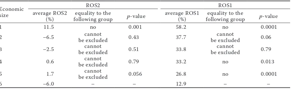
While, when comparing the mean ROS2 for the particular size categories, we cannot reject at the significance level α = 5% in the case of peripheral categories 2, 5, and 6 that the indicators for the re-maining categories are equal, in the case of indicator ROS1, its value differs besides size category 6 also in category 5 and nearly category 2. The subsidies

Table 6. Average ROS1 (returns on sales including subsidies) and ROS2 (returns on sales without subsidies and taxes), wheat yields and subsidies by the economic size of farms in 2004–2013

Economic size Average ROS1 (%) _{yields (100 kg/ha) Average ROS2 (%)}Average wheat _{yields (100 kg/ha)}Average wheat Average subsidies _(%)

1 58.2 35.8 11.5 35.8 46.7

2 37.7 40.6 –6.2 40.6 43.9

3 33.8 48.6 –2.5 48.6 36.3

4 33.2 53.6 0.6 53.6 32.6

5 26.8 55.9 1.7 55.9 25.1

6 12.9 62.4 –6.0 62.4 18.9

Source: authors‘ calculation based on FADN database (FADN 2016)

Table 7. Test on the equality of mean values of indicators ROS1 (returns on sales including subsidies) and ROS2 (re-turns on sales without subsidies and taxes)

Economic size

ROS2 ROS1

average ROS2

(%) following groupequality to the p-value average ROS1 (%) following groupequality to the p-value

1 11.5 no 0.001 58.2 no 0.0001

2 –6.5 _{be excluded}cannot 0.43 37.7 _{be excluded}cannot 0.06

3 –2.5 _{be excluded}cannot 0.51 33.8 _{be excluded}cannot 0.79

4 0.6 _{be excluded}cannot 0.79 33.2 no 0.013

5 1.7 _{be excluded}cannot 0.056 26.8 no 0.0001

6 –6.0 – – 12.9 – –

Source: authors‘ calculation based on FADN database (FADN 2016)

highlight the initial differences in the indicator ROS2. The difference between the indicators ROS1 and ROS2 (Table 6) shows that the largest share of subsidies in the EU, as regards the value of production, is re-ceived by the smallest farms. With a gradual growth

of the size category, subsidies decline in relation to the size of production. Thus, the subsidy policy prefers small farms. However, they reach the lowest yields per hectare. Their production is not even profitable at the level of ROS2 (applies to size categories 2–3; in case of size category 1, we can doubt that all produc-tion costs are included, such as the unpaid workforce of the family members).

Yields per hectare and the values of ROS2 (Table 6) by size category of the farms are captured in Figure 1. The monitored indicators in the chart show the dif-ferent status of the first size category. It reaches a completely different (the highest) indicator ROS2 at the lowest yields per hectare. In theory, the result indicates a low intensity of farming, which leads to lower yields per hectare, but saves the expense inputs, which in effect leads to the highest ROS2. It is also possible that these small economic units (Table 1) use the unpaid workforce more often (e.g. family members), which is not calculated in the profit or loss, thus increasing ROS2. The mentioned facts are worth further exploration.

Figure 1. Average ROS2 (returns on sales without subsi-dies and taxes ) and the wheat yields per ha with respect to the farm size category

Source: authors’ calculation based on FADN database (FADN 2016)

1 2 3

4 5 6

10.0 20.0 30.0 40.0 50.0 60.0 70.0

Wheat

yields

(100

kg/ha)

ROS2 (%)

–10 –5 0 5 10 15

0.0

Figure 2. Average ROS2 (returns on sales without subsi-dies and taxes) and the wheat yields per ha for farm size categories 4–6

y = ax + b is the estimated linear relationship between the values y (vertical axis) and x (horizontal axis) values. The coefficients a, b are estimated by the ordinary least squres method. R2 _{is the coefficient of determination}

Source: authors‘ calculation based on FADN database y = –14.909x + 53.7

R² = 0.3037 40.0 45.0 50.0 55.0 60.0

Wheat

yields

(100

kg/ha)

ROS2 (%) Size category 4

–30 –20 –10 0 10 20

y = –18.995x + 56.263 R² = 0.1316

40.0 45.0 50.0 55.0 60.0 65.0 70.0

Wheat

yields

(100

kg/ha)

ROS2 (%) Size category 5

–20 –10 0 10 20

y = –29.265x + 60.619

R² = 0.1701 _40.0 45.0 50.0 55.0 60.0 65.0 70.0 75.0

Wheat

yield

(100Kg/ha)

The negative gradient of the line fitted between the yields per hectare and ROS2 for the period 2004–2013 in all size categories of agricultural entities could indicate that an increase in wheat yields per hectare faces expense limits (additional yields are achieved at the cost of increased additional expenses). This relationship is the strongest in case of the biggest size categories (which also reach the greatest yields per hectare). The relationship between the indicator ROS2 and the wheat yields per hectare within size categories 4–6 is presented in Figure 2.

This result suggests that the entities in size cat-egory 6 primarily focus on the performance rat-ed by the volume of production (the effort for the highest possible yields per hectare), even at the cost of high expenses. However, the return on sales ROS1 is positive even in their case, so the reason can be the effort to reach a high turnover and thus a higher level of return on the capital invested.

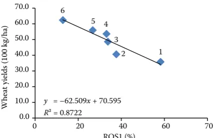
Figure 3. Average ROS1 (returns on sales including subsi-dies) and the wheat yields per ha with respect to the farm size category

y = ax + b is the estimated linear relationship between the values y (vertical axis) and x (horizontal axis) values. The coefficients a, b are estimated by the ordinary least squres method. R2 _{is the coefficient of determination}

Source: authors‘ calculation based on FADN database (FADN 2016)

1 2

3 4 5 6

y = –62.509x + 70.595 R² = 0.8722

0.0 10.0 20.0 30.0 40.0 50.0 60.0 70.0

Wheat

yields

(100

kg/ha)

ROS1 (%)

0 20 40 60 70

Figure 4. Average ROS1 (returns on sales including subsidies) and the wheat yields per ha for farm size categories 4–6

y = ax + b is the estimated linear relationship between the values y (vertical axis) and x (horizontal axis) values. The coefficients a, b are estimated by the ordinary least squres method. R2 _{is the coefficient of determination}

Source: authors‘ calculation based on FADN database (FADN 2016)

y = –32.272x + 64.312 R² = 0.4738

49.0 50.0 51.0 52.0 53.0 54.0 55.0 56.0 57.0 58.0 59.0

Wheat

yields

(10

0

kg/ha)

ROS1 (%) Size category 4

20 25 30 35 40 45

y = –47.704x + 68.71 R² = 0.2901

0.0 10.0 20.0 30.0 40.0 50.0 60.0 70.0

Wheat

yields

(10

0

kg/ha)

ROS1 (%) Size category 5

20 25 30 35

15

y = –52.243x + 69.12 R² = 0.3989

40.0 45.0 50.0 55.0 60.0 65.0 70.0 75.0 80.0

Wheat

yields

(10

0

kg/ha)

ROS1 (%) Size category 6

20 25 30

The progress of the indicator ROS2 starting from size category 2 up to category 6 could indicate an ideal size of an agricultural entity for wheat growing in respect to this indicator (size categories 4–5 reach positive ROS2).

It is obvious that the agricultural entities make decisions on the level of production, the intensity of farming, under a significant effect of the subsidies that the agricultural entities receive. Therefore, we evaluated the return on sales which included these subsidies and their relationship to wheat yields per hectare (Figure 3).

The results show that the smaller the farm is, the higher the return on sales and the lower the yields per hectare it achieves. The relationship between ROS1 and wheat yields per hectare is quite close (unlike the relationship between ROS2 and wheat yields per hectare (Figure1). This negative relationship between the return on sales and the wheat yields per hectare was found for all size categories. It was the strongest in categories 4, 5, and 6. The relationship within these categories is presented in Figure 4.

CONCLUSION

The results of the analysis demonstrate that the relationship between the profitability indicator return on sales and the volume of production measured by the wheat yields per hectare is ambiguous. Basically, there is a discordance in the progress of the volume of indicators of agricultural production, when the performance is understood as the ability to produce a certain amount of production from a unit of land, and the economic performance, which is measured by profit, i.e. the relation between the revenues and expenses and their mutual comparison. Since the ag-ricultural sector is a significant recipient of subsidies, the indicator return on sales (ROS) was used in two versions, ROS1, which includes subsidies, and ROS2, which excludes them. Subsidies can affect the value of the ROS in two ways, either in the form of the cost reduction, as the subsidies for the acquisition of fixed assets reduce their purchase prices and thus the value of depreciation, or in the form of the revenue increase when the operating subsidies are received.

The comparison of the wheat yields per hectare with ROS1 shows that the larger entities achieve higher yields per hectare, but the return on sales develops conversely – it declines with the growing size of the

difference among the size categories 1–6; the results in categories 2–5 fluctuate between increase and de-crease. The highest values are achieved in the size cat-egories 4–5 (so we can consider them the optimal size of a production unit for the wheat growing – a positive return on sales is reached without subsidies as well as the high yields per hectare). The high value of the return on sales in the size category 1 is achieved at a low yield per hectare. The reason may be a higher rate of the incomplete capturing of costs in case of small farms (e.g. the unpaid workforce of family members) and its higher significance in case of small farms. The low intensity of farming in case of small farms (which is in contrast to the phenomenon observed in developing countries (Cornia 1985)) can lead to an over-proportionate decrease in the cost inputs, which then leads to the positive return on sales. Lower yields per hectare of the smallest farms may be associated with worse access of the small businesses to finan-cial resources (Paseková 2005). This reduces their purchase of technology or hiring of skilled workers. It is possible that the larger entities, which have an easier access to financial resources, may spend more on the acquisition of inputs (or the acquisition of ag-ricultural investments) and achieve the intensification of agricultural production, which is then reflected in the shift from the negative values of ROS2 in case of size categories 2–3 to the positive values of ROS2 in the case of size categories 4–5. The answer to the question of rising yields per hectare in relation to the growth of the farm’s size category can also be the fact that the consolidation of agricultural entities was faster in the history in the areas more appropriate for agriculture (with naturally higher yields per hectare).

measured by yields per hectare) in order to increase the return on capital invested, although the intensity of farming is already so high that it is not any longer appropriate to keep it with regard to the cost inputs (excluding subsidies).

REFERENCES

Bijman J., Iliopoulos C., Poppe K.J., Gijselinckx C., Hage-dorn K., Hanisch M., Hendrikse G.W.J., Kühl R., Ollila P., Pyykkönen P., van der Sangen G. (2012): Support for Farmers‘ Cooperatives Final Report European Com-mission. “Support for Farmers’ Cooperatives (SFC)”. Available at http://ec.europa.eu/agriculture/external-studies/2012/support-farmers-coop/fulltext_en.pdf (accessed June 26, 2017).

Bohusova H., Svoboda P., Nerudova D. (2012): Biological assets reporting: Is the increase in value caused by the biological transformation revenue? Agricultural Eco-nomics – Czech, 58: 520–532.

Brierley J.A. (2016): An examination of the use of profit-ability analysis in manufacturing industry. International Journal of Accounting, Auditing and Performance Evalu-ation, 12: 85–102.

Cîrciumaru D., Siminica M., Marcu N. (2010): A study on the return on equity for the Romania industrial com-panies. Annals of the University of Craiova, Economic Sciences Series, 2: 1–8.

Cornia G.A. (1985): Farm size, land yields and the ag-ricultural production function. World Development, 13: 513–534.

Chrastinová Z. (2008): Economic differentiation in Slo-vak agriculture. Agricultural Economics – Czech, 54: 536–545.

Cucchiella F., D‘Adamo I., Gastaldi M. (2015): Financial analysis for investment and policy decisions in the re-newable energy sector. Clean Technologies, 17: 887–904. Eurostat (2016): National accounts and GDP. Available

at http://ec.europa.eu/eurostat/statistics-explained/ index.php/National_accounts_and_GDP/ (accessed June 26, 2017).

Farm Accountancy Data Network Database (FADN) (2016): Available at http://ec.europa.eu/agriculture/rica/data-base/database_en.cfm (accessed May 20, 2017). Golas Z. (2016): The level and determinants of work

prof-itability changes in the Czech and Polish agricultural sector in the years 2004–2014. Agricultural Economics – Czech, 62: 334–344.

Institute of Agricultural Economics of the Czech Republic (2016): Zpráva o stavu zemědělství ČR za rok 2015. Available at http://www.uzei.cz/data/usr_001_cz_soubo-ry/zzza2015vlada.pdf (accessed Apr 15, 2017).

Jedruchniewicz A., Danilowska A. (2016): Accuracy of economic situation projections in the Polish agriculture. Economic Science for Rural Development Conference Proceedings, 42: 228–234.

Miklovičová J., Gurčík L. (2009): The profit and added value creation and development analysis of agricultural companies in selected regions in Slovakia. Agricultural Economics – Czech, 55: 392–399.

Mishra A.K., Moss Ch.B., Erickson K.W. (2009): Regional differences in agricultural profitability, government payments, and farmland values: Implications of DuPont expansion. Agricultural Finance Review, 69: 49–66. Pasekova M. (2005): Mikroekonomicke aspekty

hospodar-eni malych a strednich podniku. E&M Economics and Management, 8: 6–12.

Sarris A.H., Doucha T., Mathijs E. (1999): Agricultural re-structuring in Central and Eastern Europe: implications for competitiveness and rural development. European Review of Agricultural Economics, 26: 305–329. Sedláček J. (2010): The methods of valuation in agricultural

accounting. Agricultural Economics – Czech, 56: 59–66. Svoboda J., Novotná M. (2011): Multifactor productivity

analysis in the sample of agricultural enterprises. Acta Universitatis Agriculturae et Silviculturae Mendelianae Brunensis, LIX, 7: 395–402.

Szymanska E.J. (2015): Profitability of pig farms in Poland after integration to the EU. Economic Science for Rural Development Conference Proceedings, 39: 97–107. Taeger D., Kuhnt S. (2014): Statistical Hypothesis Testing

with SAS and R. John Wiley & Sons, Ltd., Chichester. Věžník A., Svobodová H., Némethová J., Hradický J. (2017):

Livestock production in Czechia and Slovakia, ten years beyond EU accession. Human Geographies – Journal of Studies, 1: 77–93.

Vuckovic B., Veselinovic B., Drobnjakovic M. (2016): Analy-sis of profitability of selected agricultural enterprises in the Autonomous Province of Vojvodina, Republic of Serbia. Actual Problems of Economics, 176: 147–159. Záhorský T., Pokrivčák J. (2017): Assessment of the

ag-ricultural performance in Central and Eastern Euro-pean countries. Agris on-line Papers in Economics, 9: 113–123.