A Class of Momentum-Preserving Fourier Pseudo-Spectral Schemes for the Korteweg-de Vries Equation

A Class of Momentum-Preserving Fourier

Pseudo-Spectral Schemes for the Korteweg-de

Vries Equation

Jin-Liang Yan and Liang-Hong Zheng

Abstract—The invariant preserving is one of important

factors in designing numerical algorithms. The structure-preserving algorithms often have better stability and long time tracking ability than nonconservative schemes. In this paper, based on the bi-Hamiltonian structure of the wave equation, a class of momentum-preserving Fourier pseudo-spectral algo-rithms are proposed for the Korteweg-de Vries (KdV) equation. The proposed schemes can conserve the discrete momentum to machine precision, and have smaller phase and amplitude errors than the nonconservative scheme. At last, some examples are presented to validate the effectiveness of the proposed schemes.

Index Terms—Momentum; Bi-Hamiltonian systems; Fourier

Pseudo-Spectral method; KdV equation

I. INTRODUCTION

I

ut+εuux+µuxxx= 0, (1)

where ε and µ are given constants. The KdV equation [1] is a nonlinear partial differential equation (PDE), which was originally described the propagation of a solitary wave on the water surface. The KdV equation is one of the simplest mod-els featuring nonlinear convection (the term uux) and linear dispersion (the higher-order termuxxx) [2]. The interaction of the dispersion term and the nonlinear term will produce permanent and localized wave forms; This phenomenon was first observed numerically by Zabusky and Kruskal (1965) [3], long after John Scott Russell’s experimental observation of solitons in 1834.

The KdV equation is a completely integrable equation [4], and has an infinite number of conservation laws [5], the first

Manuscript received April 18, 2019; revised July 22, 2019. This work was supported in part by the National Natural Science of China(Grant NO. 11861047), Foundation Jiangsu Key Laboratory for NSLSCS (Grant No. 201804), PhD Start-up Fund of Wuyi University (Grant No. YJ201702), the Education Foundation of Fujian Province for Young Teachers(Grant No. JA14319, NO. JAT160519), Natural Science Foundation of Fujian Province(Grant No. 2016J01682).

Jin-Liang Yan is with the department of Mathematics and Computer, Wuyi University, Wuyi Shan, Fujian, 354300, China, e-mail: yanjin-liang3333@163.com.

Liang-Hong Zheng is with the department of Information and Computer Technology, No 1 middle school of Nanping, Nanping, Fujian, 353000, China. e-mail: 413845939@qq.com.

three conservation laws are

M=

Z b

a u dx,

K= 1 2

Z b

a u2dx,

H= Z b

a

−1

6εu

3₊1

2µu

2 x

dx,

which are respectively named mass, momentum and energy. In scientific research, it is often difficult or even impossible to obtain the exact solution of the nonlinear equation. Thus, we often have to resort to numerical simulation [6]–[8]. The numerical simulations of the KdV equation can capture a series of interesting wave phenomena, such as solitary wave, the interaction of two solitary waves, and so on. Many numerical methods have been used to solve the KdV equation, such as finite difference methods [9]–[11], finite element methods [12]–[14], finite volume methods [15], [16], spectral methods [17]–[19], and discontinuous Galerkin methods [20]–[22], and so on.

Numerous theoretical and experimental results show that the structure-preserving algorithms often have good numer-ical properties, i.e., the excellent long-time behavior, the linear error growth, and smaller amplitude and phase errors, and so on. In the spirit of structure-preserving algorithms, a good numerical method should preserve the physical quantities underlying the partial differential equations as far as possible. This presents a challenge for accurate and efficient numerical simulations, as the proposed schemes should conserve the invariants of the KdV equation as soon as possible. Researchers have proposed many structure-preserving algorithms for the KdV equation. For example, symplectic algorithms [23], energy-preserving algorithms [20], [22], [24], and the momentum-preserving algorithms [2], [21], [25], and so on.

In fact, the KdV equation is a bi-Hamiltonian system. On the one hand, the KdV equation is a Hamiltonian PDE [26], i.e., it can be written as

∂u ∂t =J

δH

δu, H= Z b

a

−1

6εu

3₊1

2µu

2 x

dx, (2)

where J = ∂x is a skew-symmetric operator, and δ_δuH = ∂H

∂u − ∂ ∂x

∂H

∂ux

denotes the variational derivative of H with respect to u. Based on the above property, different sym-plectic algorithms and energy-preserving algorithms can be designed.

IAENG International Journal of Applied Mathematics, 49:4, IJAM_49_4_22

On the other hand, the KdV equation can also be refor-mulated as another Hamiltonian form [27],

∂u

∂t =N(u) _δK

δu

, K= 1 2

Z b

a

u2_{dx, (3)} whereN(u) =−(∂2

x+23u∂x+ 1

3∂xu)is a linear and anti-symmetric operator. Based on the above property, we can construct various momentum-preserving algorithms.

The focus of the present paper is on the momentum-preserving schemes, which is based on the second Hamil-tonian system, i.e., Eq. (3). To our knowledge, the scheme has been considered in the context of multi-symplectic PDEs in [28]. It is shown that this scheme exactly preserves the local momentum, as well as multi-symplectic conservation law. In addition, Bona et al. [2] constructed a class of con-servative discontinuous Galerkin schemes for the generalized Korteweg-de Vries equation. The schemes can precisely con-serve the discrete mass and momentum. Liu [21] proposed a direct discontinuous Galerkin method based on the second Hamiltonian system of the KdV equation.

In this paper, we shall construct two high-order momentum-preserving schemes based on the Eq. (3). We first approximated the spatial derivative of the KdV equation by using the Fourier pseudo-spectral method, and obtain a semi-discretized system, which can exactly conserve the semi-discrete momentum. Subsequently, two second-order accurate finite difference methods are employed to discretize the resulting ordinary differential equations (ODEs) and two fully discrete momentum-preserving schemes are derived.

In this paper, we will investigate the effectiveness of the proposed schemes, in particular discretization errors, wave amplitude, and phase errors are discussed. The results demonstrate that the conservative properties of the numerical methods could be critical in obtaining the long time behavior of the solutions.

The paper is organized as follows. In Section2.1, we first approximate the spatial derivatives of the KdV equation by the Fourier pseudo-spectral method and obtain corresponding semi-discrete scheme. Then in Section2.2, we discretize the above semi-discretized system using two second-order accu-rate finite difference methods. In Section3, we investigate the conservative properties of the semi-discrete scheme and the fully discrete schemes. Finally, in Section4, some examples are presented to validate the effectiveness of the proposed schemes.

II. MOMENTUM-PRESERVINGFOURIER PSEUDO-SPECTRAL METHODS

In this section, the momentum-preserving Fourier pseudo-spectral methods are proposed for the following KdV equa-tion

ut=−εuux−µuxxx, (4) subject to periodic boundary condition

u(a, t) =u(b, t),

whereu(x, t)is the exact solution of (4), andε,µ,a andb are constants.

Eq. (4) can be rewritten as the following Hamiltonian form ut=N(u)

δK

δu, N(u) =− ε

3(u∂x+∂xu)−µ∂xxx, (5)

where N(u) is a skew-symmetric operator. Eq.(5) satisfies the following momentum conservation law

dK

dt = 0, i.e.,K=C. In fact,

˙

K= (∇K)T_{u˙ = (∇K)}T_{N(u)∇K= 0,}

where∇K denotes the gradient of K and u˙ represents the derivative ofuwith respect tot.

A. Space discretization

In this paper, we consider the KdV equation (5) over the intervalI= [a, b], andxj =a+jh, (j = 0,1, . . . , M−1) denote the mesh nodes,h= (b−a)/M represents the spatial step, and M is a even number. In the following, let u = (u0, u1, . . . , uM−1)T, and ui (0≤i≤M −1) denotes the approximation tou(xi, t).

The crucial step of the Fourier pseudo-spectral method is to approximate the partial differential operators. From [29], we know that the first-order partial differential operator∂x yields the Fourier spectral differential matrixD1, the second-order partial differential operator ∂xx yields the Fourier spectral differential matrixD2. HereD1 is aM×M skew-symmetric matrix with elements

(D1)m,n=

(₁

2(−1)m+ncot(ω xm−xn

2 ), m6=n,

0, m=n. (6)

andD2 is aM×M symmetric matrix with elements

(D2)m,n=

(₁

2ω

2₍₋₁₎m+n+1 1 sin2_(ωxm−xn

2 )

, m6=n,

−ω2M2₊₂

12 , m=n.

(7)

In particular, the partial differential operatorsuxanduxxx are respectively approximated byD1uandD₃u. Therefore,

we have the following semi-discrete scheme du

dt =N(u) δK

δu,

(8) whereN(u) =−ε

3(diag(u)D1+D1diag(u))−µD₃, and

K=h 2u

T_u.

It is clearly seen thatK is also conservative after spatial semi-discretization. In fact, by (8), we have

du

dt =JM∇K(u), JM =

1

hN(u), (9) where N(u) is a skew-symmetric matrix, i.e., N(u)T = −N(u). Thus

d

dtK(u) =∇K(u)

T_u′_{(t) =∇K(u)}T_{N(u)∇K(u) = 0.}

B. Time discretization

We now turn to time discretization of Eq. (8). Denotetn= nτ,Ω∆t={tn|0 ≤n≤N},∆t=T /N denotes the time step, andNis a positive integer. SupposeU ={Un_|0≤n≤ N} is a grid function onΩ∆t. For convenience, introducing the following notations:

tn+1/2= 1 2(t

n_+tn+1_{), U}n,1₌ 1

3(U

n+1_+Un_+Un−1_),

Un+1/2=1 2(U

n_+Un+1_{), U}n,2₌1

2(U

n+1/2_+Un−1/2_).

IAENG International Journal of Applied Mathematics, 49:4, IJAM_49_4_22

Firstly, we employ the leap-frog scheme, and N(u) is approximated byN(Un,1),

Un+1_−Un−1

2∆t =N(U n,1

)U

n+1_+Un−1

2 , (10)

wheren= 1,2, . . . , T /∆t.

On the other hand, ifN(u)is approximated byUn,2, we have

Un+1_−Un−1

2∆t =N(U n,2

)U

n+1/2_+Un−1/2

2 , (11)

wheren= 1,2, . . . , T /∆t.

Remark II.1. In what follows, for convenience, the first

scheme is named CMFPM1 and the second one is named CMFPM2.

Remark II.2. The CMFPM1 and the CMFPM2 are two

three-level momentum-preserving schemes. The initial value U1 _{is approximated by the the following} momentum-preserving scheme

U1_−U0

∆t =J2(U

0₎U0+U1

2 . (12)

III. CONSERVATIVE PROPERTY OF THE PROPOSED SCHEMES

In this section, we analyze the conservative properties of the CMFPM1 and the CMFPM2.

Theorem III.1. Let Un be the solution of the scheme (10) and (12), and assume it satisfies the periodic boundary condition, then the solution of the scheme (10) satisfies

K(Un) =K(U0), K(Un)≈1 2

M

X

k=0

(Ukn)2h, (13)

wheren= 1,2, . . . , T /∆t.

Proof: By computing theL2 _{inner product of (12) with}

(U0_+U1_{)/2, we have} U1_−U0

∆t ,

U0_+U1

2

= N(U0)U

0_+U1

2 ,

U0_+U1

2

,

whereN(U0_{)is aM×M skew-symmetric matrix, thus}

1 ∆t(K(U

1_)−K(U0_{)) =} U0+U1

2 T

N(U0)U

0_+U1

2 = 0,

then

K(U1) =K(U0).

Similarly, by computing the L2 _{inner product of (10) with}

(Un+1_+Un−1_{)/2, we have} Un+1_−Un−1

2∆t ,

Un+1_+Un−1

2

= N(Un,1)U

n+1_+Un−1

2 ,

Un+1_+Un−1

2

,

whereN(Un,1)is aM×M skew-symmetric matrix, thus

1 2τ(K(U

n+1_)−K(Un−1₎₎

= U

n+1_+Un−1

2

T

N(Un,1)U

n+1_+Un−1

2 = 0,

Therefore,

K(Un) =K(U0), n= 1,2, . . . , T /∆t−1.

Theorem III.2. Let Un+1/2 _{be the solution of the scheme} (11) and (12), and assume it satisfies the periodic boundary condition, then the solution of the scheme (11) satisfies

K(Un+1/2)≡K(U1/2), K(Un+1/2)≈h 2

M

X

k=0

(U_kn+1/2)2,

wheren= 1,2, . . . , T /∆t−1.

Proof: By computing theL2_{inner product of (11) with}

(Un+1/2_+Un−1/2_{)/2, we have} Un+1/2_−Un−1/2

∆t ,

Un+1/2_+Un−1/2

2

= N(Un,2)U

n+1/2_+Un−1/2

2 ,

Un+1/2_+Un−1/2

2

,

whereN(Un,2)is aM ×M skew-symmetric matrix, thus

1 ∆t(K(U

n+1/2_)−K(Un−1/2₎₎

= U

n+1/2_+Un−1/2

2

T

N(Un,2)U

n+1/2_+Un−1/2

2 = 0.

Thus,

K(Un+1/2) =K(U1/2), n= 1,2, . . . , T /∆t−1.

IV. NUMERICAL EXPERIMENTS

In this section, we will consider the following five test problems: the propagation of a single solitary wave (see Figure 7), the interaction of two solitary waves (see Figure 11), the interaction of five solitary waves (see Figure 13), the Zabusky-Kruskal’s problem (see Figure 15), and the linear KdV equation (see Figure 18). Through these numerical examples, we show that the proposed schemes are effective in simulating the KdV equation, and that they can precisely conserve the discrete momentum.

A. Example 1

In this example, we consider the following initial value problem

ut+uux+µuxxx= 0, x∈[0,1], t >0, u(x,0) =u0(x), x∈[0,1],

(14) subject to periodic boundary conditions. Eq. (14) has the following cnoidal-wave solution,

u(x, t) =Acn2(4W(m)(x−vt−x0)), (15) wherecn(z:m)is the Jacobi elliptic function with modulus m = 0.9,A = 192mµW2_{(m), v = 64µ(2m−1)W}2_(m), and x0 = 1/2. Here, the function W(m) is the complete elliptic integral of the first kind. It is worth noting that the cnoidal-waves is a kind of stable solutions of the time dependent problem [30], so numerical errors will not lead to instabilities of the continuous problem. Thus, any insta-bility that appears is caused by the numerical scheme. This example is derived from [2].

Let{Un

j|0≤j ≤M −1,0≤n≤N} be the numerical solution of the proposed schemes andu(xj, tn)be the exact solution at node(xj, tn). In order to estimate the error and

IAENG International Journal of Applied Mathematics, 49:4, IJAM_49_4_22

convergence order of the proposed schemes, we define the following error norms

L1= M−1

X

j=0

|Ujn−u(xi, tn)|h,

L2=

M−1 X

j=0

|Ujn−u(xi, tn)|2h

1/2 ,

L∞= max

0≤j≤M−1|U n

j −u(xi, tn)|, and convergence order

order=log2

kU2h−uk

kUh−uk .

On the other hand, in order to measure the conservative properties of the proposed schemes, the discrete invariants and corresponding relative errors are respectively defined as

M(U(n)) =h M−1

X

k=0 U_k(n),

K(U(n)_{) =}h

2

M−1

X

k=0

(U_k(n))2_,

H(U(n)) =h M−1

X

k=0

−ε

6(U

(n) k )

3₊µ

2U

(n) k (D2U

(n)₎ k,

relative error=log10

|In i −Ii0|

|I0 i|

.

In the following, unless we specify otherwise,µ= 1/242_, and computational domain is divided into M cells. To measure the orders of convergence in time, we compute the numerical solutions with four different time step sizes

∆t = 0.1,0.05,0.025,0.0125 and spatial step is chosen as h = 1/200. This choice guarantees that the discretization error in spatial direction can be neglected. The results are presented in Tables I and III. The results show that the convergence of the proposed schemes are second order as expected. In addition, it is noted that the relative errors of the mass and energy are also second order accuracy, which is displayed in Figure 1.

10−5 10−4 10−3

10−10 10−8 10−6 10−4 10−2

∆ t

L∞

errors of invariants

CMFPM1 mass CMFPM1 energy CMFPM2 mass CMFPM2 energy y=2x

Fig. 1: The relative errors of the invariants versus time step. On the other hand, in order to measure the error in spatial direction, the time step size is chosen to be ∆t =1.0e-05, such that the discretization error in time direction can be neglected. The results are presented in Tables II and IV. It is

observed that the proposed schemes reach spectral accuracy in spatial direction, as expected.

We compare the proposed methods with the momentum-preserving methods within references in terms of accuracy. Table V shows that the L2-errors of different methods at t= 10. It is observed that the proposed methods have smaller errors than the implicit midpoint discontinuous Galerkin method (IMDGM) in [2] and Crank-Nicholson discontinuous Galerkin method (CNDGM) in [21] for k = 3, and the proposed methods have larger errors than the schemes in [25]. On the other hand, it is also noted that the CMFPM2 has smaller errors than the CMFPM1.

We now verify the conservative property of the proposed methods, and compare it with a non-conservative Fourier pseudo-spectral method (NCMFPM). Here, for convenience, we consider the implicit Euler method for the time discretiza-tion. The implicit Euler method, though only first order in time, is easy to implement in simulating various wave patterns and is also a non-conservative method. By resorting to it, we derive the following NCMFPM,

Un+1_−Un

∆t =−

η

2D1(U

n+1₎2_−µD 3Un+1,

whereD1 andD3 are Fourier differential matrices.

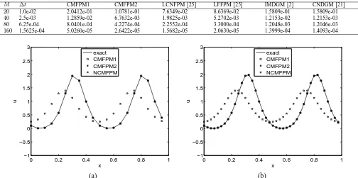
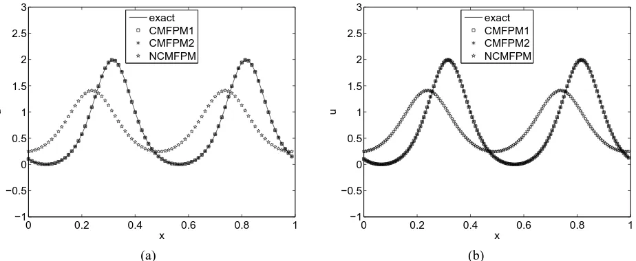
We start with the cnoidal-waves test problem with∆t= 0.001andM = 20,40,80,160. Fig.2 and Fig.3 compare the numerical solutions of three proposed methods att= 20. The exact solution is provided as a reference in the plots. It is clearly seen that the NCMFPM has a large phase errors, and both CMFPM1 and CMFPM2 makes a good approximation to the exact solution. Besides the large phase error, the amplitude of the wave produced by the NCMFPM decays as time increases. As is shown in Fig. 6b, the relative error of the momentum of the CMFPM1 is about 10−14_{, 10}−8 for the CMFPM2, and 10−1 _{for the NCMFPM. Thus, if} the momentum is not conserved, the amplitude of the wave decrease with time. Fig. 5 presents the time evolution of theL∞-error. It shows that theL∞-error of the conservative

methods have smaller errors. Indeed, at timet= 20, the error of the NCMFPM is about297times larger than the proposed methods, and the L∞-errors of the proposed methods grow

linearly with time.

We also evaluate the long time behavior of the proposed schemes. To this end, we set M = 80, time step ∆t = 0.001, and the computation is done up to timet= 1000. The numerical solutions of the proposed schemes are presented in Fig. 7 and Fig. 8. The exact solution is also provided as a reference in the plot. It is found that both methods make a good approximation to the exact solution. The L∞-error

and the relative errors of three invariants are presented in Fig. 9 and Fig. 10. As is shown in Fig. 9b and Fig. 10, the relative errors of the mass is about6×10−6_{; the momentum} is exactly conserved for the CMFPM1, and2×10−8_{for the} CMFPM2; the energy is about3×10−5_{for the CMFPM1 and} the CMFPM2. From Fig. 9a, it is noted that theL∞-error of

the proposed methods increase linearly with time. This may reflect the fact that all the solitons travel with well-preserved shape and thus the principle part of the numerical error is the phase error [22].

IAENG International Journal of Applied Mathematics, 49:4, IJAM_49_4_22

TABLE I: TheL1,L2 andL∞ errors and convergence orders in time for the CMFPM1.

∆_{t L}1 order L2 order L∞ order

1_/20 _{3.7380e-01 — 4.4000e-01 — 7.9010e-01 —}

1/40 1.0240e-01 1.8681 1.2290e-01 1.8400 2.1990e-01 1.8452 1_/80 2.7100e-02 1_.9179 3.2100e-02 1_.9368 5.5200e-02 1_.9941 1/160 6.7000e-03 2.0161 8.1000e-03 1.9866 1.4200e-02 1.9588 1_/320 1.7000e-03 1_.9786 2.0000e-03 2_.0179 3.7000e-03 1_.9403

TABLE II: TheL1,L2 andL∞ errors and convergence orders in space for the CMFPM1.

h L1 order L2 order L∞ order

1/10 5.5156e-04 — 6.3062e-04 — 8.7247e-04 —

1_/20 1.1485e-05 5.5857 1.3227e-05 5.5752 2.1849e-05 5.3195

1/40 2.0793e-08 9.1094 2.4137e-08 9.0980 4.2917e-08 8.9918

TABLE III: TheL1,L2andL∞errors and convergence orders in time for the CMFPM2.

∆t L1 order L2 order L∞ order

1_/20 2.0930e-01 — 2.4200e-01 — 4.0720e-01 —

1_/40 _{5.6500e-02 1.8892 6.4100e-02} 1_.9166 _1.0610e-01 1_.9403 1_/80 1.4100e-02 2.0026 1.6200e-02 1_.9843 2.6500e-02 2_.0014 1_/160 _{3.5000e-03 2.0103 4.1000e-03} 1_.9823 _7.1000e-03 1_.9001 1/320 8.8524e-04 1.9832 1.0000e-03 2.0356 1.8000e-03 1.9798

TABLE IV: TheL1,L2 andL∞ errors and convergence orders in space for the CMFPM2.

h L1 order L2 order L∞ order

1_/10 _{5.5156e-04 — 6.3062e-04 — 8.7247e-04 —}

1/20 1.1485e-05 5.5857 1.3227e-05 5.5752 2.1849e-05 5.3195

1_/40 _{2.0791e-08 9.1096 2.4142e-08 9.0977 4.3361e-08 8.9770}

TABLE V: L2-errors of the numerical solutions obtained from the different methods for the cnoidal-wave problem; comparisons with the exact solution at timet= 10.

M ∆t CMFPM1 CMFPM2 LCNFPM [25] LFFPM [25] IMDGM [2] CNDGM [21]

20 1.0e-02 2.0412e-01 1.0781e-01 7.6349e-02 8.6369e-02 1.5809e-01 1.5809e-01 40 _{2.5e-03 1.2859e-02 6.7632e-03 1.9825e-03 5.2702e-03 1.2153e-02 1.2153e-03} 80 _{6.25e-04 8.0401e-04 4.2274e-04 2.2552e-04 3.3000e-04 1.2048e-03 1.2046e-03} 160 1.5625e-04 5.0260e-05 2.6422e-05 1.5682e-05 2.0630e-05 1.3999e-04 1.4093e-04

0 0.2 0.4 0.6 0.8 1

−1 −0.5 0 0.5 1 1.5 2 2.5 3

x

u

exact CMFPM1 CMFPM2 NCMFPM

0 0.2 0.4 0.6 0.8 1

−1 −0.5 0 0.5 1 1.5 2 2.5 3

x

u

exact CMFPM1 CMFPM2 NCMFPM

(a) (b)

Fig. 2: Numerical approximations of the cnoidal-wave problem using the CMFPM1, CMFPM2, and NCMFPM; comparisons with the exact solution at timet= 20with∆t= 0.001.(a)20uniform elements,(b)40uniform elements.

B. Example 2

In this example, we consider again the KdV equation with ε = 1, µ = 1. The KdV equation has the following two

solitary waves

u(x, t) = 12

(1 +eθ_1+eθ_2+a2_eθ₁+θ₂₎2[k 2

1eθ1+k22eθ2+

2(k2−k1)2eθ1+θ2+a2(k22eθ1+k21eθ2)eθ1+θ2],

(16) wherea2₌ k₁−k₂

k1+k2 2

= 1

25,θ1=k1x−k 3

1t+x1,θ2=k2x− k3

2t+x2. In the following, we setk1= 0.4,k2= 0.6,x1= 4,

IAENG International Journal of Applied Mathematics, 49:4, IJAM_49_4_22

0 0.2 0.4 0.6 0.8 1 −1

−0.5 0 0.5 1 1.5 2 2.5 3

x

u

exact CMFPM1 CMFPM2 NCMFPM

0 0.2 0.4 0.6 0.8 1

−1 −0.5 0 0.5 1 1.5 2 2.5 3

x

u

exact CMFPM1 CMFPM2 NCMFPM

(a) (b)

Fig. 3: Numerical approximations of the cnoidal-wave problem using the CMFPM1, CMFPM2, and NCMFPM; comparisons with the exact solution at timet= 20with∆t= 0.001.(a)80uniform elements,(b)160uniform elements.

0 5 10 15 20

0 0.5 1 1.5 2

t L ∞

error

CMFPM1 CMFPM2 NCMFPM

0 50 100 150 200

0 0.5 1 1.5 2

t L ∞

error

CMFPM1 CMFPM2 CMFPM3 NCMFPM

(a) (b)

Fig. 5: Time history of theL∞-error of the numerical approximations obtained from the CMFPM1, CMFPM2, and NCMFPM

for the cnoidal-wave problem with∆t= 0.001and a uniform mesh with 80elements.(a) t=20,(b) t=200.

0 50 100 150 200

10−6 10−4 10−2 100 102

t

relative error of energy

CMFPM1 CMFPM2 NCMFPM

0 50 100 150 200

10−15 10−10 10−5 100

t

relative error of momentum

CMFPM1 CMFPM2 NCMFPM

(a) (b)

Fig. 6: Time history of the relative errors of the invariants obtained from the CMFPM1, CMFPM2, and NCMFPM with

∆t= 0.001and80uniform elements. (a) energy,(b) momentum.

x2= 15, and the solution region is chosen as[−40,40]. The above solution represents a two solitary waves, i.e., a tall

solitary wave and a short one, both solitary waves travel from left to right at a constant speed, and the speed of the

IAENG International Journal of Applied Mathematics, 49:4, IJAM_49_4_22

0 0.2 0.4 0.6 0.8 1 0

0.5 1 1.5 2

x

u

Exact CMFPM1 CMFPM2

0 0.2 0.4 0.6 0.8 1

0 0.5 1 1.5 2

x

u

Exact CMFPM1 CMFPM2

(a) (b)

Fig. 7: Numerical solutions att= 0,200with∆t= 0.001and80uniform elements. (a)t= 0,(b)t= 200.

0 0.2 0.4 0.6 0.8 1

0 0.5 1 1.5 2

x

u

Exact CMFPM1 CMFPM2

0 0.2 0.4 0.6 0.8 1

0 0.5 1 1.5 2

x

u

Exact CMFPM1 CMFPM2

(a) (b)

Fig. 8: Numerical solutions att= 500 and1000with∆t= 0.001and80 uniform elements. (a)t= 500,(b)t= 1000.

0 200 400 600 800 1000

0 0.05 0.1 0.15 0.2 0.25 0.3 0.35

t L∞

error

CMFPM1 CMFPM2

0 200 400 600 800 1000

0 0.2 0.4 0.6 0.8 1 1.2 1.4x 10

−5

t

mass error

CMFPM1 CMFPM2

(a) (b)

Fig. 9: Time history of theL∞-error, the relative errors of the mass using the CMFPM1 and the CMFPM2 with∆t= 0.001

and80uniform elements. (a) L2_{-errors,(b) mass errors.}

tall one is bigger than the short one.

For computation, we set M = 160, time step ∆t = 0.1,

and the computation is done up to time t = 120. The numerical solutions at four different times are presented in

IAENG International Journal of Applied Mathematics, 49:4, IJAM_49_4_22

0 200 400 600 800 1000 0

0.5 1 1.5 2 2.5 3 3.5 4 4.5x 10

−8

t

momentum error

CMFPM1 CMFPM2

0 200 400 600 800 1000

0 1 2 3 4 5 6 7 8 9x 10

−5

t

energy error

CMFPM1 CMFPM2

(a) (b)

Fig. 10: The relative errors of the momentum and energy using the CMFPM1 and the CMFPM2 with∆t= 0.001and80

uniform elements. (a) momentum errors,(b) energy errors.

−400 −20 0 20 40

0.2 0.4 0.6 0.8 1 1.2 1.4

x

u

exact CMFPM1 CMFPM2

−40 −20 0 20 40

−0.2 0 0.2 0.4 0.6 0.8 1

x

u

exact CMFPM1 CMFPM2

(a) (b)

Fig. 11: Numerical solutions att= 0andt= 60with∆t= 0.1and160uniform elements.(a)t= 0,(b)t= 60.

0 0.2 0.4 0.6 0.8 1

−1 −0.5 0 0.5 1 1.5 2 2.5 3

x

u

exact CMFPM1 CMFPM2 NCMFPM

Fig. 4: Numerical solutions of the cnoidal-wave problem using the CMFPM1, CMFPM2, and NCMFPM; comparisons with the exact solution at timet= 200.

Fig. 11 and Fig. 12. The exact solution is provided as a reference in the plots. The plots show that the numerical solutions agree quite well with the exact solution. As is shown in Fig. 11 and Fig. 12, at t= 0, the tall one located

on the left of the short one, at t= 60, the tall one catches up the short one, at t = 80, the tall one and the short one overlap together, and att = 120, the tall one and the short one exchange the positions.

C. Example 3

In this example, we consider the KdV equation (1) with ε = 1 and µ = 1 over the interval [−150,150]. It has the following initial condition

u(x,0) =

5

X

i=1

12k2isech 2

(ki(x−xi)), (17)

whereki,xi are constants.

k1= 0.3, k2= 0.25, k3= 0.2, k3= 0.2, k4= 0.15, k5= 0.1, x1=−120, x2=−90, x3=−60, x4=−30, x5= 0.

and adopt the periodic boundary condition. This example is derived from [14]. Here, for computation, setk1 = 0.3, k2 = 0.25, k3 = 0.2, k3 = 0.2, k4 = 0.15, k5 = 0.1, x1 = −120, x2 = −90, x3 = −60, x4 = −30, x5 = 0,

IAENG International Journal of Applied Mathematics, 49:4, IJAM_49_4_22

−40 −20 0 20 40 −0.1

0 0.1 0.2 0.3 0.4 0.5 0.6 0.7 0.8

x

u

exact CMFPM1 CMFPM2

−40 −20 0 20 40

−0.2 0 0.2 0.4 0.6 0.8 1 1.2

x

u

exact CMFPM1 CMFPM2

(a) (b)

Fig. 12: Numerical solutions att= 80andt= 120with∆t= 0.1 and160uniform elements. (a) t= 80,(b)t= 120.

0 100 200 300 400 500 600

0 1 2 3 4

5x 10

−7

t

momentum error

CMFPM1 CMFPM2

Fig. 14: The relative errors of momentum.

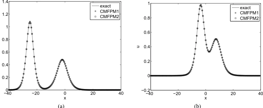
M = 256, and ∆t = 0.02. The numerical solution of the CMFPM1 is presented in Fig. 13a. The initial solution and the numerical solution of CMFPM1 at t = 600 are presented in Fig. 13b. It shows that the wave with taller amplitude travels faster than the other waves, and the shape and the amplitude are preserved very well at the final time. We believe that the conservative properties of the proposed schemes play a critical roles. Indeed, as illustrated in Fig. 14, the CMFPM1 can exactly conserve the discrete momentum to machine precision, and the CMFPM2 to 5×10−7_.

D. Example 4

Like in the pioneering paper [3], we consider the KdV equation with µ= 0.0222_{in the periodic domain[0,2], and} assume the following initial condition

u(x,0) = cos (πx),

The solution starts with a cosine wave and latter on develops a train of 8 solitons, which travel at different speeds and interact with each other, see [3] for detailed description of the solution. This example is derived from [24]. According to [24], there are several critical moments in the development of the solution: (i)t=tB = π1, the so-called breakdown time, (ii) t = 3.6tB, a train of 8 solitons have been developed, (iii) t = 0.5tR, wheretR = 30.4tB, all the odd-numbered

solitons overlap at x = 0.385 and all the even-numbered ones overlap atx = 1.385, and (iv) t =tR = 30.4tB, the so-called recurrence time, at which one expects to recover the initial condition. In the following test, we setM = 200and

∆t = 0.005

π . The numerical solution of the CMFPM1 over t∈[0,3.6tB]is displayed in Fig. 15a, from which we clearly see8solitons. In Fig. 15b, we show the numerical solutions at different critical times. The plot shows that, at timetB, the solution start to breakdown and at timet= 3.6tB, we discern a train of8solitons. These results are in well agreement with the ones of [24], [31].

As in [24], [31], we then carry out the computation up to the time 0.5tR, tR, 2tR, 5tR, 10tR and 20tR. The results are presented in Fig. 16. It is shown that these numerical solutions are smooth and stable, since no spurious oscillation are observed in the solution. Our results are agree quite well with the ones of [31], but differ from the ones of [24] after 10tR. On the other hand, to show the interactions of solitons in the solution, we display the (x-t)-contour plots of the numerical solutions in the time interval [0, tR] and

[19tR,20tR]in Fig. 17.

E. Example 5

In this example, we consider the following linear KdV equation

 



ut−ux+uxxx= 0, 0≤x≤2π, t >0, u(x,0) = sin (x), 0≤x≤2π,

u(0, t) =u(2π, t), t >0,

which has the following exact solution u(x, t) = sin (x+ 2t).

Firstly, we use this solution to check the accuracy and con-vergence rate of the proposed methods. To obtain the order of convergence in time, set ∆t= 1/5,1/10,1/20,1/40,1/80, h= 1/160, and the computation is done up to timet = 1. The numerical errors and the order of convergence are presented in Tables VI and VII. The results show that the proposed methods achieves second order accuracy in time, as expected.

Secondly, we use this solution to check the long time behavior and the conservative properties of the proposed

IAENG International Journal of Applied Mathematics, 49:4, IJAM_49_4_22

0 120 240 360 480 600

150 75

0 −75 −150 0

0.5 1 1.5

x t

U

−150 −100 −50 0 50 100 150

−0.5 0 0.5 1 1.5 2 2.5 3

x

u

u(x,0) CMFPM1

(a) (b)

Fig. 13: Interaction of five solitary waves for the CMFPM1 with∆t= 0.02and256uniform elements.(a) numerical solution over [0,600],(b)t= 600.

0 0.191 0.382 0.573 0.764 0.955 1.146

2 1.6 1.2 0.8 0.4 0 −1

−0.5 0 0.5 1 1.5 2 2.5

x t

U

0 0.5 1 1.5 2

−1 0 1 2 3 4 5 6 7

x

u

t=0 t=t

B

t=3.6t_B

(a) (b)

Fig. 15: Numerical solutions of the CMFPM1 with∆t= 0.005/π and200uniform elements. (a) numerical solution over

[0,3.6tB],(b) numerical solutions at t= 0, tB and3.6tB≈1.1459.

0 0.5 1 1.5 2

−1 −0.5 0 0.5 1 1.5 2

x

u

t=0.5t_R

t=t R t=2t R

0 0.5 1 1.5 2

−1 −0.5 0 0.5 1 1.5 2 2.5

x

u

t=5t_R

t=10t R t=20t

R

(a) (b)

Fig. 16: Numerical solutions of the CMFPM1 with ∆t = 0.005/π and 200uniform elements. (a) t = 0.5tR, tR,2tR,(b)

5tR,10tR and20tR.

methods. To this end, set M = 40, ∆t =2.5e-03, and the computation is done up to time t = 1000. The numerical

IAENG International Journal of Applied Mathematics, 49:4, IJAM_49_4_22

x

t

0 0.5 1 1.5 2

0 2 4 6 8 10

x

t

0 0.5 1 1.5 2

184 186 188 190 192 194

(a) (b)

Fig. 17: Contour plots of the numerical solutions in the(x, t)-plane. (a)t∈[0, tR],(b)t∈[19tR,20tR]. TABLE VI: The L1,L2 andL∞ errors and convergence orders in time for the CMFPM1.

∆_{t L}1 order L2 order L∞ order

1_/5 _{3.3260e-01 — 1.4740e-01 — 8.3200e-02 —}

1/10 1.0420e-01 1.6744 4.6200e-02 1.6738 2.6000e-02 1.6781 1_/20 2.6500e-02 1_.9753 1.1700e-02 1_.9814 6.6000e-03 1_.9780 1/40 6.7000e-03 1.9838 2.9000e-03 2.0124 1.7000e-03 1.9569 1_/80 1.7000e-03 1_.9786 7.3825e-04 1_.9739 4.1651e-04 2_.0291

TABLE VII: TheL1,L2 andL∞errors and convergence orders in time for the CMFPM2.

∆t L1 order L2 order L∞ order

1/5 1.0420e-01 — 4.6200e-02 — 2.6000e-02 —

1_/10 2.6500e-02 1_.9753 1.1700e-02 1_.9814 6.6000e-03 1_.9780 1/20 6.7000e-03 1.9838 2.9000e-03 2.0124 1.7000e-03 1.9569 1_/40 1.7000e-03 1_.9786 7.3825e-04 1_.9739 4.1651e-04 2_.0291 1_/80 _4.1660e-04 2_.0288 _1.8461e-04 1_.9996 _1.0416e-04 1_.9995

results are displayed in Fig. 18, Fig. 19, Fig. 20, and Fig. 21. From the Fig. 18a, the Fig. 19 and the Fig. 20, it is clearly seen that the proposed methods are very stable in long time simulation, and the numerical solutions are perfectly matched with the exact solution, i.e., the phase errors are vary small, see Fig. 19 and Fig. 20. Fig. 18b shows that theL∞-errors

increase linearly with time, and the CMFPM2 has smaller error than the CMFPM1. On the other hand, as is shown in Fig. 21, the CMFPM1 and the CMFPM2 can conserve both the discrete momentum and the discrete energy.

V. CONCLUSIONS

In this paper, two momentum-preserving Fourier pseudo-spectral schemes are developed for solving the KdV equation. Both schemes are analyzed to show that they can precisely conserve the discrete momentumK. The proposed schemes are more accurate than the non-conservative scheme, i.e., the schemes produce smallerL∞errors and smaller phase errors.

On the other hand, the CMFPM1 can precisely conserve the discrete momentum K, the CMFPM2 only approximately conserve the discrete momentum, and the proposed methods all can conserve the discrete mass and energy in the approx-imately sense.

REFERENCES

[1] P. G. Drazin and R. S. Johnson, Solitons: an Introduction. Cambridge University Press, 1996.

[2] J. L. Bona, H. Chen, O. Karakashian, and Y. Xing, “Conserva-tive, discontinuous-Galerkin methods for the generalized Korteweg-de Vries equation,” Mathematics of Computation, vol. 82(283), pp. 1401–1432, 2013.

[3] N. J. Zabusky and M. D. Kruskal, “Interaction of solitons in a collisionless plasma and the recurrence of initial states,” Physics

Review Letters, vol. 15, pp. 240–243, 1965.

[4] A. Ali and H. Kalisch, “On the formulation of mass, momentum and energy conservation in the KdV equation,” Acta Applicandae

Mathematica, vol. 133, pp. 113–131, 2014.

[5] R. M. Miura, C. S. Gardner, and M. D. Kruskal, “Korteweg-de Vries equation and generalisation. II. Existence of conservation laws and constants of motion,” Journal of Mathematical Physics, vol. 9(8), pp. 1204–1209, 1968.

[6] J. L. Yan and L. H. Zheng, “Two-grid methods for characteristic finite volume element approximations of semi-linear Sobolev equations,”

Engineering Letters, vol. 23(3), pp. 189–199, 2015.

[7] Q. Feng, “Crank-nicolson difference scheme for a class of space fractional differential equations with high order spatial fractional derivative,” IAENG International Journal of Applied Mathematics, vol. 48(2), pp. 214–220, 2018.

[8] Q. H. Feng, “Compact difference schemes for a class of space-time fractional differential equations,” Engineering Letters, pp. 269–277, 2019.

[9] A. C. Vliegenthart, “On finite-differece methods for the Korteweg-de Vries equation,” Journal of Engineering Mathematics, vol. 5, pp. 137–155, 1971.

[10] T. R. Taha and M. J. Ablowitz, “Analytical and numerical aspects of certain nonlinear evolution equations. III. numerical, Korteweg-de Vries equation,” Journal of Computational Physics, vol. 55(2), pp. 231–253, 1984.

[11] X. H. Zhang and P. Zhang, “A reduced high-order compact finite dif-ference scheme based on proper orthogonal decomposition technique for KdV equation,” Applied Mathematics and Computation, vol. 339, pp. 535–545, 2018.

[12] R. Winther, “A conservative finite element method for the

Korteweg-IAENG International Journal of Applied Mathematics, 49:4, IJAM_49_4_22

900 920

940 960

980 1000

0 2.09 4.19 6.28−2

−1 0 1 2

t x

U

0 200 400 600 800 1000

0 0.002 0.004 0.006 0.008 0.01 0.012 0.014 0.016 0.018

t L∞

error

CMFPM1 CMFPM2

(a) (b)

Fig. 18: (a) numerical solution of the CMFPM2 over[900,1000],(b) time history of theL∞-error of the proposed methods.

0 1 2 3 4 5 6 7

−1 −0.5 0 0.5 1

x

u

Exact CMFPM1 CMFPM2

0 1 2 3 4 5 6 7

−1 −0.5 0 0.5 1

x

u

Exact CMFPM1 CMFPM2

(a) (b)

Fig. 19: Numerical solutions at different times.(a)t= 0,(b)t= 200.

0 1 2 3 4 5 6 7

−1 −0.5 0 0.5 1

x

u

Exact CMFPM1 CMFPM2

0 1 2 3 4 5 6 7

−1 −0.5 0 0.5 1

x

u

Exact CMFPM1 CMFPM2

(a) (b)

Fig. 20: Numerical solutions at different times.(a)t= 500,(b)t= 1000.

de Vries equation,” Mathematics of Computation, vol. 34, pp. 23–43, 1980.

[13] V. A. Dougalis and O. A. Karakashian, “On some high order accurate fully discrete Galerkin methods for the Korteweg-de Vries equation,”

Mathematics of Computation, vol. 45, pp. 329–345, 1985.

[14] J. Shen, “A new dual-Petrov-Galerkin method for third and higher odd-order differential equations: application to the KdV equation,” SIAM

Journal on Numerical Analysis, vol. 41, pp. 1595–1619, 2004.

[15] D. Dutykh, T. Katsaounis, and D. Mitsotakis, “Finite volume methods for unidirectional dispersive wave models,” International Journal for

Numerical Methods in Fluids, vol. 71, pp. 717–736, 2013.

[16] J. L. Yan and L. H. Zheng, “Linear conservative finite volume element schemes for the Gardner equation,” IAENG International Journal of

Applied Mathematics, vol. 48(4), pp. 434–443, 2018.

IAENG International Journal of Applied Mathematics, 49:4, IJAM_49_4_22

0 200 400 600 800 1000 0

1 2 3 4 5x 10

−10

t

momentum error

CMFPM1 CMFPM2

0 200 400 600 800 1000

0 1 2 3 4 5x 10

−10

t

energy error

CMFPM1 CMFPM2

(a) (b)

Fig. 21: Time history of the relative errors of the discrete momentum and energy.(a) momentum,(b) energy.

[17] H. Schamel and K. Els¨_{asser, “The application of the spectral method} to nonlinear wave propagtion,” Journal of Computational Physics, vol. 22, pp. 501–516, 1976.

[18] W. Huang and D. M. Sloan, “The pseudospectral method for third-order differential equations,” SIAM Journal on Numerical Analysis, vol. 29, pp. 1626–1647, 1992.

[19] H. Ma and W. Sun, “A Legendre-Petro-Galerkin and Chebyshev col-location method for third-order differential equations,” SIAM Journal

on Numerical Analysis, vol. 38, pp. 1425–1438, 2001.

[20] J. L. Bona, V. A. Dougalis, O. A. Karakashian, and W. McKin-ney, “Conservative, high-order numerical schemes for the generalized Korteweg-de Vries equation,” Philosophical Transactions of the Royal

Society, vol. 351(1695), pp. 107–164, 1995.

[21] N. Y. Yi, Y. Q. Huang, and H. L. Liu, “A direct discontinuous Galerkin method for the generalized Korteweg-de Vries equation: Energy conservation and boundary effect,” Journal of Computational

Physics, vol. 242, pp. 351–366, 2013.

[22] H. L. Liu and N. Y. Yi, “A Hamiltonian preserving discontinuous Galerkin method for the generalized Korteweg-de Vries equation,”

Journal of Computational Physics, vol. 321, pp. 776–796, 2016.

[23] U. M. Ascher and R. I. McLachlan, “On symplectic and multisymplec-tic schemes for the KdV equation,” Journal of Scientific Computing, vol. 25(1), pp. 83–104, 2005.

[24] Y. F. Cui and D. K. Mao, “Numerical method satisfying the first two conservation laws for the Korteweg-de Vries equation,” Journal of

Computational Physics, vol. 227(1), pp. 376–399, 2007.

[25] Y. Z. Gong, Y. S. Wang, and Q. Wang, “General linear-implicit conservative schemes for Hamiltonian PDEs,” submitted, 2017. [26] R. I. McLachlan, “Symplectic integration of Hamiltonian wave

equa-tions,” Numerische Mathematik, vol. 66, pp. 465–492, 1994. [27] V. E. Zakharov and L. D. Faddeev, “Korteweg-de Vries equation: a

completely integrable Hamiltonian system,” Functional analysis and

its applications, vol. 5(4), pp. 280–287, 1971.

[28] Y. Gong, J. Cai, and Y. Wang, “Some new structure-preserving algorithms for general multi-symplectic formulations of Hamiltonian PDEs,” J. Comput. Phys., vol. 279, pp. 80–102, 2014.

[29] J. B. Chen and M. Z. Qin, “Multi-symplectic Fourier pseudospectral method for the nonlinear Schr¨odinger equation,” Electronic

Transac-tions on Numerical Analysis, vol. 12, pp. 193–204, 2001.

[30] J. Angulo, J. L. Bona, and M. Scialom, “Stability of cnoidal waves,”

Advances in Differential Equations, vol. 11, pp. 1321–1374, 2006.

[31] S. Minjeaud and R. Pasquetti, “High orderC0

-continuous Galerkin schemes for high order PDEs, conservation of quadratic invariants and application to the Korteweg-de Vries model,” Journal of Scientific

Computing, vol. 163, pp. 1–28, 2017.

Jin-liang Yan was born in Pingyao, Shanxi Province, China, in 1979. He

received his bachelor degree in Mathematics and Applied Mathematics from Shanxi Datong University, Shanxi Province, China, in 2007, and master degree in Computational Mathematics from Nanjing Normal University,

Jiangsu Province, China, in 2010, and Ph.D. degree in Computational Math-ematics from Nanjing Normal University, Jiangsu Province, China, in 2016. In 2010, he joined the Department of Mathematics and Computer, Faculty of Computational Mathematics, Wuyi University as an Associate Professor. His current research interests include: structure-preserving algorithms, numerical solution of partial differential equations, and computing sciences.

Liang-hong Zheng was born in Nanping, Fujian Province, China, in 1983.

She received her bachelor’s degree in Computer Science and Technology from Minnan Normal University, Zhangzhou, Fujian Province, China, in 2009. In 2012, she joined Faculty of Information and Technology, Nanping No.1 Middle School as a teacher. Her current research interests include: algorithm design, artificial intelligence, robot competition, and video pro-duction.

IAENG International Journal of Applied Mathematics, 49:4, IJAM_49_4_22