Bayesian Estimation of the Time of a Decrease in
Risk-Adjusted Survival Time Control Charts
Hassan Assareh, Kerrie Mengersen
Abstract—Change point detection has been recognized as an essential effort of root cause analyses within quality control programs since enables clinical experts to search for potential causes of disturbance in hospital outcomes more effectively. In this paper, we consider estimation of the time when a drop has occurred in the mean survival time observed over patients undergone an in-control cardiac surgery with death and survive outcomes in the presence of variable patient mix. The data are right censored since the monitoring is conducted over a limited follow-up period. The effect of risk factors prior to the surgery is captured using a Weibull accelerated failure time regression model.
We apply Bayesian hierarchical models to formulate the change point. Markov Chain Monte Carlo is used to obtain posterior distributions of the change point parameters includ-ing location and magnitude of drops and also correspondinclud-ing probabilistic intervals and inferences. The performance of the Bayesian estimator is investigated through simulations and the result shows that precise estimates can be obtained when they are used in conjunction with the risk-adjusted survival time CUSUM control charts for different magnitude scenarios. This advantage enhances when probability quantification, flexibility and generalizability of the Bayesian change point detection model are also considered.
Index Terms—Bayesian Hierarchical Model, Cardiac Surgery, Change Point, Markov Chain Monte Carlo, Risk-Adjusted Survival Time Control Charts.
I. INTRODUCTION
A control chart monitors behavior of a process over time by taking into account the stability and dispersion of the process. The chart signals when a significant change has occurred. This signal can then be investigated to identify potential causes of the change and corrective or preventive actions can then be conducted. Following this cycle leads to variation reduction and process stabilization [1].
Risk adjustment has been considered in the development of control charts due to the impact of the human element in process outcomes. Steiner et al. [2] developed a Risk-adjusted type of Cumulative Sum control chart (CUSUM) to monitor surgical outcomes, death and survival, which are influenced by the state of a patient’s health, age and other factors. This approach has been extended to Exponential Moving Average control charts (EWMA) [3], [4]. Both modified procedures have been intensively reviewed and are now well established for monitoring clinical outcomes where the observations are recorded as binary data [5], [6], [7].
Manuscript received August 20, 2011; revised October 31, 2011. This work was supported by Queensland University of Technology through an ARC Linkage Project.
H. Assareh is with the Discipline of Mathematical Sciences, Faculty of Science & Technology, Queensland University of Technology, Brisbane, Australia; Email: [email protected].
K. Mengersen is with the Discipline of Mathematical sciences, Faculty of Science & Technology, Queensland University of Technology, Brisbane, Australia; Email: [email protected].
Monitoring patient survival time instead of binary out-comes of a process in presence of patient mix has recently been proposed in the healthcare context. In this setting a continuous time-to-event variable within a follow-up period is considered. The variable may be right censored due to a finite follow-up. Biswas and Kalbfleisch [8] developed a risk-adjusted CUSUM based on Cox model for failure time outcomes. Segoet al.[9] used accelerated failure time regression model to capture the heterogeneity among patients prior to the surgery and developed risk-adjusted survival time CUSUM (RAST CUSUM) scheme. Steiner and Jones [10] extended this approach by proposing an EWMA procedure based on the same survival time model discussed by Segoet al.[9] that can also be updated.
The need to know the time at which a process began to vary, the so-called change point, has recently been raised and discussed in the context of quality control. Accurate detection of the time of change can help in the search for a potential cause more efficiently as a tighter time-frame prior to the signal in the control charts is investigated. Assareh et al. [11] discussed the benefits of change point investigation in monitoring a cardiac surgery process and post-signal root causes analysis by providing precise estimates of the time of the change in the rates of use of blood products during surgery and adverse events in the follow-up period.
Samuel and Pignatiello [12] developed and applied a maximum likelihood estimator (MLE) for the change point in a process fraction nonconformity monitored by a p-chart, assuming that the change type is a step change. They showed how closely this new estimator detects the change point in comparison with the usual p-chart signal. Subsequently, Perry
et al. [13] compared the performance of the derived MLE estimator with EWMA and CUSUM charts. These authors also constructed a confidence set based on the estimated change point which covers the true process change point with a given level of certainty using a likelihood function based on the method proposed by Box and Cox [14]. This approach was extended to other probability distributions and change type scenarios. In the case of a very low fraction non-conforming, Noorossanaet al. [15] derived and analyzed the MLE estimator of a step change based on the geometric distribution control chats discussed by Xieet al. [16].
All MLE estimators described above were developed as-suming that the underlying distribution is stable over time. This assumption cannot often be satisfied in monitoring clinical outcomes as the mean of the process being monitored is highly linked to individual characteristics of patients. Therefore it is required that the survival time model, which explains patient mix, be taken into consideration in detection of true change points in time-to-event control charts.
An interesting approach which has recently been consid-ered in the SPC context is Bayesian hierarchical modelling
IAENG International Journal of Applied Mathematics, 41:4, IJAM_41_4_13
(BHM) using, where necessary, computational methods such as Markov Chain Monte Carlo (MCMC). Application of these theoretical and computational frameworks to change point estimation in a clinical context facilitates modelling the process and also provides a way of making a set of inferences based on posterior distributions for the time and the magni-tude of a change [17]. This approach has been considered by Assareh et al. [11] in change point investigation of two clinical outcomes.
In recent studies Bayesian change point estimators have been developed in monitoring clinical outcomes where the mean of processes are highly linked to individual characteris-tics of patients. In monitoring outcomes of a surgery, Assareh
et al. [18], captured the pre-operation risk of death using a logistic regression model. Assareh and Mengersen [19] also proposed this approach for monitoring survival time.
In this paper we model and detect the change point in a Bayesian framework. The change points are estimated assuming that the underlying change is a sudden drop in survival time which can be interpreted as an increase in odds of mortality following a surgical process. In this scenario, we model the step change in the mean of survival time of a clinical process. We analyze and discuss the performance of the Bayesian change point model through posterior estimates and probability based intervals. Risk-adjusted survival time CUSUM charts is reviewed in Section 2. The change point model is demonstrated and evaluated in Sections 3-5. We then summarize the study and obtained results in Section 6.
II. RISK-ADJUSTEDSURVIVALTIMECONTROLCHARTS
Risk-adjusted control charts for time-to-event are moni-toring procedures designed to detect changes in a process parameter of interest, such as survival time, where the process outcomes are affected by covariates, such as risk factors. In these procedures, regression models for time are used to adjust control charts in a way that the effects of covariates for each input, patient say, would be eliminated.
The RAST CUSUM proposed by Segoet al. [9] continu-ously evaluates a hypothesis of an unchanged and in-control survival time distribution, f(xi, θi0), against an alternative hypothesis of changed, out-of-control, distribution,f(xi, θi1) for the ith patient. In this setting the density function f(.)
explains the observed survival time, xi, and are adjusted
corresponds to the observed patient’s covariates, ui.
For the ith patient, i = 1,2, ... corresponds to the order in which patient undergoes the surgery, we observe (ti, δi)
where
ti=min(xi, c) and δi=
1 if xi≤c
0 if xi> c.
(1)
c is a fixed censoring time, equal to the follow-up period. We assume that the survival time, xi, for the ith patient
and consequently (ti, δi), are not updated after the
follow-up period. This leads to a dataset of right censored time,
ti.
An accelerated failure time (AFT) regression model is used to predict survival time functions, f(.), for each patient in presence of covariates, ui. However other models such as a
Cox model that allows to capture covariates can also be of interest.
In an AFT model the survival function for theith patient
with covariates of ui, S(xi, θi | ui), is equivalent to the
baseline survival function S0(xiexp(βTui)), where β is a
vector of covariate coefficients.
Several distributions can be used to model survival time with an AFT, among those we here focus on the Weibull distribution and outline relevant RAST CUSUM statistics, see Klein & Moeschberger [20] for more details. For a Weibull distribution the baseline survival function isS0(x) =
exp[−(x/λ)α] whereα >0 andλ >0 are shape and scale parameters, respectively. For the RAST CUSUM procedure, all parameters of the Weibull survival function,β, α andλ, are estimated using training data, so-called phase I, assuming that the process is in-control.
It has been discussed that any shifts in the quality of the process of the interest can be interpreted in terms of shifts in the scale parameters,λ, see Sego et al.[9].
Hence the RAST CUSUM procedure can be constructed and calibrated to detect a drop in the average or median survival time (MST) since any shift inλis equivalent to an identical shift in size in the average or median survival time. Thus the CUSUM score,Wi, is given by
Wi(ti, δi|ui) = (1−(ρ)−α)
t
iexp(βTui)
λ0
−δiαlogρ,
(2) where it is designed to detect a decrease from λ0 to
λ1 = ρλ0. Upper CUSUM statistic is obtained through
Zi = max{0, Zi−1+Wi}, and then plotted over i. Often
the CUSUM statistic initialized at 0.
Therefore a reduction in the the MST is detected when a plottedZiexceeds a specified decision thresholdh. Although
this interpretation of chart’s signal is in contrast with the common expression used for standard risk-adjusted control charts for binary outcomes, it seems reasonable to take into account that any drop in the MST can be characterized as an increase in the odds of mortality. However in Weibull distri-bution scenario for a specific drop in the MST, the equivalent magnitude of the increase in odds is not obtainable, see Sego
at al. [9] for more details.
The magnitude of the decision thresholds in RAST CUSUM, h, is determined in a way that the charts have a specified performance in terms of false alarm and detection of shifts in the MST. In this regard, Markov chain and simulation approaches can be applied; see Sego [21] for more details.
III. CHANGEPOINTMODEL
Statistical inferences for a quantity of interest in a Bayesian framework are described as the modification of the uncertainty about their value in the light of evidence, and Bayes’ theorem precisely specifies how this modification should be made as below:
P osterior∝Likelihood×P rior, (3)
where “Prior” is the state of knowledge about the quantity of interest in terms of a probability distribution before data are observed; “Likelihood” is a model underlying the
IAENG International Journal of Applied Mathematics, 41:4, IJAM_41_4_13
(1) (2) (3)
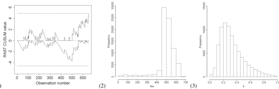
Fig. 1. (1) Risk-adjusted survival time CUSUM chart (h= 4.88) and obtained posterior distributions of (2) timeτ and (3) magnitudekof a decrease of sizek= 0.25inλ(mean survival time) whereλ0= 42133.6andτ= 500.
observations, and “Posterior” is the state of knowledge about the quantity after data are observed, which also is in the form of a probability distribution.
As discussed in Section I, in RAST CUSUM procedures, we let the survival function vary over patients and we control the observed survival time, which may be right censored, against the corresponding predicted survival function ob-tained through the survival time model. In this setting, a process is in the in-control state when observations can be statistically expressed by the underlying survival time model, taking into account their individual covariates. The RAST CUSUM signals when observations tend to violate the underlying model.
To model a change point in the presence of covariates, consider a process that results a survival time of ti, i =
1, ..., T, that is initially in-control. The observations can be explained by a survival function S(ti, ui)), where the
underlying distribution (f(.))is a Weibull distribution with (α0, λ0), and ui is a vectors of covariates. At an unknown
point in time, τ, the Weibull scale parameter changes from its in-control state ofλ0 toλ1,λ1=k×λ0,0< k <1. The right censored survival time step change model can thus be parameterized using survival function as follows:
S(ti, ui) =
exp h
−tiexp(β0Tui)
λ0
α0i
if i= 1,2, ..., τ
exph−tiexp(β0Tui)
λ1
α0i
if i=τ+ 1, ..., T
(4)
whereβ0 is the vector of covariate coefficients.
If desired, an overall estimation of change size in odds of mortality equivalent to a specific shift in the MST orλcan be obtained through simulation and averaging over different values of covariate,ui.
Relating this to Equation (3), the likelihood that underlies the observations is obtained throughf(.)δS(.)1−δ; see Sego
et al. [9]. The time and the magnitude of a drop in the MST are the unknown parameters of interest; and the posterior distributions of these parameters will be investigated in the change point analysis.
Assume that the process ti is monitored by a control
chart that signals at time T. We assign a truncated normal distribution (µ, σ)I(.) for k as prior distribution where all parameters are set study-specific. For a decrease inkwhich is detected by the upper RAST CUSUM, exceeding the upper threshold h, we set N(µ = 0.255, σ = 0.6)I(0.01,0.99).
This setting leads to relatively an informed prior for the magnitude of the fall.
Mean of the prior was set corresponds to the shift that the chart was calibrated to detect, see Section IV. The prior let to be sensitive in detection of low to nearly large falls in
k. Note that other distributions such as uniform and Gamma might also be of interest fork since it is always a positive value; see Gelman et al. [17] for more details on selection of prior distributions.
We place a uniform distribution on the range of (1,T−1) as prior for τ where T is set to the time of the signal of control charts. See the Appendix for the step change model code in WinBUGS.
IV. EVALUATION
We used Monte Carlo simulation to study the performance of the constructed BHM in step change detection following a signal from a RAST CUSUM control chart when a fall in mean survival time is simulated to occur at τ = 500. However, to extend to the results that would be obtained in practice, we considered the same cardiac surgery dataset that were used by Steiner et al. [2] and then Sego et al. [9] to construct risk-adjusted control charts for Bernoulli and time-to event variables, respectively. It was reported that this dataset contains 6449 operations information that were performed between 1992-1998 at a single surgical center in U.K. The Parsonnet score [22] was recorded to quantify the patient’s risk prior to the cardiac surgery. A follow-up period of 30 days after the surgery was set as the censoring time. A Weibull AFT model with parameters of
ˆ
α0 = 0.4909,λˆ0= 42133.6 andβˆ0 = 0.1307 was reported by Sego et al. [9] when the first two years of the data set were used as training data to fit the model and construct in-control state of the process and RAST CUSWUM. They also found that the recorded Parsonnet scores of the training data can be well approximated by an exponential distribution with a mean of 8.9.
To generate right censored survival time observations of a process in the in-control state ti, i = 1, ..., τ,
we first randomly generated the Parsonnet score, ui,
i = 1, ..., τ, from an exponential distribution with a mean of 8.9 and then drew associated survival time,
xi, i = 1, ..., τ, from the Weibull AFT model with
IAENG International Journal of Applied Mathematics, 41:4, IJAM_41_4_13
α0 = 0.4909, λ0 = 42133.6, and β0 = 0.1307. Finally, ti
andδiwere obtained considering a censoring time ofc= 30
through Equation 1. Plotting the obtained observations when the associated covariates are considered results a RAST CUSUM chart that is in-control. To generate the drops in λ0, or MST, we then induced changes of sizes k = {0.05,0.066,0.1,0.143,0.20,0.25,0.33,0.50,0.66,0.75} and generated observations until the control charts signalled. These changes led to different change sizes in in-control estimated survival probability over days for a patient with ui as well as survival curves between patients with
different Parsonnet scores. Note that other distributions such as uniform distributions with proper parameters or even sampling randomly from the baseline Parsonnet scores can be applied to generate covariates directly.
To construct RAST CUSUM, we applied the procedures discussed in Section II. We calibrated RAST CUSUM to detect a decrease in the MST that correspond to a doubling of the odds ratio within the follow-up period and has an in-control average run length (ARLˆ 0) of approximately 10000 observations. As mentioned in Section II, for the Weibull AFT model the corresponding odds ratio formula, discussed by Segoet al. [9], is not reduced to a close form ofλ0 and
ρsince the covariate term is not simplified. in
OR= Oi1
Oi0
, and Oi=
1−S(c|ui)
S(c|ui)
(5)
where S(c |ui) is the probability of survival at the end of
follow-up period,c.
Therefore we used Monte Carlo simulation to estimate corresponding ρ. To do so, we set ρ such over 100,000 replications of generating Parsonet scores from the fitted exponential distribution with a mean of 8.9 and calculating the odds in Equation 5, the desired odds ratio of sizeOR= 2 was obtained. A decrease ofρˆ= 0.255in the MST was found correspond to the desired jump in odds ratio.
We also used Monte Carlo simulation to determine the decision interval, h. However other approaches may be of interest; see Steiner et al. [2] and Sego et al. [9]. This setting led to a decision interval ofh= 4.88. The associated CUSUM scores were also obtained through Equation (2) considering the generatedti, δi andui.
The step change and control charts were simulated in the R package (http://www.r-project.org). To obtain posterior distributions of the time and the magnitude of the changes we used the R2WinBUGS interface [23] to generate 100,000 samples through MCMC iterations in WinBUGS [24] for all change point scenarios with the first 20000 samples ignored as burn-in. We then analyzed the results using the CODA package in R [25]. See the Appendix for the step change model code in WinBUGS.
V. PERFORMANCEANALYSIS
To demonstrate the achievable results of Bayesian change point detection in risk-adjusted control charts, we induced a drop of size = 0.25 at time τ = 500 in an in-control process with an overall survival time of λ0 = 42133.6. RAST CUSUM detected the drop and sinalled at the 651st observation, corresponding to a delay of 151 observations as shown in Figure 1-1. The posterior distributions of time and magnitude of the change were then obtained using
TABLE I
POSTERIOR ESTIMATES(MODE,SD.)OF STEP CHANGE POINT MODEL PARAMETERS(τANDk)FOLLOWING SIGNALS(RL)FROMRAST
CUSUM (h= 4.88)WHEREλ0= 42133.6ANDτ= 500.
k RL τˆ σˆˆτ ˆk σˆkˆ
0.25 651 499.8 96.0 0.226 0.18 0.33 722 494.8 160.6 0.27 0.19
MCMC discussed in Section IV. The distribution of the time of the change, τ, concentrates on the 500th observation,
approximately, as seen in Figure 1-2. The posterior for the magnitude of the change, k, also reasonably identified the exact change size as it highly concentrates on values of around 0.25 shown in Figure 1-3.
This investigation was replicated using a smaller shift of size k = 0.33 in λ. Table I summarizes the posterior estimates for both change sizes. If the posterior was asym-metric and skewed, the mode of the posterior was used as an estimator for the change point model parameters (τ and
k).
The RAST CUSUM signalled after 222 observations when the mean survival time became a third whereas the posterior distribution reported a drop at the 491st observation. This result implies that although the obtained posterior estimates underestimated the change point, they still performed signif-icantly better than the RAST CUSUM charts.
Bayesian estimates of the magnitude of the change tend to be relatively accurate following signals of the control chart, see Figure 1-3 and Table I. The slight bias, here underestimation, observed in the figures must be considered in the context of their corresponding standard deviations.
Comparison of estimates obtained across change sizes reveals that although a shorter run of observations from the out-of control state of the process is used when a larger shift size occurred, less dispersed posteriors are obtained, particularly for posteriors of time.
Applying the Bayesian framework enables us to construct probability based intervals around estimated parameters. A credible interval (CI) is a posterior probability based interval which involves those values of highest probability in the pos-terior density of the parameter of interest. Table II presents 50% and 80% credible intervals for the estimated time and the magnitude of changes in λ0 for the RAST CUSUM chart. As expected, the CIs are affected by the dispersion and higher order behaviour of the posterior distributions. Under the same probability of 0.5, the CI for the time of the change of size k= 0.25 covers 63 obsrevations around the 500th observation whereas it increases and reaches to
161 observations for k = 0.33 due to the larger standard deviation, see Table I. This investigation can be extended to other shift sizes for the time estimates. As shown in Table I and discussed above, the magnitude of the changes are
TABLE II
CREDIBLE INTERVALS FOR STEP CHANGE POINT MODEL PARAMETERS
(τANDk)FOLLOWING SIGNALS(RL)FROMRAST CUSUM (h= 4.88)
WHEREλ0= 42133.6ANDτ= 500.
k CI 50% CI 80%
ˆ
τ ˆk ˆτ ˆk
0.25 (488, 551) (0.14, 0.33) (453, 581) (0.09, 0.48) 0.33 (487, 648) (0.15, 0.40) (359, 709) (0.09, 0.57)
IAENG International Journal of Applied Mathematics, 41:4, IJAM_41_4_13
TABLE III
PROBABILITY OF THE OCCURRENCE OF THE CHANGE POINT IN THE LAST{25, 50, 100, 200, 300, 400, 500}OBSERVATIONS PRIOR TO SIGNALLING FORRAST CUSUM (h= 4.88)WHEREλ0= 42133.6ANDτ= 500.
k 25 50 100 200 300 400 500
0.25 0.03 0.07 0.20 0.89 0.94 0.96 0.97
0.33 0.01 0.05 0.20 0.59 0.77 0.82 0.90
also estimated reasonably well and Table II shows that in all cases the real sizes of changes are contained in the respective posterior 50% and 80% CIs.
Having a distribution for the time of the change enables us to make other probabilistic inferences. As an example, Table III shows the probability of the occurrence of the change point in the last {25, 50, 100, 200, 300, 400, 500} observations prior to signalling in the control charts. For a step change of sizek= 0.33in the mean survival time, since the RAST CUSUM signals late (see Table I), it is unlikely that the change point occurred in the last 100 observations. A considerable growth in the probability is seen when the next 200 observations are included, reaching to 0.77, whereas for a larger drop of size k = 0.25, it is more certain that the change point has occured in the last 200 observations with a probability of 0.89.
The above studies were based on a single sample drawn from the underlying distribution. To investigate the behavior of the Bayesian estimator over different sample datasets, for different reduction in λ0, we replicated the simulation method explained in Section IV 100 times.
Table IV shows the average of the estimated parameters obtained from the replicated datasets where there exists a drop in λ0 of sizek.
As seen, the RAST CUSUM control chart tends to detect larger shifts in the MST with less delays. For a large drop, a
kof size 0.143 and less, the chart signals with a delay of at most 95 observations. This delay increases over moderates reductions inλ0, reaching to 279 observations fork= 0.33. However, the chart is failed in detection of small drops since signals with a long delay of more than 639 observations obtained when the MST halved, k= 0.50.
For large drops in the MST, akof size 0.143 and less, the average values of the modes, Eˆ(ˆτ), tends to underestimate the time of the change since it reports at best the 490th observation fork= 0.066. However, the Bayesian estimator still outperforms the chart signal with a less bias over large reductions. This superiority persists for moderate shifts in the MST, where a less bias is still associated with the Bayesian estimates of the time,τ, at best three observations obtained for k = 0.20. Although the RAST CUSUM chart was designed to detect a moderate drop of 0.255 in the MST, it is outperformed by the posterior mode that detects the change point with a delay of 27 observations.
Table IV shows that the bias of the Bayesian estimator, ˆ
E(ˆτ), did not exceed 55 observations over moderate re-ductions. This bias increased when the MST halved, reach-ing to 162 observations, yet significantly outperformed the chart’s signal. For smaller reductions,k = (0.66,0.75), the posterior modes significantly overestimate the change point since the RAST CUSUM signals very late. The variation of the Bayesian estimates for time tends to reduce when the magnitude of shift in the MST increases. The mean of the standard deviation of the posterior estimates of time,Eˆ(στˆ), also decreases when shift sizes increase.
Table IV indicates that the average of the Bayesian estima-tor of the magnitude of the change,Eˆ(ˆδ), identifies change sizes with some biases. This estimator tends to overestimate and underestimate the sizes where there exist large drops and moderate to small drops, respectively. Having said that, Bayesian estimates of the magnitude of the change must be studied in conjunction with their corresponding standard deviations. In this manner, analysis of credible intervals is
TABLE IV
AVERAGE OF POSTERIOR ESTIMATES(MODE,SD.)OF STEP CHANGE POINT MODEL PARAMETERS(τANDk)FOR A CHANGE IN THE MEAN SURVIVAL TIME FOLLOWING SIGNALS(RL)FROMRAST CUSUM (h= 4.88)WHEREλ0= 42133.6ANDτ= 500. STANDARD DEVIATIONS ARE SHOWN IN
PARENTHESES.
k Eˆ(RL) Change point Change size ˆ
E(ˆτ) Eˆ(ˆστˆ) Eˆ(ˆk) Eˆ(ˆσˆk)
0.05 542.4 486.0 91.2 0.077 0.173
(16.2) (57.3) (34.7) (0.086) (0.022)
0.066 554.8 490.5 92.9 0.083 0.177
(26.6) (62.5) (36.7) (0.075) (0.025)
0.10 568.3 485.7 99.4 0.127 0.183
(39.7) (70.9) (33.9) (0.094) (0.017)
0.143 594.2 487.3 110.9 0.154 0.185
(49.2) (72.5) (34.5) (0.090) (0.016)
0.20 624.7 503.7 119.5 0.182 0.183
(71.3) (87.1) (36.6) (0.103) (0.018)
0.25 692.3 527.3 132.9 0.211 0.183
(150.4) (146.2) (53.4) (0.111) (0.018)
0.33 (187.7)779.6 (162.3)554.3 (58.9)153.9 (0.118)0.25 (0.023)0.176
0.50 (605.0)1139.0 (287.7)661.8 (173.0)258.9 (0.16)0.43 (0.028)0.178
0.66 (2169.8)2469.4 (783.2)1270.3 (456.6)562.1 (0.22)0.51 (0.047)0.183
0.75 2773.4 1748.0 697.9 0.53 0.195
(2195.4) (1304.4) (720.8) (0.25) (0.047)
IAENG International Journal of Applied Mathematics, 41:4, IJAM_41_4_13
effective.
VI. CONCLUSION
Quality improvement programs and monitoring of medical process outcomes are now being widely implemented in the health context to achieve stability in outcomes through detection of shifts and investigation of potential causes. Obtaining accurate information about the time when a change occurred in the process has been recently considered within industrial and business quality control applications. Indeed, knowing the change point enhances efficiency of root cause analysis efforts by restricting the search to a tighter window of observations and related variables.
In this paper, using a Bayesian framework, we modeled change point detection in time-to-event data for a clinical process with dichotomous outcomes, death and survival, where patient mix was present. We considered a drop in the mean of survival time of an in-control process. We con-structed Bayesian hierarchical models and derived posterior distributions for change point estimates using MCMC. The performance of the Bayesian estimators were investigated through simulation when they were used in conjunction with risk-adjusted survival time CUSUM control charts monitor-ing right censored survival time of patients who underwent cardiac surgery procedures within a follow-up period of 30 days where the severity of risk factors prior to the surgery was evaluated by the Parsonnet score. The results showed that the Bayesian estimates significantly outperform the RAST CUSUM control charts in change detection over different magnitude of drops in the mean survival time.
Apart from accuracy and precision criteria used for the comparison study, the posterior distributions for the time and the magnitude of a change enable us to construct probabilistic intervals around estimates and probabilistic inferences about the location of the change point. This is a significant ad-vantage of the proposed Bayesian approach. Furthermore, flexibility of Bayesian hierarchical models, ease of extension to more complicated change scenarios such as linear and non-linear trends in survival time, relief of analytic calculation of likelihood function, particularly for non-tractable likelihood functions and ease of coding with available packages should be considered as additional benefits of the proposed Bayesian change point model for monitoring purposes.
The investigation conducted in this study was based on a specific in-control rate of mortality observed in the pilot hos-pital. Although it is expected that superiority of the proposed Bayesian estimator persists over other processes in which the in-control rate and the distribution of baseline risk may differ, the results obtained for estimators and control charts over various change scenarios motivates replication of the study using other patient mix profiles. Moreover modification of change point model elements such as replacing priors with more informative alternatives may be of interest.
The two-step approach to change-point identification de-scribed in this paper has the advantage of building on control charts that may be already in place in practice (as in the pilot hospital). An alternative may be to retain the two-step approach but to use a Bayesian framework in both stages. There is now a substantial literature on Bayesian formulation of control charts and extensions such as monitoring processes
with varying parameters [26], over-dispersed data [27], start-up and short runs [28], [29]. A further alternative is to consider a fully Bayesian, one-step approach, in which both the monitoring of the in-control process and the retrospective or prospective identification of changes is undertaken in the one analysis. This is the subject of further research.
APPENDIXA
CHANGE POINT MODEL CODE INWINBUGS
model{
for(i in 1 : RLcusum) {
y[i]∼dweib(alpha0, gamma[i])I(yc[i],) gamma[i] = pow(exp(beta0 * riskscore[i])/
(lambda0+step(i-tau) * lambda0 * (k-1)), alpha) }
RL=RLcusum-1
k∼dnorm(0.255, 2.77)I(0.01, 0.99) tau∼dunif(1, RL)}
REFERENCES
[1] Montgomery D.C.,Introduction to Statistical Quality Control(Sixth ed.): Wiley, 2008.
[2] Steiner, S.H., Cook, R.J., Farewell, V.T., & Treasure, T., “Monitoring surgical performance using risk-adjusted cumulative sum charts”, Biostatistics, V1, N4, pp. 441-452, 2000.
[3] Cook, D., “The Development of Risk Adjusted Control Charts and Machine learning Models to monitor the Mortality of Intensive Care Unit Patients”,Ph.D. Thesis; University of Queensland, 2004. [4] Grigg, O.V. & Spiegelhalter, D.J., “A Simple Risk-Adjusted
Exponen-tially Weighted Moving Average”,Journal of the American Statistical Association, V102, N477, pp. 140-152, 2007.
[5] Grigg, O. V., & Farewell, V. T., “An overview of risk-adjusted charts”, Journal of the Royal Statistical Society: Series A (Statistics in Society), V167, N3, pp. 523-539, 2004.
[6] Grigg, O. V., & Spiegelhalter D. J., “Discussion”,Journal of Quality Technology, V38, N2, pp. 124-136, 2006.
[7] Cook, D. A., Duke, G., Hart, G. K., Pilcher, D., Mullany, D., “Review of the application of risk-adjusted charts to analyse mortality outcomes in critical Care”,Critical Care Resuscitation, V10, N3, pp. 239-251, 2008.
[8] Biswas, P. & Kalbfliesch, J.D., “A risk-adjusted CUSUM in continuous time based on the Cox model,”Statistics in Medicine, V 27, N17, pp. 3382-3406, 2008.
[9] Sego, L.H., Reynolds, Jr.M.R., Woodall, W.H., “Risk adjusted monitor-ing of survival times”,Statistics in Medicine, V28, N9, pp. 1386-1401, 2009.
[10] Steiner, S.H. & Jones, M., “Risk-adjusted survival time monitoring with an updating exponentially weighted moving average (EWMA) control chart”,Statistics in Medicine, V29, N4, pp. 444-454, 2010. [11] Assareh, H., Smith, I., Mengersen, K., “Bayesian change point
detec-tion in monitoring cardiac surgery outcomes”,Quality Management in health Care, V20, N3, pp. 207-222, 2011.
[12] Samuel, T. & Pignatjello, J., “Identifying the time of a step change in the process fraction nonconforming”,Quality Engineering, V13 , N3 , pp. 357-365, 2001.
[13] Perry, M. & Pignatiello, J., “Estimating the change point of the process fraction nonconforming in SPC applications”, International Journal of Reliability, Quality and Safety Engineering, V12, N2, pp. 95-110, 2005.
[14] Box, G. & Cox, D., “An analysis of transformations”,Journal of the Royal Statistical Society. Series B (Methodological), V26, N2, pp. 211-252, 1964.
[15] Noorossana, R., Saghaei, A., Paynabar, K. & Abdi, S., “Identifying the period of a step change in high-yield processes”, Quality and Reliability Engineering International, V25, N7, pp. 875-883, 2009. [16] Xie, M., Goh, T. & Kuralmani, V., Statistical Models and Control
Charts for High-Quality Processes: Kluwer Academic Publishers, 2002.
[17] Gelman, A., Carlin, J., Stern, H. & Rubin, D.,Bayesian Data Analysis: Chapman&Hall/CRC, 2004.
IAENG International Journal of Applied Mathematics, 41:4, IJAM_41_4_13
[18] Assareh, H., Smith, I. & Mengersen, K., “Identifying the time of a linear trend disturbance in odds ratio of clinical outcomes”,Lecture Notes in Engineering and Computer Science: Proceedings of The World Congress on Engineering 2011, V1, WCE 2011, 6-8 July, London, U.K., pp. 365-370, 2011.
[19] Assareh, H.& Mengersen, K., “Detection of the time of a step change in monitoring survival time”,Lecture Notes in Engineering and Com-puter Science: Proceedings of The World Congress on Engineering 2011, V1, WCE 2011, 6-8 July, London, U.K., pp. 314-319, 2011. [20] Klein, J.P. & Moeschberger, M.L.,Survival Analysis: Techniques for
Censored and Truncated Data.Springer: New York, 1997.
[21] Sego, L.H., “Applications of control charts in medicine and epi-demiology”,PhD Thesis, United States-Virginia, Virginia Polytechnic Institute and State University, 2006.
[22] Parsonnet, V., Dean, D., Bernstein, A.D., “A method of uniform stratification of risk for evaluating the results of surgery in acquired adult heart disease”,CirculationV79, 6 Pt 2, pp. I3-12, 1989. [23] Sturtz, S., Ligges, U., & Gelman, A., “R2WinBUGS: A package for
running WinBUGS from R”,Journal of Statistical Software, V12, N3, pp. 1-16, 2005.
[24] Spielgelhalter, D., Thomas, A. & Best, N., WinBUGS version 1.4. Bayesian inference using Gibbs sampling.Manual. MRC Biostatistics Unit. Institute for Public Health, Cambridge, United Kingdom, 2003. [25] Plummer, M., Best, N., Cowles, K. & Vines, K., Output analysis and diagnostics for MCMC. R package version 0.10-3, URL http://cran.r-project.org, 2005.
[26] Feltz, C. J. & Shiau, J.-J. H., “Statistical process monitoring using an empirical Bayes multivariate process control chart”,Quality and Reliability Engineering International, V17, N2, pp. 119-124, 2001. [27] Bayarri, M. J. & Garcia-Donato, G., “A Bayesian Sequential Look at
u-Control Charts”,Technometrics, V47, N2, pp. 142-151, 2005. [28] Tsiamyrtzis, P. & Hawkins, D. M., “A Bayesian Scheme to Detect
Changes in the Mean of a Short-Run Process”,Technometrics, V47 ,N4, 446-456, 2005.
[29] Tsiamyrtzis, P. & Hawkins, D. M., “A Bayesian EWMA method to detect jumps at the start-up phase of a process”,Quality and Reliability Engineering International, V24 ,N6, 721-735, 2008.