Preconditioned Parallel Multisplitting USAOR Methods for Hmatrices Linear Systems

(1)

Preconditioned Parallel Multisplitting USAOR

Methods for

H

−

matrices Linear Systems

Xuezhong Wang, Zuowei Wang

Abstract—In this paper, three preconditioned parallel mul-tisplitting methods are established for solving the large sparse linear systems, including local preconditioned parallel mul-tisplitting relaxation method, global preconditioned parallel multisplitting relaxation method and global preconditioned nonstationary parallel multisplitting relaxation method. The convergence and comparison results of the methods associat-ed with USAOR multisplitting are given when the coefficient matrices of the linear systems are H-matrices. We prove three preconditioned parallel multisplitting USAOR method are better than parallel multisplitting USAOR methods for M-matrices linear systems. Finally, numerical examples are given to illustrate the methods are valid.

Index Terms—Preconditioned, Relaxation parallel multi-splitting method, Convergence, USAOR,H-matrix.

I. INTRODUCTION

F

OR the linear system

A x=b, (1)

where A is an n× n square matrix, and x and b are

n-dimensional vectors. The basic iterative method for solving equation (1) is

M xk+1=N xk+b, k=0, 1,···, (2) whereA=M−N andM is nonsingular. Thus (2) can be written as

xk+1=T xk+c, k=0, 1,···, (3) whereT=M−1N,c=M−1b.

The original systems (1) can be transformed into the preconditioned form

P A x=P b. (4)

Then, we can define the basic iterative scheme:

Mpxk+1=Npxk+P b, k=0, 1,···, (5) whereP A=Mp−Np andMp is nonsingular. Thus (5) can also be written as

xk+1=T xk+c, k=0, 1,···, whereT=M−1

p Np, c=Mp−1P b.

Without loss of generality, we assume thatA has unit diagonal elements. In the literature, various authors have suggested different models of(I+S)-type preconditioner

[1-7, 24-28] for linear systems (1). These precondition-ers have effectiveness and low construction cost. For

Manuscript received September 08, 2013; revised January 27, 2014. X. Z. Wang is with School of Mathematics and Statistic-s, Hexi University, Zhangye, Gansu, 734000, P. R. C., e-mail: [email protected].

Z. W. Wang is with College of Foreign Language and Litera-ture, Hexi University, Zhangye, Gansu, 734000, P. R. C., e-mail: [email protected].

example, in this paper, we consider the preconditioner of(I+S)-type with the following form

P=I+S_α−S_β, (6)

where

I+S_α=          

1 α1r

1 α2s

...

αi u ...

...

αn t 1

         

,

and

S_β=          

0 β1a1r

0 β2a2s

...

βiai u ...

...

βnan t 0

         

.

O’Leary and White [8] invented the matrix multi-splitting method in 1985 for parallely solving the large sparse linear systems on the multiprocessor systems and it was further studied by many authors [9-19]. For example, Neumann and Plemmons[12]developed some more refined convergence results for one of the cases considered in[8]. Elsner[13]established the comparison theorems about the asymptotic convergence rate of this case. Frommer and Mayer[14] discussed the successive overrelaxation (SOR) method in the sense of multisplit-ting. White[15]studied the convergence properties of the above matrix multisplitting methods for the symmetric positive definite matrix class. Zhang, Huang, et al. [9] presented local relaxed parallel multisplitting method and global relaxed parallel multisplitting method forH -matrices, and so on.

A collection of triples (Mk,Nk,Ek), k = 1, 2, . . . ,α, is called a multisplitting ofA. IfA=Mk−Nk is a splitting of

A for k=1, 2, . . . ,α, and Ek’s, called weighting matrices, are nonnegative diagonal matrices such that ∑α

k=1

e_{i i}(k)=1. The multisplitting method associated with this multisplit-ting for solving the linear system (1) is as follows.

Suppose that we have a multiprocessor with α pro-cessors connected to a host processor, that is, the same number of processors as splittings, and all the processors have the last update vector xk_{, then the} _k_{th processor} only computes those entries of the vector

M_k−1Nkxk+M_k−1b,

IAENG International Journal of Applied Mathematics, 44:1, IJAM_44_1_06

(2)

which correspond to the diagonal entries E_{i i}(k) of the matrixEk. The processor then scales these entries so as to be able to deliver the vector

EK(Mk−1Nkxk+Mk−1b),

to the host processor, performing the parallel multisplit-ting scheme

xm+1= α ∑

k=1

EkMk−1Nkxm+

α ∑

k=1

EkMk−1b =H xm+G b,m=0, 1, 2, . . . .

Under certain conditions, we establish local precon-ditioned parallel multisplitting relaxation method, global preconditioned parallel multisplitting relaxation method and global preconditioned nonstationary parallel multi-splitting relaxation method for solving the large sparse linear systems and study the convergence of our methods associated with USAOR multisplitting when the coeffi-cient matrices of the linear systems are H-matrices.

II. ESTABLISHMENTS OF THE METHODS

Let A=I−Lk−Uk,k=1, 2, . . . ,α, where I is a identity matrix, Lk, k = 1, 2, . . . ,α, are strictly lower triangular matrices, andUk,k=1, 2, . . . ,α, are general matrices, re-spectively, then parallel multisplitting relaxation USAOR methods are defined[9]as follows.

Algorithm 2.1. (local parallel multisplitting relaxation

method)

Given the initial vector. Form=0, 1, 2, . . . repeat (I) and (II), until convergence.

(I) For k=1, 2, . . . ,α, (parallel) solving yk:

Mkyk=Nkxm+b. (II) Computing

xm+1= α ∑

k=1 Ekyk.

Algorithm 2.1 associated with LUSAOR method can be written as

xm+1=HLU S AO Rxm+GLU S AO Rb, m=0, 1,···, where

HLU S AO R =

α ∑

k=1

EkUω2r2(k)Lω1r1(k),

U_ω₂r2(k) = (I−r2Uk)

−1_[(₁₋_ω 2)I

+(ω2−r2)Uk +ω2Lk],

L_ω₁r1(k) = (I−r1Lk)

−1_[(₁₋_ω

1)I+ (ω1−r1)Lk +ω1Uk],

GLU S AO R =

α ∑

k=1

Ek(I−r2Uk)−1[(ω1+ω2 −ω1ω2)I+ω2(ω1−r1)Lk +ω1(ω2−r2)Uk](I−r1Lk)−1.

By using a suitable positive relaxation parameter β, global parallel multisplitting relaxation USAOR method will be established in the following, which is based on Algorithm 2.1.

Algorithm 2.2.(global parallel multisplitting relaxation

method)

(I) Fork=1, 2, . . . ,α, (parallel) solving yk:

Mkyk=Nkxm+b.

(II) Computing

xm+1=β

α ∑

k=1

Ekyk+ (1−β)xm.

Algorithm 2.2 associated with GUSAOR method can be written as

xm+1=HG U S AO Rxm+βGLU S AO Rb,m=0, 1,···,

whereHG BU S AO R=βHL BU S AO R+ (1−β)I.

In the standard multisplitting method, each local ap-proximation is updated exactly once by using the same previous iterate xm_{. On the other hand, it is possible} to update the local approximations more than once, by using different iterates computed earlier. In this case, we call this method a nonstationary multisplitting method

[17,18,19]. The main idea of the nonstationary method is that at the mth iteration each processork solves the systemq(m,k)times, using each time the new calculated vector to update the right-hand side, i.e., we have the following algorithm:

Algorithm 2.3. (global nonstationary parallel

multi-splitting relaxation method)

(I) Fori=1, 2, . . . ,q(m,k), (parallel) solving y_k(i):

Mkyk(i)=Nkyk(i−1)+b. (II) Computing

xm+1=β α ∑

k=1 Eky

q(m,k)

k + (1−β)x m_.

Algorithm 2.3 associated with GNUSAOR method can be written as

xm+1=HG N U S AO Rxm+βGG N U S AO Rb, m=0, 1,···,

where

HG N U S AO R = β

α ∑

k=1Ek(PωrQξη)

q(m,k)_{+ (}₁₋_β₎_I

P_ωr = (I−rkUk)−1[(1−ωk)I+ (ωk−rk)Uk +ωkLk] =Wr−1Rωr,

Q_ξη = (I−ηkLk)−1[(1−ξk)I+ (ξk−ηk)Lk +ξkUk] =V_η−1Fξη,

GG N U S AO R = β

α ∑

k=1 Ek[

q(m∑,k)−1

i=1 ( WrVη)−1

(F_ξηR_ωr)i](WrVη)−1ωkξk.

It follows that whenq(m,k) =1, ωk=ω2,rk=r2,ξk=

ω1 and ηk=r1 for 1<k< α,m=0, 1, 2...., Algorithm 2.3

reduces to Algorithm 2.2.

Let ˜A=P A=D˜−L˜k−U˜k, k=1, 2, . . . ,α, where ˜D is a diagonal matrix, ˜Lk,k=1, 2, . . . ,α, are strictly lower trian-gular matrices, and ˜Uk,k=1, 2, . . . ,α, are general matri-ces, respectively. Then Algorithm 2.1 associated with local

IAENG International Journal of Applied Mathematics, 44:1, IJAM_44_1_06

(3)

preconditioned parallel multisplitting relaxation method (LPUSAOR) can be written as

xm+1=H˜L P U S AO Rxm+G˜L P U S AO Rb, m=0, 1,···, where

˜

HL P U S AO R =

α ∑

k=1Ek

˜

U_ω₂r2(k)L˜ω1r1(k),

˜

U_ω₂r2(k) = (D˜−r2U˜k)

−1_[(₁₋_ω 2)D˜

+(ω2−r2)U˜k+ω2L˜k], ˜

L_ω₁r1(k) = (D˜−r1L˜k)

−1_[(₁₋_ω 1)D˜

+(ω1−r1)L˜k+ω1U˜k], ˜

GL P U S AO R =

α ∑

k=1

Ek(D˜−r2U˜k)−1[(ω1+ω2 −ω1ω2)D˜+ω2(ω1−r1)L˜k

+ω1(ω2−r2)U˜k](D˜−r1L˜k)−1. Algorithm 2.2 associated with global preconditioned parallel multisplitting relaxation method (GPUSAOR) method can be written as

xm+1=H˜G P U S AO Rxm+βG˜L P U S AO Rb, m=0, 1,···, (7) where ˜HG P U S AO R=βH˜L P U S AO R+ (1−β)I.

Algorithm 2.3 associated with global preconditioned nonstationary parallel multisplitting relaxation method (GPNUSAOR) can be written as

xm+1=H˜G P N U S AO Rxm+βG˜G P N U S AO Rb, m=0, 1,···, where

˜

HG P N U S AO R = β

α ∑

k=1

Ek(P˜ωrQ˜ξη)q(m,k)

+(1−β)I

˜

P_ωr = (D˜−rkU˜k)−1[(1−ωk)D˜

+(ωk−rk)U˜k+ωkL˜k] =W˜r−1R˜ωr, ˜

Q_ξη = (D˜−ηkL˜k)−1[(1−ξk)D˜+ (ξk−ηk)L˜k+ξkU˜k] =V˜_η−1F˜ξη, ˜

GG P N U S AO R = β

α ∑

k=1 Ek[

q(m∑,k)−1

i=1 (

˜

W_ωV˜_η)−1

(_F˜_ξη_R˜_ω_r₎i_](_W_˜

ωV˜η)−1ωkξk.

Obviously, when q(m,k) =1, ωk =ω2, rk =r2, ξk =

ω1 and ηk =r1 for 1<k< α, m=0, 1, 2...., GPNUSAOR method reduces to GPUSAOR method.

III. PRELIMINARIES

We shall use the following notations and lemmas. A matrixA is called nonnegative (positive) if each entry of

Ais nonnegative (positive), respectively. We denote them by A≥0 (A>0). Similarly, for n-dimensional vector x, by identifying them withn×1 matrix, we can also define

x≥0 (x>0). A matrixA= (ai j)is called aZ-matrix if for anyi̸=j,ai j≤0. AZ-matrix is a nonsingularM-matrix if A is nonsingular and if A−1_≥_{0. We call} _〈A〉_{= (}_a_¯

i j) its comparison matrix, if(a¯i j) =|ai j|fori=j, if(a¯i j) =−|ai j| fori̸=j. If〈A〉is a nonsingularM-matrix, thenAis called anH-matrix.A=M−N is said to be a splitting ofAifM

is nonsingular,A=M−N is said to be regular ifM−1_≥₀

and N ≥0, and weak regular if M−1_≥_{0 and} _M−1_N _≥_0.

Additionally, we denote the spectral radius of Abyρ(A). It is well-known that if A≥0 and there exists a vector

x>0, such that A x< αx, thenρ(A)< α.

Some basic properties are given below, which will be used in the paper.

Lemma 3.1[21].Let A be a Z-matrix. Then the

follow-ing statements are equivalent: (a) A is an M-matrix.

(b) There is a positive vector x such thatA x>0. (c)A−1_≥_0.

(d) All principal submatrices of A are M-matrices. (e) All principal minors are positive.

Lemma 3.2 [20]. Let A=M−N be an M-splitting of

A, thenρ(M−1_N₎_<_{1 if and only if}_A _{is an M-matrix.}

Lemma 3.3 [20]. Let A and B be two n×n matrices

with 0≤B≤A, thenρ(B)≤ρ(A).

Lemma 3.4 [22]. If A is an H−matrix, then |A−1_{| ≤}

〈A〉−1_.

Lemma 3.5 [12].Suppose that A1=M1−N1 and A2=

M2−N2 are weak regular splitting of monotone matrices A1 and A2 respectively, such that M2−1≥M1−1. If there

exists a positive vector x such that 0≤A1x≤A2x, then

for the monotone norm associated withx,

∥M₂−1N2∥x≤∥M1−1N1∥x. (8) In particular, ifM−1

1 N1has a positive perron vector, then

ρ(M₂−1N2)≤ρ(M1−1N1). (9)

Moreover if x is a Perron vector of M−1

1 N1 and strictly

inequality holds in (8), then strictly inequality holds in (9).

Lemma 3.6 [9]. Let A be an H-matrix, and for k =

1, 2, . . . ,α,Lk be strictly lower triangular matrices. Define the matricesUk,k=1, 2, . . . ,α, such that A=D−Lk−Uk. Assume that〈A〉=|D| − |Lk| − |Uk|=|D| − |B|. If

0< ω1,ω2<

2

1+ρ, 0≤r1≤ω1, 0≤r2≤ω2,

then LUSAOR method converges for any initial vectorx0_,

whereρ=ρ(J) =ρ(|D|−1_|B_|₎_.

0< ω1,ω2<

2

1+ρ, 0≤r1≤ω1, 0≤r2≤ω2, 0< β < 2 1+θ,

then GUSAOR method converges for any initial vector

x0, whereρ=ρ(J) =ρ(|D|−1|B|) and

θ=m a x{|1−ω1|+ω1ρ,|1−ω2|+ω2ρ}.

0< ωk,ξk< 2

1+ρ, 0≤rk≤ωk, 0≤ηk≤ξk, 0< β < 2 1+θ′

then GUSAOR method converges for any initial vector

x0, whereρ=ρ(J) =ρ(|D|−1|B|) and

θ′₌_{m a x}_{|₁₋_ω

k|+ωkρ,|1−ξk|+ξkρ}.

LetA=M−N =F−Q are two splittings ofA. If we set

T=F−1Q M−1N.

IAENG International Journal of Applied Mathematics, 44:1, IJAM_44_1_06

(4)

Benzi and Szyld[23]have established the following result. Lemma 3.9 [23]. Let A−1_≥_{0. If the splitting} _A₌_M₋ N=F−Qare weak regular, thenρ(T)<1 and the unique splitting A=B−C induced by T is weak regular, where

B=F(M+P−A)−1_M _and _C₌_B₋_A_.

IV. CONVERGENCE

For Algorithms 1, 2 and 3, we give convergence theo-rems forH−matrices. For convenience, letti=2xm(〈−A(〉〈xA〉)ix)m, where x= (x1,x2,···,xn)T denotes a vector.

Theorem 4.1.LetAbe anH−matrix with unit diagonal

elements. Assume that there exists a positive vector

x= (x1,x2,···,xn)T, such that〈A〉x>0. If |αi m−βiai m| ≤

ti,i=1, 2,···,n, thenP A is an H−matrix.

Proof. Let (P A)i j = ai j + (αi m −βiai m)am j, i,j = 1, 2,···,n,m=r,s,···,t, and x= x1,x2,···,xn

T , then

(〈P A〉x)_i = 1+ αi m−βiai m

am i

xi

−ai m+ αi m−βiai mxm

− ∑

j̸=i,m

_a_{i j}₊ _α_{i m}₋_β_i_a_{i m}_a_{m j}_x_j

≥ xi−

_α_{i m}₋_β_iai m

_|am i|xi− |ai m|xm

−αi m−βiai m

_x_m₋ ∑

j̸=i,m

_a_{i j}_x_j

− ∑

j̸=i,m

_α_{i m}₋_β_i_a_{i m}_a_{m j}_x_j

¬ d.

Case 1.βiai m≤αi m≤βiai m+ti

d ≥ xi−(αi m−βiai m)|am i|xi− |ai m|xm

−(αi m−βiai m)xm−

∑

j̸=i,m

_a_{i j}_x_j

− ∑

j̸=i,m

(αi m−βiai m)

_a_{m j}_x_j

= xi− |ai m|xm−

∑

j̸=i,m

ai j

xj−(αi m−βiai m)|am i|xi

−(αi m−βiai m)xm−

∑

j̸=i,m

(αi m−βiai m)

_a_{m j}_x_j

= (〈A〉x)_i+ αi m−βiai m

(−xm−

∑

j̸=m

_a_{m j}_x_j₎

= (〈A〉x)i+ αi m−βiai m

(− ∑

j̸=m

_a_{m j}_x_j₊_x_m₋₂_x_m₎

= (〈A〉x)_i+ αi m−βiai m

[(〈A〉x)_m−2xm] > 0.

Case 2.βiai m−ti≤αi m≤βiai m

d ≥ xi+ αi m−βiai m

|am i|xi− |ai m|xm + αi m−βiai m

xm−

∑

j̸=i,m

_a_{i j}_x_j

+ ∑ j̸=i,m

αi m−βiai mam j

_x_j

(∑ j̸=m

_a_{m j}_x_j₋_x_m₊₂_x_m₎

[2xm−(〈A〉x)m]

> 0.

Therefore, 〈P A〉is an M-matrix, and P Ais an H-matrix. Together with Lemma 3.7, Lemma 3.8, Lemma 3.9 and Theorem 4.1, we can obtain the following results.

Theorem 4.2.LetAbe anH-matrix with unit diagonal

elements, and for k = 1, 2, . . . ,α, ˜Lk be strictly lower triangular matrices. Define the matrices ˜Uk,k=1, 2, . . . ,α, such that ˜A=P A=D˜−L˜k−U˜k. Assume that 〈A˜〉=|D˜| −

|_L˜_k_{| − |}_U˜_k_|₌_|_D˜_{| − |}_B|˜_{. If} _|_α_{i m}₋_β_i_a_{i m}_{| ≤}_t_i_,_i ₌_{1, 2,}_···_,_n_, and

0< ω1,ω2<

2

1+ρ˜, 0≤r1≤ω1, 0≤r2≤ω2, then LPUSAOR method converges for any initial vector

x0, where ˜ρ=ρ(J˜) =ρ(|D˜|−1|B˜|).

elements, and for k = 1, 2, . . . ,α, ˜Lk be strictly lower triangular matrices. Define the matrices ˜Uk,k=1, 2, . . . ,α, such that ˜A=P A=D˜−L˜k−U˜k. Assume that 〈A〉˜ =|D˜| −

0< ω1,ω2<

2

1+ρ˜, 0≤r1≤ω1, 0≤r2≤ω2, 0< β <

2 1+θ˜, then GPUSAOR method converges for any initial vector

x0_{, where ˜}_ρ₌_ρ₍_J_˜_{) =}_ρ₍_|_D_˜_|−1_|_B_˜_|₎ _and

˜

θ=m a x{|1−ω1|+ω1ρ˜,|1−ω2|+ω2ρ˜}.

elements, and for k = 1, 2, . . . ,α, ˜Lk be strictly lower triangular matrices. Define the matrices ˜Uk,k=1, 2, . . . ,α, such that ˜A=P A=D˜−L˜k−U˜k. Assume that 〈A〉˜ =|D˜| −

0< ωk,ξk< 2

1+ρ˜, 0≤rk≤ωk, 0≤ηk≤ξ2, 0< β < 2 1+θ˜′,

then GPNUSAOR method converges for any initial vector

x0_{, where ˜}_ρ₌_ρ₍_J_˜_{) =}_ρ₍_|_D_˜_|−1_|_B_˜_|₎ _and

˜

θ′=m a x{|1−ωk|+ωkρ˜,|1−ξk|+ξkρ˜}.

The proofs of Theorem 4.2, Theorem 4.3 and Theorem 4.4 are similar to Lemma 3.7, Lemma 3.8 and Lemma 3.9, respectively. So omitted.

V. COMPARISON RESULTS OF SPECTRAL RADIUS In what follows we will give some comparison re-sults on the spectral radius of preconditioned parallel multisplitting relaxation USAOR iteration matrices with preconditionerP. Let

〈A〉 = Mˆk−Nˆk=_ω1₁(|D| −r1|Lk|)

− 1

ω1[(1−ω1)I+ (ω1−r1)|Lk|+ω1|Uk|] = Mˆˆk−Nˆˆk=_ω1₂(|D| −r2|Uk|)

− 1

ω2[(1−ω2)I+ (ω2−r2)|Uk|+ω2|Lk|],

where

ˆ

Mk= 1

ω1

(|D| −r1|Lk|),

ˆ

Nk= 1

ω1

[(1−ω1)|D|+ (ω1−r1)|Lk|+ω1|Uk|],

and

ˆˆ

Mk= 1

ω2

(|D| −r2|Uk|),

ˆˆ

Nk= 1

ω2

[(1−ω2)|D|+ (ω2−r2)|Uk|+ω2|Lk|],

and then the iteration matrix of local parallel multisplit-ting relaxation USAOR method for〈A〉 is as follows

ˆ

HLU S AO R=

α ∑

k=1 EkMˆˆ

−1

k NˆˆkMˆk−1Nˆk.

IAENG International Journal of Applied Mathematics, 44:1, IJAM_44_1_06

(5)

Let

〈P A〉 = _M˜_k₋_N˜_k₌ 1 ω1(

˜

|D| −r1|L˜k|)−ω11[(1−ω1)

˜

|D|

+(ω1−r1)|L˜k|+ω1|U˜k|] = _M˜˜_k₋_N˜˜_k₌ 1

ω2(

˜

|D| −r2|U˜k|)−_ω1₂[(1−ω2)|D˜|

+(ω2−r2)|U˜k|+ω2|L˜k|], where

˜

Mk= 1

ω1

(_{|D| −}˜ _r_1|_L˜_k_|₎_,

˜

Nk= 1

ω1

[(1−ω1)|D˜|+ (ω1−r1)|L˜k|+ω1|U˜k|],

and

˜˜

Mk= 1

ω2

(_|D˜_{| −}_r_2|_U˜_k_|₎_,

˜˜

Nk= 1

ω2

[(1−ω2)|D˜|+ (ω2−r2)|U˜k|+ω2|L˜k|],

and then the iteration matrix of local preconditioned parallel multisplitting relaxation USAOR method for〈P A〉 is as follows

¨

HL P U S AO R=

α ∑

k=1 EkM˜˜

−1

k N˜˜kM˜k−1N˜k.

elements, and for k =1, 2, . . . ,α, ˜Lk and Lk be strictly lower triangular matrices. Define the matrices ˜Uk and

Uk, k =1, 2, . . . ,α, such that ˜A=P A =D˜−L˜k−U˜k and

A=I−Lk−Uk. Assume that 〈A〉˜ =〈P A〉=|D˜| − |L˜k| − |U˜k| and 〈A〉=I−|Lk|−|Uk|. If|αi m−βiai m| ≤ti,i=1, 2,···,n, and

0< ω1,ω2<1, 0≤r1≤ω1, 0≤r2≤ω2,

then ρ(H˜L P U S AO R)≤ρ(H¨L P U S AO R)≤ρ(HˆLU S AO R).

Proof. Since 〈A〉is a nonsingular M-matrix, it is easy

to show 〈A〉 =Mˆk −Nˆk =Mˆˆk −Nˆˆk are two weak reg-ular splittings. From Lemma 3.10, the unique splitting

〈A〉=_Bˆ_k₋_Cˆ_k _{induced by ˆˆ}_M−1

k NˆˆkMˆk−1Nˆk is weak regular s-plitting, where ˆBk=Mˆˆ(Mˆ+Mˆˆ−〈A〉)−1Mˆ and ˆCk=Bˆk−〈A〉, and then the iteration matrix of LUSAOR method for〈A〉

can be rewritten as ˆHLU S AO R=

α ∑

k=1Ek

ˆ

B_k−1Cˆk.

By Theorem 4.1,〈P A〉is a nonsingularM-matrix, and then 〈P A〉=M˜k −N˜k =M˜˜k−N˜˜k are two weak regular splittings. Similar to the above analysis, we have the u-nique splitting〈P A〉=B˜k−C˜k induced by ˜˜M

−1

k N˜˜kM˜k−1N˜k, which is a weak regular splitting, where ˜Bk =M˜˜k(M˜k+

˜˜

Mk− 〈P A〉)−1M˜k and ˜Ck=B˜k− 〈P A〉. From ˜

L_ω₁r1(k) = (D˜−r1L˜k)

−1_[(₁₋_ω

1)D˜+ (ω1−r1)L˜k+ω1U˜k], we have

|_L˜_ω

1r1(k)| = |(D˜−r1L˜k)

−1_[(₁₋_ω

1)D˜+ (ω1−r1)L˜k +ω1U˜k]|

≤ |(_D˜₋_r₁_L˜_k₎−1_||₍₁₋_ω

1)D˜+ (ω1−r1)L˜k +ω1U˜k|

≤ |(_D˜₋_r₁_L˜_k₎−1_||₍₁₋_ω

1)D˜+ (ω1−r1)L˜k +ω1U˜k|

≤ (|_D˜_{| −}_r1|_L˜_k_|₎−1_|_[(₁₋_ω

1)|D˜|+ (ω1−r1)|L˜k| +ω1|U˜k|]

= M˜−1

k N˜k.

Similar to the above proving process, we have

|_U˜_ω

2r2(k)| = |(D˜−r2U˜k)

−1_[(₁₋_ω

2)D˜+ (ω2−r2)U˜k +ω2L˜k]|

≤ _M˜˜−1 k N˜˜k, and then

|_H˜_{L P U S AO R}_| ₌ _|∑α k=1Ek

˜

U_ω₂r2(k)L˜ω1r1(k)|

≤ ∑α

k=1

Ek|U˜ω2r2(k)||L˜ω1r1(k)|

≤ ∑α

k=1Ek

˜˜

M−_k1N˜˜kM˜k−1N˜k = ∑α

k=1

EkB˜k−1C˜k = _H¨_{L P U S AO R}_.

(10)

Note that ˜B−1

k 〈P A〉=I−B˜k−1C˜k and

α ∑

k=1

EkB˜k−1〈P A〉=I−

α ∑

k=1Ek

˜

B_k−1C˜k=I−H¨L P U S AO R. Similarly, we have ˆBk−1〈A〉=

I −Bˆ−1

k Cˆk and

α ∑

k=1

EkBˆk−1〈A〉 = I −

α ∑

k=1

EkBˆk−1Cˆk = I − ˆ

HLU S AO R. From ˜Bk=M˜˜k(M˜k+M˜˜k− 〈P A〉)−1M˜k and ˆBk = ˆˆ

Mk(Mˆk+Mˆˆk− 〈A〉)−1Mˆ, we have ˜

B_k−1=M˜_k−1(M˜k+M˜˜k− 〈P A〉)M˜˜

−1

k , and

ˆ

B_k−1=Mˆ_k−1(Mˆk+Mˆˆk− 〈A〉)Mˆˆ

−1

k . Since

〈P A〉= (I+|S|)〈A〉,

by simple calculation, we have

˜

B_k−1≥Bˆ_k−1≥0. Let x=〈A〉−1_e_>_{0, then}

(〈P A〉 − 〈A〉)x= (I+|S|)e>0,

and then

(∑α k=1

EkB˜k−1〈P A〉)x = (I−H¨L P U S AO R)x

≥ (∑α k=1

EkBˆk−1〈A〉)x = (I−HˆLU S AO R)x. Thus, it follows that

||_H¨_{L P U S AO R}_||_x_{≤ ||}_Hˆ_{LU S AO R}_||_x_.

As ˆHLU S AO R is a nonnegative matrix, there exists a pos-itive perron vector y. By Lemma 3.10, the following inequality holds:

ρ(H¨L P U S AO R)≤ρ(HˆLU S AO R).

From (10) and Lemma 3.3, we have

ρ(_H˜_{L P U S AO R}₎_≤_ρ₍_|_H˜_{L P U S AO R}_|₎_≤_ρ₍_H¨_{L P U S AO R}₎_,

and then

ρ(_H˜_{L P U S AO R}₎_≤_ρ₍_H¨_{L P U S AO R}₎_≤_ρ₍_Hˆ_{LU S AO R}₎_.

Using GPUSAOR method, we can also get the following results.

IAENG International Journal of Applied Mathematics, 44:1, IJAM_44_1_06

(6)

Theorem 5.2.LetAbe anH-matrix with unit diagonal elements, and, for k =1, 2, . . . ,α, ˜Lk and Lk be strictly lower triangular matrices. Define the matrices ˜Uk and

A=I−Lk−Uk. Assume that 〈A〉˜ =〈P A〉=|D˜| − |L˜k| − |U˜k| and 〈A〉=I−|Lk|−|Uk|. If|αi m−βiai m| ≤ti,i=1, 2,···,n, and

0< ω1,ω2<1, 0≤r1≤ω1, 0≤r2≤ω2, 0< β≤1,

then ρ(H˜G P U S AO R)≤ρ(H¨G P U S AO R)≤ρ(HˆG U S AO R).

Proof. Since ρ(HG BU S AO R) ≤ ρ(|HG BU S AO R|), we only need to show

ρ(|_H˜_{G P U S AO R}_|₎_≤_ρ₍_H¨_{G P U S AO R}₎_≤_ρ₍_Hˆ_{G U S AO R}₎_.

From (7), we have

|H˜G P U S AO R| = |βH˜L P U S AO R+ (1−β)I|

≤ |βH˜L P U S AO R|+|1−β|I.

By Theorem 5.1, we know

|H˜L P U S AO R| ≤H¨L P U S AO R≤ρHˆLU S AO R,

and together with 0< β≤1, we can obtain

|H˜G P U S AO R| ≤ |βH˜L P U S AO R|+|1−β|I

≤ β_H¨_{L P U S AO R}_{+ (}₁₋_β₎_I = _H¨_{G P U S AO R}

≤ β_Hˆ_{LU S AO R}_{+ (}₁₋_β₎_I = _Hˆ_{G U S AO R}_,

By Lemma 3.3, we have

ρ(|_H˜_{G P U S AO R}_|₎_≤_ρ₍_H¨_{G P U S AO R}₎_≤_ρ₍_Hˆ_{G U S AO R}₎_,

and then

ρ(_H˜_{G P U S AO R}₎_≤_ρ₍_H¨_{G P U S AO R}₎_≤_ρ₍_Hˆ_{G U S AO R}₎_.

elements, and, for k =1, 2, . . . ,α, ˜Lk and Lk be strictly lower triangular matrices. Define the matrices ˜Uk and

A=I−Lk−Uk. Assume that 〈A〉˜ =〈P A〉=|D˜| − |L˜k| − |U˜k| and〈A〉=I−|Lk|−|Uk|. If |αi m−βiai m| ≤ti,i=1, 2,···,n, and

0< ωk,ξk≤1, 0≤rk≤ωk, 0≤ηk≤ξ2, 0< β≤1,

then ρ(H˜G P N U S AO R)≤ρ(H¨G P N U S AO R)≤ρ(HˆG N U S AO R).

Proof. Similar to the proofs of Theorem 5.1 and

The-orem 5.2, we can prove TheThe-orem 5.3.

When A is anM-matrix, we can obtain the following Corollaries.

Corollary 5.1.LetAbe anM-matrix with unit diagonal

A=I−Lk−Uk. Assume that 〈A〉˜ =〈P A〉=|D˜| − |L˜k| − |U˜k| and A=I− |Lk| − |Uk|. If|αi m−βiai m| ≤ti,i =1, 2,···,n, and

0< ω1,ω2<1, 0≤r1≤ω1, 0≤r2≤ω2,

then ρ(H˜L P U S AO R)≤ρ(H¨L P U S AO R)≤ρ(HLU S AO R).

Remark 1. Corollary 5.1 shows that local

precondi-tioned parallel multisplitting relaxation USAOR method is

better than local parallel multisplitting relaxation USAOR method forM-matrices linear systems.

Uk, k =1, 2, . . . ,α, such that ˜A=P A=D˜−L˜k−U˜k and

A=I−Lk−Uk. Assume that〈A〉˜ =〈P A〉=|D˜| − |L˜k| − |U˜k| and A=I− |Lk| − |Uk|. If|αi m−βiai m| ≤ti,i=1, 2,···,n, and

0< ω1,ω2<1, 0≤r1≤ω1, 0≤r2≤ω2, 0< β≤1,

thenρ(H˜G P U S AO R)≤ρ(H¨G P U S AO R)≤ρ(HG U S AO R).

Remark 2. Corollary 5.2 shows that global

precondi-tioned parallel multisplitting relaxation USAOR method is better than global parallel multisplitting relaxation USAOR method forM-matrices linear systems.

Uk, k =1, 2, . . . ,α, such that ˜A=P A=D˜−L˜k−U˜k and

A=I−Lk−Uk. Assume that〈A〉˜ =〈P A〉=|D˜| − |L˜k| − |U˜k| and A=I− |Lk| − |Uk|. If|αi m−βiai m| ≤ti,i=1, 2,···,n, and

0< ωk,ξk≤1, 0≤rk≤ωk, 0≤ηk≤ξ2, 0< β≤1,

thenρ(H˜G P N U S AO R)≤ρ(H¨G P N U S AO R)≤ρ(HG N U S AO R).

Remark 3. Corollary 5.3 shows that global

precon-ditioned nonstationary parallel multisplitting relaxation USAOR method is better than global nonstationary par-allel multisplitting relaxation USAOR method for M -matrices linear systems.

VI. NUMERICAL EXAMPLE

In this section, we present some numerical examples which compare the performance of our method (GP-NUSAOR) with global non-stationary parallel multisplit-ting relaxation USAOR method by considering the linear system[1,4]

A x=b, (11)

where

A=      

1 −1₄

−1

4 1 −14

... ... ...

−1

4 1 −

1 4 −1

4 1

     ,

and the right hand side vectorb is chosen as

bT= (1,1 4, . . . ,

1

n2).

We take

P=      

1 α12+14β1 ··· 0

0 ... ... ...

..

. ... 1 αn−1,n+14βn−1

0 ··· αn,n−1+14βn 1

     ,

andr=〈A〉−1_e_{, where}_e_{= (}_{1, 1, . . . , 1}₎T_{, then}_t

i=2rm1−1,αi andβi meet the inequality|αi+14βi| ≤ti,(i=1, 2, . . . ,n).

IAENG International Journal of Applied Mathematics, 44:1, IJAM_44_1_06

(7)

Take α=2,q(m, 1) =2,q(m, 2) =1 andα=2,q(m, 1) = 3, q(m, 2) =2, respectively.

J1={1, 2, . . . ,m1}, J2={m2,m2+1, . . . ,n},

with two positive integersm1 andm2 satisfying 1<m2< m1<n. We determine(I−Lk,Uk,Ek)and (I−Uk,Lk,Ek),

k=1, 2, of the matrixAin accordance with the following way:

L1= (Li j(1)), L

(1)

i j =

1 forj=i−1 and 2≤i≤m1,

0 otherwise,

U1= (Ui j(1)), Ui j(1)=

  

1 forj=i−1 andm1+1≤i≤n, 1 forj=i+1 and 1≤i≤n−1, 0 otherwise,

L2= (Li j(2)), L

(2)

i j =

1 forj=i−1 andm2≤i≤n,

0 otherwise,

U2= (Ui j(2)), U

(2)

i j =

  

1 for j=i−1 and 2≤i≤m2−1,

1 forj=i+1 and 1≤i≤n−1, 0 otherwise,

Ek= diag (E11(k),E(

k)

22 . . . ,En n(k)), k=1, 2,

E_{i i}(1)=   

1 for 1≤i≤m2, 1

2 form2≤i≤m1,

0 form1<i≤n.

(12)

E_{i i}(2)=   

0 for≤i≤m2, 1

2 form2≤i≤m1,

1 form1<i≤n.

(13)

Let ˜A=P A= (a˜i j), we determine (D˜−L˜k, ˜Uk,Ek) and (D˜−U˜k, ˜Lk,Ek),k=1, 2, of the matrixP A in accordance with the following way:

˜

D = diag(a11˜ , ˜a22, . . . , ˜an n),

˜

L1= (L˜i j(1)), L˜

(1)

i j =

˜

ai j forj=i−1 and 2≤i≤m1,

0 otherwise,

˜

U1= (U˜i j(1)), U˜

(1)

i j =

  

˜

ai j forj =i−1 andm1+1≤i≤n,

˜

ai j forj =i+1 and 1≤i≤n−1, 0 otherwise,

˜

L2= (L˜i j(2)), L˜

(2)

i j =

˜

ai j forj=i−1 andm2≤i≤n,

0 otherwise,

˜

U2= (U˜i j(2)), U˜

(2)

i j =

  

˜

ai j for j=i−1 and 2≤i≤m2−1,

˜

ai j forj =i+1 and 1≤i≤n−1, 0 otherwise,

Ek= diag (E( k) 11,E

(k)

22 . . . ,En n(k)), k=1, 2,

are same as in (12) and (13). In particular, we select the positive integer pair (m1,m2) to be m1 =Int(4₅n),

m2=Int(n5), and then we can get two kinds of concrete

cases of the weighting matricesE1andE2, here, Int(·)

de-notes the integer part of the corresponding real number. For convenience, we assume that ωk =ω2, rk =r2, ξk =ω1 and ηk =r1, and let ρ(·) denote the spectral radius of the corresponding iteration matrices. we take

α12 =α23 =. . .=αn−1,n =αn,n−1 =0.25 and βi =0.3333,

i=1, 2, . . . ,n, namely

P=      

1 1₃ ··· 0

0 ... ... ... ..

. ... 1 1₃ 0 ··· 1₃ 1

     .

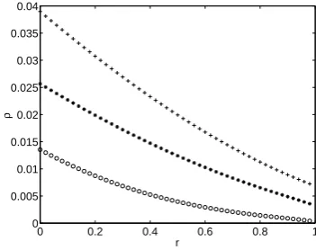
[image:7.595.47.291.161.435.2]

In the following, we make three groups of experiments. In Figure 1, we test the relation betweenρandr, whenn=

100,ω1=ω2=1,r1=r2,α=2,q(m, 1) =3,q(m, 2) =2 and β=1, where “◦′′_{, “}₊′′_{and “}_∗′′_{denotes the spectral radius}

ofP A,〈P A〉and A, respectively. In Table I and Table II, we report the spectral radius of iteration matrices with GPNUSAOR and GNUSAOR. The meaning of notations

ρ(_Hˆ₎_,_ρ₍_H¨₎_and _ρ₍_H₎_{denotes the spectral radius of}_{P A}_,

〈P A〉 and A, respectively.

0 0.2 0.4 0.6 0.8 1

0 0.005 0.01 0.015 0.02 0.025 0.03 0.035 0.04

r

[image:7.595.338.514.285.424.2]

ρ

Fig. 1. The Relation Betweenρandr, Whenn=100,ω1=ω2=1.

From Figure 1, Table I and Table II, we easily see that the preconditioned multisplitting relaxation USAOR methods discussed in this paper substantially have better numerical behaviours than the multisplitting relaxation USAOR methods studied in[9], which shows that our new methods are applicable and efficient.

TABLE I

COMPARISON OFSPECTRALRADIUSWHENα=2,q(m, 1) =2,q(m, 2) =1

n ω1,r1 ω2,r2 β ρ(H˜) ρ(H¨) ρ(H) 50 0.8,0.4 0.7,0.6 0.5 0.0098 0.0211 0.0542 50 1.0,0.6 0.9,0.6 0.8 0.0074 0.0172 0.0437

50 1.0,0.8 1.0,0.7 1 0.0059 0.0154 0.0286 100 0.8,0.4 0.7,0.6 0.5 0.0102 0.0255 0.0563 100 1.0,0.6 0.9,0.6 0.8 0.0085 0.0179 0.0475 100 1.0,0.8 1.0,0.7 1 0.0067 0.0172 0.0304

1000 0.8,0.4 0.7,0.6 0.5 0.0157 0.0312 0.0687 1000 1.0,0.6 0.9,0.6 0.8 0.0105 0.0234 0.0551 1000 1.0,0.8 1.0,0.7 1 0.0089 0.0202 0.0456

ACKNOWLEDGMENT

The authors would like to thank the anonymous ref-erees who made much useful suggestions that helped us to improve the quality of the paper.

IAENG International Journal of Applied Mathematics, 44:1, IJAM_44_1_06

(8)

TABLE II

COMPARISON OFSPECTRALRADIUSWHENα=2,q(m, 1) =3,q(m, 2) =2

n ω1,r1 ω2,r2 β ρ(H˜) ρ(H¨) ρ(H) 50 0.8,0.4 0.7,0.6 0.5 0.0025 0.0123 0.0354 50 1.0,0.6 0.9,0.6 0.8 0.0021 0.0111 0.0298

50 1.0,0.8 1.0,0.7 1 0.0018 0.0095 0.0213 100 0.8,0.4 0.7,0.6 0.5 0.0028 0.0145 0.0388 100 1.0,0.6 0.9,0.6 0.8 0.0026 0.0140 0.0364 100 1.0,0.8 1.0,0.7 1 0.0025 0.0136 0.0325

1000 0.8,0.4 0.7,0.6 0.5 0.0030 0.0151 0.0407 1000 1.0,0.6 0.9,0.6 0.8 0.0029 0.0146 0.0390 1000 1.0,0.8 1.0,0.7 1 0.0027 0.0142 0.0380

REFERENCES

[1] T. Z. Huang, X. Z. Wang, Y. D. Fu, “Improving Jacobi methods for nonnegative H-matrices linear systems,”Appl. Math. Comput.,vol. 186, pp. 1542-1550, 2007.

[2] Y. Zhang, T. Z . Huang, “Modified iterative methods for nonnegative matrices and M-matrices linear systems,”Comput. Math. Appl.,vol. 50, pp. 1587-1602, 2005.

[3] D. Noutsos, M. Tzoumas, “On optimal improvements of classical iterative schemes forZ-matrices,”J. Comput. Appl. Math.,vol. 188, pp. 89-106, 2006.

[4] A. Hadjidimos, D. Noutsos, M. Tzoumas, “More on modifications and improvements of classical iterative schemes for Z-matrices,”

Linear Algebra Appl.,vol. 364, pp. 253-279, 2003.

[5] A. Yasar Ozban, “On accelerated iterative methods for the solution of systems of linear equations,”Int. J. Comput. Math.,vol. 76, pp. 765-773, 2002.

[6] T. Z. Huang, G. H. Cheng, X. Y. Cheng, “Modified SOR-type iterative method for Z-matrices,”Appl. Math. Comput.,vol. 175, pp. 258-268, 2006.

[7] W. Li, “Comparison results for solving preconditioned linear sys-tems,”J. Comput. Appl. Math.,vol. 177, pp. 455-459, 2005.

[8] D. P. O’Leary, R. E. White, “Multisplittings of matrices and parallel solution of linear systems,” SIAM J. Alge. Disc. Math., vol. 6, pp. 630-640, 1985.

[9] L. T. Zhang, T. Z. Huang, et al, “Convergence of relaxed multisplit-ting USAOR methods for H-matrices linear systems,”Appl. Math. Comput.,vol. 202, pp. 121-132, 2008.

[10] Z. Z. Bai, “On the convergence domains of the matrix multisplit-ting relaxed methods for linear systems,” Applied Mathematics J. Chinese University,vol. 13b, No. 1, pp. 45-52, 1998.

[11] Z. H. Cao, Z. Y. Lin, “Convergence of relaxed parallel multisplitting methods with different weighting schemes,”Appl. Math. Comput,

vol. 106, pp. 181-196, 1996.

[12] M. Neumann, R. J. Plemmons, “Convergence of parallel multisplit-ting iterative methods for M-matrices,”Linear Algebra Appl.,vol. 88, pp. 559-573, 1987.

[13] L. Elsner, “Comparisons of weak regular splittings and multisplit-ting methods,”Numer. Math.,vol. 56, pp. 283-289, 1989.

[14] A. Frommer, G. Mayer, “Convergence of relaxed parallel multisplit-ting methods,”Linear Algebra Appl.,vol. 119, pp. 141-152, 1989.

[15] R. E. White, “Multisplitting with different weighting schemes,”

SIAM J. Matrix Anal. Appl.,vol. 10, pp. 481-493, 1989.

[16] D. R. Wang, “On the convergence of the parallel multisplitting AOR algorithm,”Linear Algebra Appl.,vol. 154-156, pp. 473-486, 1991.

[17] R. Bru, V. MigallSn, J. Penadds, D. B. Szyld,“ Parallel synchronous and asynchronous two-stage multisplitting methods,” Electronic Transactions on Numerical Analysis,vol. 3, pp. 24-38, 1995.

[18] D. B. Szyld, “Synchronous and asynchronous two-stage multi-splitting methods,” inProceedings 5th SIAM Conference on Applied Linear Algebra, (J. G. Lewis, Ed.), SIAM, Philadelphia, 1994.pp. 39-44,

[19] J. Mos, D. B. Szyld, “Nonstationary Parallel Relaxed Multisplitting Methods,”Line. Alge. Appl.,vol. 241-243, pp. 733-747, 1996.

[20] A. Berman, R. J. Plemmons, Nonnegative Matrices in the Mathe-matical Sciences,SIAM, Philadelphia, PA, 1994.

[21] R. S. Varga, Matrix Iterative Analysis,Prentice-Hall, Englewood Cliffs, NJ, 1981.

[22] L. Yu. Kolotilina, “Two-sided bounds for the inverse of an H-matrix,”Lin. Alg. Appl.,vol. 225, pp. 117-123, 1995.

[23] M. Benzi, D. B. Szyld, “Existence and uniqueness of splittings for stationary iterative methods with applications to alternating methods,”Numer. Math.vol. 76, pp. 309-321, 1997.

[24] A. J, Li, “A New Preconditioned AOR Iterative Method and Com-parison Theorems for Linear Systems,”IAENG International Journal of Applied Mathematics,vol. 42, no. 3, pp. 161-163, Aug. 2012.

[25] J. Y. Yuan, D. D. Zontini, “Comparison theorems of preconditioned Gauss-Seidel methods for M-matrices,”Appl. Math. Comput.,vol. 219, pp. 1947-1957, 2012.

[26] H. Saberi Najafi, S. A. Edalatpanah, “ Comparison analysis for improving preconditioned SOR-type iterative method,”Nume. Anal. Appl.,vol. 6, no.1. pp. 62-70, 2013.

[27] X. Z. Wang, “Block preconditioned AOR methods for H-matrices linear systems,”J. Comput. Anal. Appl., vol. 15, no.1, pp. 714-721, 2013.

[28] G. B. Wang, T. Wang, F. P. Tan,“Some results on preconditioned GAOR methods,”Appl. Math. Comput., vol. 219, no.11, pp. 5811-5816, 2013.