Thesis

Abstract

1. Introduction

Cap-and-trade systems for carbon emissions and carbon taxes have garnered the most attention as market-based solutions for reducing carbon emissions. However, in the United States at least, these strategies have been politically difficult to implement. Many states have turned, instead, to renewable portfolio standards (RPS), under which the government requires load-serving entities (electric utilities) to procure a certain percentage of their electricity from renewable sources. These standards have been introduced to promote the development of renewable energy sources like wind, solar, biomass, and geothermal. Several states have introduced tradable renewable energy certificates (RECs) to facilitate meeting these standards. Renewable energy certificates are issued to renewable energy generators for each megawatt-hour (MWh) of electricity they produce. These certificates can then be purchased in the REC

marketplace by electric utilities, who can use the certificates to meet their annual RPS requirements. A penalty is imposed on load-serving entities who fail to meet their RPS requirement. The emergence and rapid growth of REC markets suggests that they may be an important policy alternative to emissions trading schemes and carbon taxes.

requirements are fixed and do not vary with the price (Felder and Loxley 2012). Markets for RECs are also characterized by a price floor of zero (renewable energy generators can always choose not to sell their RECs so they would never sell them for a negative price) and a price ceiling equal to the compliance penalty (load-serving entities will never pay more than the penalty for RECs because they can simply pay the penalty instead). Due to the vertical demand curve, small changes in supply can significantly affect prices. Small supply changes are

represented by leftward and rightward shifts of the supply curve for RECs, which is also vertical in the short-run. Theoretically, equilibrium exists only at a price of zero and at a price equal to the penalty with no equilibrium between the two, as shown in Figure 1. If there is an oversupply of RECs, the price will be essentially zero, and if there is an undersupply of RECs the price will equal the penalty fee (Felder and Loxley 2012). Coulon et. al (2015) show that prices for SRECs in New Jersey have fluctuated enough to suggest that REC demand is approximately described by a vertical curve. The short-run supply curve is vertical because renewable energy generators do not choose how much electricity to produce based on price. If the sun is shining or the wind is blowing, renewable generators are producing electricity and creating RECs in the process. In a single period, this electricity production may vary stochastically with weather, but it is

Figure 1. For a single period, REC markets have a vertical demand curve as shown. When there is an undersupply (S1) of certificates, the REC price is equal to the penalty price SACP (solar alternative compliance penalty). When

there is an oversupply (S2) of certificates, the REC price is zero.

In this paper, I propose replacing traditional renewable portfolio standards with emissions rate standards in order to create a downward-sloping demand curve for renewable energy

certificates. A rate standard will require electricity generators to reduce their carbon emissions to a specified amount of carbon dioxide (CO2) per MWh. Under this model, electricity

generators have two choices to meet their emissions rate standard: (1) reduce emissions per MWh through abatement or (2) purchase RECs. I create a theoretical model and use this to show that rate standards will result in a downward-sloping demand curve for RECs. Then I test this model using the dynamic programming algorithm outlined by Coulon et al. (2015) to show that price volatility is reduced relative to New Jersey’s current regulatory model.

Several papers have discussed the price volatility of markets for renewable energy certificates in the United States and for green certificates in Europe. Some have proposed

compliance penalty and adaptive REC requirement that vary with price (Khazaei et al. 2016). Other papers have looked at rate standards as a type of carbon emissions reduction regulations and have compared them to cap-and-trade schemes (Bushnell et al. 2015; Burtraw et al. 2012). However, no paper has examined implementing rate standards as a method of reducing price volatility in renewable energy certificate markets.

My paper contributes to the literature by demonstrating the implementation of emissions rate standards for renewable energy generation is a potential solution for limiting price volatility and making renewable energy a less risky investment. While rate standards are not a new policy, implementing emissions rate standards as a method of reducing price volatility in renewable energy certificate markets is a new idea. The ultimate goal of most environmental markets is to reduce pollution. This is especially true for carbon markets and renewable energy policies. Carbon markets serve to reduce carbon emissions in order to slow climate change. Renewable energy certificate markets and other policies such as portfolio standards and feed-in tariffs serve to encourage the growth of clean energy, which can indirectly result in less emissions from dirty fossil fuel-fired plants as these plants are phased out over time. However, the production of renewable energy does not by itself lead to any decrease in greenhouse gas emissions. By directly linking the generation of renewable energy to carbon emissions through an emissions rate standard, my policy both incentivizes the creation of clean energy and the reduction of carbon dioxide emissions from dirty power producers. Under my policy, electricity producers can choose the most cost-effective method of reaching the rate standard but they must either reduce emissions or buy renewable energy certificates.

(RGGI), a cap-and-trade program for carbon dioxide emissions from electric power plants in the northeastern United States, until 2011 when it withdrew from the program. The CPP gives states the option of reducing emissions through cap-and-trade or rate standards, and since New Jersey has abandoned cap-and-trade, it seems likely that it would turn to rate standards. My policy design is such that New Jersey would only have to modify its existing SREC program to implement rate standards rather than starting a new, separate program for carbon emissions.

The paper proceeds as follows. First, I present a case for why this paper is important by illustrating the existing price volatility in New Jersey’s SREC market. Second, the paper discusses the current literature available on renewable energy certificate markets, New Jersey’s SREC price volatility, similar green certificate markets, and emissions rate standards. Third, I introduce a theoretical model for a single period where the REC requirement and penalty are replaced by an emissions rate standard. In the next section, the demand portion of the model is extended across time, and the SREC generation function presented in Coulon et al. (2015) is used as a model of REC supply. By modifying the dynamic programming algorithm from the same authors to accommodate my demand function, I demonstrate that a rate standard can reduce price volatility in REC markets. This is presented in the results section.

2. Price Volatility in Renewable Energy Certificate (REC) Markets

Data collected on New Jersey’s solar renewable energy certificate (SREC) market demonstrates that prices have rapidly fluctuated since the introduction of certificates in 2005. This price volatility, sometimes in the form of severe price swings, has led to high variation in the creation of new SRECs over time. In other words, price fluctuations are causing

volatility causes high risk to participants in the market for renewable energy certificates and may potentially lead to less investment in renewable power generation.

The supply of certificates in time period 𝑡 depends on the certificate price in time period 𝑡 − 1. The higher the certificate price in the previous period, the greater the renewable

generation capacity installed in the current period. From the perspective of government

regulators, we would like to see relatively stable prices to encourage stable growth of renewable energy generation.

Figure 2. Daily average SREC prices in New Jersey for the period 2007-2015. The dark blue lines indicate the penalty price for each energy year. The different colored lines indicate the prices for SRECs according to the energy year in which they were issued. Data obtained from NJ Clean Energy Program.

Figure 3. Annualized monthly SREC issuance rate over the period 2007-2015. The dark blue lines (dots) indicate the SREC requirement (number of SRECs necessary to meet compliance) for each energy year. Data obtained from

NJ Clean Energy Program.

0 2 0 0 4 0 0 6 0 0 8 0 0 SR EC Pr ice ($ )

7/1/2007 7/1/2009 7/1/2011 7/1/2013 7/1/2015 Date

SACP EY2008 EY2009

EY2010 EY2011 EY2012

EY2013 EY2014 EY2015

Daily Average SREC Prices

0 2 0 0 0 4 0 0 0 6 0 0 0 8 0 0 0 An n u a lize d SR EC I ss u a n ce (1 ,0 0 0 MW h ) 1/1/20071/1/20081/1/20091/1/20101/1/20111/1/20121/1/20131/1/20141/1/2015 Date

Requirement EY2008 EY2009

EY2010 EY2011 EY2012

EY2013 EY2014 EY2015

Figure 4. The blue line graph (left axis) shows the annual growth rate of new solar installations in New Jersey over the period 2008-14. The red bar graph (right axis) shows the average SREC price in the previous year. This figure was obtained from Coulon et al. (2015).

These figures demonstrate that there is clearly a relationship between historical prices of renewable energy certificates and the growth of the solar industry in New Jersey. Since

investment in renewable energy appears to be tied to investors’ expectations of certificate prices, price volatility is a major concern if renewable growth is the ultimate goal. This provides the motivation for my policy proposal to limit price volatility and create stable prices in order to stimulate the renewable energy sector.

3. Literature Review

Coulon et al. (2015) examine the price volatility of New Jersey’s solar renewable energy certificates (SRECs) in the paper “SMART-SREC: A stochastic model of the New Jersey solar renewable energy certificate market.” First, the authors study the price history of New Jersey’s SRECs, accounting for the numerous regulatory changes that have occurred since the

introduction of certificates in 2005. The price history demonstrates that there is a clear

lag present in the market’s response to price movements. Second, the authors build stochastic models called SMART-SREC for SREC prices and for SREC generation. Central to these models is a feedback feature in which the price is a function of generation and the generation model is a function of price. Using New Jersey’s historical price data, the authors estimate the parameters of the models and determine the optimal time lag parameter. This paper’s main contribution is twofold: (1) it shows the high sensitivity of SREC prices to market design and market participant behavior and (2) it proposes a stochastic model with reasonable parameter estimates that replicates historical price movements. I use their stochastic generation model in my paper as a model of certificate generation (or supply) over time. I also replicate, and then adapt, the dynamic programming algorithm these authors use to generate price surfaces for various combinations of certificates banked and certificates generated. Ultimately, the adaptation of this algorithm allows me to prove that my model can reduce price volatility.

In the paper “ADAPT: A Price-stabilizing Compliance Policy for Renewable Energy Certificates,” Khazaei et al. (2016) develop a model for a downward-sloping demand curve as suggested by Felder and Loxley (2012). The model Khazaei et al. create depends on a sloped penalty function, which they call an Adjustable Dynamic Assignment of Penalties and Targets (ADAPT) policy. Under this policy proposal, the penalty price would be a function of the total number of submitted RECs in the energy year and the compliance requirement would be determined based on the size of the certificate surplus or shortage of the previous year. The authors use the same SREC generation model they developed in Coulon et al. (2015). By creating a dynamic programming model and deriving properties of the market, the authors are able to compare how different market designs affect price level and volatility. They conclude that the ADAPT model with a downward-sloping demand curve can significantly reduce price volatility and ensure stable long-run prices (Khazaei et al. 2016).

Amundsen et al. (2006) investigate the extent to which price volatility can be reduced if certificates are allowed to be banked in their paper “Price Volatility and Banking in Green

Certificate Markets.” The authors also study the effects of certificate banking and speculation on consumer, producer, and social surplus. Their findings suggest that banking may considerably reduce price volatility and also lead to increased social surplus (Amundsen et al. 2006).

variable, it is reasonable to prohibit borrowing. This is unlike carbon emissions markets, in which borrowing is allowed because the amount of permits available for the next year is a known quantity. Additionally, failing to meet the certificate requirement in the current year does not imply a certificate debt for the next year because the utility would just pay the penalty fee. This means that banking does not change the upper bound on prices—the penalty fee remains the upper price bound for certificates (Coulon et al. 2015). As a measure by itself, banking does not appear to be the solution for reducing price volatility, although it may help if combined with another measure.

In the EPA’s Clean Power Plan released this year, the EPA calls for significant emissions reductions and sets targets for each state to reach by 2030 (Bushnell et al. 2015). These targets are emissions rate-based CO2 goals, which is the type of standard I am proposing in my paper.

4. Theoretical Model

I develop a theoretical model for the renewable energy certificate market when rate standards are the government-imposed regulation instead of renewable portfolio standards. My theoretical work shows that the rate standard model creates a downward sloping demand curve for RECs and, as a result, limits REC price volatility.

The economic agents in this model are electricity generators—both renewable and non-renewable. We begin with the assumption that renewable power producers and other electricity generators are trying to maximize profits. I start by considering a simple single-period

theoretical model. Later, I extend this model to adjust for additional factors including certificate price history, stochastic renewable energy production, certificate banking.

4.1. Variables and Notation

I use the following notation and variables.

Indices: Time is indexed by t, where one month is the smallest time step (∆𝑡 = 1

12) because New Jersey’s SREC generation data is monthly. The energy year—the year the certificate is used to meet compliance—is indexed by 𝑦 ∈ ℕ. Each of N electricity generators is indexed by i. Prices: The market price of a certificate at time t used to meet compliance in energy year y is denoted 𝑝_{𝑐,𝑡,𝑦}. This price is determined endogenously by my theoretical model in the single-period framework and by the dynamic programming algorithm in the multi-single-period framework. Certificate prices are measured in dollars per certificate ($/REC), where each certificate

electricity. The wholesale price of electricity is measured in dollars per MWh of electricity sold ($/MWh).

Emissions rates: The carbon dioxide emissions rate for electricity generator i is denoted 𝛽𝑖 and is measured in pounds of CO2 per MWh of electricity generated (lbs CO2/MWh). I assume each

firm’s emissions rate is constant over time; any emissions abatement achieved is accounted for in the emissions reduction variable 𝑒𝑟, defined below, so it would be double-counting to include it as a reduction in the actual emissions rate. My proposed policy mechanism, a rate standard set by a regulator, is denoted 𝜎_𝑡 and has units lbs CO2/MWh. In the multi-period model, the rate

standard is modeled by a continuous decreasing function so the standard becomes stricter over time.

Power plant emissions rate data indicates that carbon dioxide emissions rates from power plants on the grid that supplies New Jersey with electricity have not changed much over the past five years. This is shown in the Figure 5. This helps validate the decision to have 𝛽_𝑖 remain constant for each firm in the model. We estimate the average emissions rate across firms 1

𝑁∑ 𝛽𝑖 𝑁

Figure 5. Carbon dioxide emissions rate data from the period 2012-2014 for the PJM Interconnection, which supplies New Jersey's electricity. The gray line, which represents the average emissions rate across all power plants on the grid, indicates that the emissions rate has remained fairly constant at approximately 1,100 pounds of CO2 per

MWh since 2012.

Quantities: The quantity of electricity sold by each generator i in time t is represented by 𝑞_{𝑒,𝑖,𝑡} and is measured in MWh. Similarly, the quantity of certificates sold by each generator i in time t

is represented by 𝑞_{𝑐,𝑖,𝑡} and is measured in RECs where one REC stands for one MWh of electricity production. Note that while all generators sell electricity, only renewable generators create certificates, so 𝑞_{𝑐,𝑖,𝑡} will be zero for all non-renewable generators.

Emissions reductions: Under my model, a firm can buy certificates, reduce emissions, or both in order to meet the rate standard. The emissions reductions achieved by firm i in time t are

Parameters:

 The interest rate is denoted by r. I assume the interest rate is 𝑟 = 0.02 for this paper.

 Each firm faces costs of reducing carbon emissions through abatement. These costs are known as abatement costs. We assume that the marginal abatement cost function is isoelastic with parameter 𝜆. This parameter has units $

(lbs CO2)2.

State variables:

 The installed capacity of SREC generation at time t is denoted 𝑔̂_𝑡.

 The accumulated number of SRECs banked at time t is denoted 𝑏_𝑡. Decision variable:

Each electricity generator chooses how many certificates to submit at each compliance date according to their individual certificate demand functions. They will choose the least costly combination of emissions abatement and RECs. The number of certificates each firm i chooses to submit at time t is denoted 𝑥𝑖,𝑡.

4.2. Constraint: Carbon Emissions Rate Standard

New Jersey currently sets a fixed requirement for the amount of solar-generated electricity a utility must produce each year, or, in other words, the number of SRECs that must be submitted each year. I remove this requirement on utilities and instead place a rate standard requirement on electricity producers. In order to create a downward-sloping demand curve, I propose an

emissions rate standard of the form below that will act as a constraint on dirty electricity producers.

This standard is set such that 𝜎 < 𝛽̅, so a significant number of electricity producers will be required to reduce their emissions to meet the standard. Firms whose emissions rates are higher than the standard (𝛽𝑖 > 𝜎) must either buy certificates (increase 𝑞𝑐,𝑖) or abate carbon dioxide emissions (increase 𝑒_𝑟,𝑖). Under this policy, each REC directly offsets one MWh of electricity production from dirty power sources. Similarly, one unit of emissions reduction (pound of CO2)

directly offsets one unit of emissions production. A generator’s total emissions, accounting for these offsets, is then divided by the quantity of electricity it produces 𝑞𝑒,𝑖, and it must be equal to or less than the mandatory emissions rate standard. Firms whose emissions rates are lower than the standard (𝛽_𝑖 < 𝜎) are in compliance and they do not have to perform any additional action. The rate standard above assumes electricity producers have the ability to abate emissions. It also assumes that the quantity of electricity produced by each firm is constant and determined

exogenously from this decision about how many certificates to buy and how much pollution to abate. Considering that a majority of producers who fail to meet the rate standard are baseload producers, it is reasonable to assume their electricity production is fixed.

We check this functional form to ensure that reducing emissions and buying certificates allow a firm to meet the rate standard. Consider the function below

𝑓(𝑞_𝑐,𝑖, 𝑒_𝑟,𝑖) =𝛽𝑖(𝑞𝑒,𝑖− 𝑞𝑐,𝑖) − 𝑒𝑟,𝑖 𝑞_𝑒,𝑖

where 𝑓(𝑞_𝑐,𝑖, 𝑒_𝑟,𝑖) describes firm i’s actual emissions rate taking into account the certificates it

has purchased 𝑞_𝑐,𝑖 and the emissions it has abated 𝑒_𝑟,𝑖. Then taking the partial derivatives, we have

𝜕𝑓 𝜕𝑞_𝑐,𝑖 = −

𝛽_𝑖

𝑞_𝑒,𝑖 and 𝜕𝑓 𝜕𝑒_𝑟,𝑖 = −

Both partial derivatives are negative, which indicates increasing the number of certificates a firm purchases or increasing a firm’s emissions reductions will cause the firm’s effective emissions rate to decrease. In other words, a firm whose emissions rate is higher than the standard 𝜎 can meet the standard by buying certificates or abating emissions (or both).

4.3. Electricity Generators

In order to create a demand function for RECs, we begin with the assumption that electricity producers are profit-maximizing firms. In this scenario, electricity production is exogenously determined and firms are choosing how many certificates to buy and how much to abate. The profit maximization problem for such a firm is below.

max 𝑞𝑐,𝑖,𝑒𝑟,𝑖

(𝑝_𝑒𝑞_𝑒,𝑖 − 𝐶_𝑖(𝑞_𝑒,𝑖) − 𝐶(𝑞_𝑐,𝑖, 𝑒_𝑟.𝑖))

The first cost function in this model, 𝐶_𝑖(𝑞_𝑒,𝑖), is the cost of producing electricity, which I assume is quadratic

𝐶𝑖(𝑞𝑒,𝑖) = 1 2𝑞𝑒,𝑖

2

Then the profit maximization problem becomes

max 𝑞𝑐,𝑖,𝑒𝑟,𝑖

(𝑝_𝑒𝑞_𝑒,𝑖−1 2𝑞𝑒,𝑖

2 _{− 𝐶(𝑞}

𝑐,𝑖, 𝑒𝑟.𝑖))

The remaining cost function in this problem includes the costs of buying RECs and the costs of reducing emissions. It has the form

𝐶(𝑞_𝑐,𝑖, 𝑒_𝑟.𝑖) = 𝐴𝐶(𝑒_𝑟,𝑖) + 𝑝_𝑐𝑞_𝑐,𝑖

reducing pollution by one additional unit. For simplicity, I assume the generator’s marginal abatement cost function is isoelastic with parameter 𝜆. In other words, 𝑀𝐴𝐶(𝑒_𝑟,𝑖) = 𝑒_𝑟,𝑖𝜆 . Thus,

𝐴𝐶(𝑒_𝑟,𝑖) = ∫ 𝑀𝐴𝐶(𝑒_𝑟,𝑖)𝑑𝑒_𝑟,𝑖 𝑒𝑟,𝑖

0

= ∫ 𝑒_𝑟,𝑖𝜆 𝑑𝑒_𝑟,𝑖 𝑒𝑟,𝑖

0

Additionally, we can rewrite the emissions constraint 𝜎 =𝛽𝑖(𝑞𝑒,𝑖−𝑞𝑐,𝑖)−𝑒𝑟,𝑖

𝑞_𝑒,𝑖 in terms of 𝑒𝑟,𝑖. 𝑒_𝑟,𝑖 = 𝛽_𝑖(𝑞_𝑒,𝑖− 𝑞_𝑐,𝑖)− 𝜎𝑞_𝑒,𝑖

Then the generator’s abatement cost function becomes

𝐴𝐶(𝛽_𝑖(𝑞_𝑒,𝑖− 𝑞_𝑐,𝑖)− 𝜎𝑞_𝑒,𝑖) = ∫ 𝑒_𝑟,𝑖𝜆 𝑑𝑒_𝑟,𝑖 𝛽_𝑖(𝑞_𝑒,𝑖−𝑞_𝑐,𝑖)−𝜎𝑞_𝑒,𝑖

0

This allows us to rewrite the firm’s costs as a function of only the quantity of certificates it purchases.

𝐶(𝑞_𝑐,𝑖) = ∫ 𝑒_𝑟,𝑖𝜆 𝑑𝑒_𝑟,𝑖 𝛽_𝑖(𝑞_𝑒,𝑖−𝑞_𝑐,𝑖)−𝜎𝑞_𝑒,𝑖

0

+ 𝑝_𝑐𝑞_𝑐,𝑖

Because the quantity of electricity produced is exogenous, maximizing a generator’s profits is equivalent to minimizing its costs.

min 𝑞𝑐,𝑖

(∫ 𝑒_𝑟,𝑖𝜆 𝑑𝑒𝑟,𝑖 𝛽_𝑖(𝑞_𝑒,𝑖−𝑞_𝑐,𝑖)−𝜎𝑞_𝑒,𝑖

0

+ 𝑝𝑐𝑞𝑐,𝑖)

Therefore, we take the first order condition and solve for 𝑞_𝑐,𝑖.

𝑞_𝑐,𝑖 =

𝑞𝑒,𝑖(𝛽𝑖 − 𝜎) − (𝑝_𝛽𝑐 𝑖)

1 𝜆

𝛽_𝑖

𝑞̅ =𝑐 𝑞𝑒

̅̅̅(𝛽̅ − 𝜎) − (𝑝𝑐 𝛽̅)

1 𝜆 ̅

𝛽̅

To find the aggregate demand function for certificates, we sum the individual demand over all N

electricity generators, or instead we simply multiply this average individual demand by N.

𝐷 = ∑ 𝑞_𝑐,𝑖 𝑁

𝑖=1

= 𝑁𝑞̅ = 𝑁_𝑐 𝑞_𝑒

̅̅̅(𝛽̅ − 𝜎) − (𝑝𝑐 𝛽̅)

1 𝜆 ̅

𝛽̅ =

𝑄_𝑒(𝛽̅ − 𝜎) − 𝑁 (𝑝𝑐 𝛽̅)

1 𝜆 ̅

𝛽̅

where 𝑄𝑒 is the total amount of electricity produced (MWh) in the single period.

From this we can also solve for the inverse demand function where 𝑄𝑐 is the total number of certificates produced in a single period.

𝑝_𝑐 = 𝛽̅ (𝑄𝑒(𝛽̅ − 𝜎) − 𝛽̅𝑄𝑐

𝑁 )

𝜆

We graph this function, which is downward sloping, in the following section.

4.4. Equilibrium

For the purposes of a single-period model, we can assume the supply of certificates is fixed, as renewable energy producers cannot increase or decrease production based on certificate prices. Rather, the short-term supply of renewable electricity is determined only by natural processes (the availability of sunlight, weather patterns, etc.). Generators cannot install more production capacity in a single period, so we consider the supply fixed. In order to obtain an equilibrium price, we can set this fixed supply 𝑆 = 𝑥 equal to demand, which we defined above.

𝑆 = 𝑥 =

𝑄𝑒(𝛽̅ − 𝜎) − 𝑁 (𝑝𝑐 𝛽̅)

1 𝜆 ̅

We obtain

𝑝_𝑐 = 𝛽̅ (𝑄𝑒(𝛽̅ − 𝜎) − 𝛽̅𝑥

𝑁 )

𝜆

We can glean a few pieces of information from this function. First, certificate price responds inversely to changes in the emissions rate standard 𝜎. Lowering the rate standard (making the requirement stricter) causes the price of certificates to increase.

Figure 6. Downward sloping demand curve for certificates. Note this demand curve assumes 𝜆 = 1. This assumption makes graphing easier but is not necessary to produce a downward sloping curve. The curve will be downward sloping regardless of the choice of 𝜆.

For practical policy purposes, this equilibrium condition allows regulators to predict the price of certificates for a certain period based on the rate standard they set if they know the current average emissions rate 𝛽̅ of utilities, the quantity of electricity demanded, the number of renewable and non-renewable electricity generators, and the parameter 𝜆 of the marginal

generators would likely overestimate their costs in order to see a less strict emissions rate standard.

5. Multi-period Model

The purpose of this paper is to show that emissions rate standards can be applied to New Jersey’s SREC market to reduce price volatility of certificates over time. So far, we have only shown that a rate standard produces a downward-sloping demand curve for certificates in a single period. In order to determine if price volatility may be reduced, we extend our demand function across time and follow the methods of the SMART-SREC paper by Coulon et al. (2015) to examine price surfaces at different points in time. The certificate demand function, from Section 4.3, becomes

𝑥_𝑡 =

𝑄_𝑒(𝛽̅ − 𝜎_𝑡) − 𝑁_𝑡(𝑝𝑐,𝑡 𝛽̅ )

1 𝜆 ̅

𝛽̅

where 𝑥_𝑡 represents the number of certificates submitted to meet compliance at time t. We assume total electricity demand 𝑄𝑒 is constant across years, which is not unreasonable based on historical data. Additionally, I design the emissions rate standard 𝜎𝑡 to decrease 2 percent each year in order to achieve environmental policy goals of significantly reducing carbon dioxide emissions. The functional form for 𝜎_𝑡 is

𝜎𝑡 = 0.98𝑡 12⁄ 𝛽̅

Certificates will only be submitted at compliance dates (when 𝑡

Coulon et al. (2015) observe that SREC generation is driven by stochastic processes and they develop a model for the generation of certificates 𝑔_𝑡 (SREC/year):

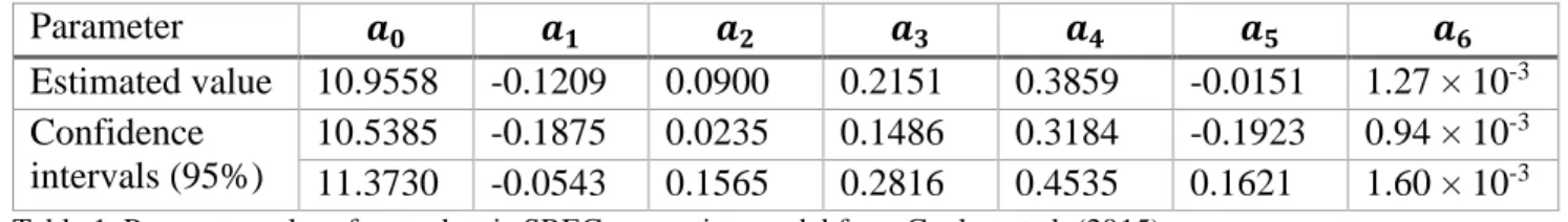
ln(𝑔𝑡) = 𝑎0+ 𝑎1sin(4𝜋𝑡) + 𝑎2cos(4𝜋𝑡) + 𝑎3sin(2𝜋𝑡) + 𝑎4cos(2𝜋𝑡) + 𝑎5𝑡 + 𝑎6∫ 𝑝̅̅̅𝑢d𝑢 𝑡

0

+ 𝜀𝑡

This is simply a model of the supply of SRECs each year. The sine and cosine functions in this model capture the seasonality of SREC generation and the feedback price 𝑝̅𝑡 represents some increasing function of historical prices. In other words, SREC generation varies according to daylight and weather conditions. Generation also depends on SREC market prices, as higher recent prices lead to increased installation capacity of solar power. The last term 𝜀𝑡 represents noise and is estimated to be normally distributed with mean 0 and variance 0.035

(𝜀𝑡~𝑁(0,0.035)). Coulon et al. (2015) estimate the parameters 𝑎0,…,𝑎6, and these estimates are

presented in Table 1.

Parameter 𝒂_𝟎 𝒂_𝟏 𝒂_𝟐 𝒂_𝟑 𝒂_𝟒 𝒂_𝟓 𝒂_𝟔

Estimated value 10.9558 -0.1209 0.0900 0.2151 0.3859 -0.0151 1.27 × 10-3 Confidence

intervals (95%)

10.5385 -0.1875 0.0235 0.1486 0.3184 -0.1923 0.94 × 10-3

11.3730 -0.0543 0.1565 0.2816 0.4535 0.1621 1.60 × 10-3

Table 1. Parameter values for stochastic SREC generation model from Coulon et al. (2015).

The generation model for the annualized instantaneous generation rate 𝑔_𝑡 can be rewritten by exponentiating each side of the equation to obtain

𝑔𝑡 = 𝑔̂𝑡(𝑝) exp(𝑎1𝑠𝑖 𝑛(4𝜋𝑡) + 𝑎2𝑐𝑜𝑠(4𝜋𝑡) + 𝑎3𝑠𝑖𝑛(2𝜋𝑡) + 𝑎4𝑐𝑜𝑠(2𝜋𝑡) + 𝜀𝑡) where 𝑔̂_𝑡 is the installed generation at time t and it evolves according to

𝑔̂_{𝑡+𝛥𝑡} = 𝑔̂_𝑡exp(𝑎₅𝛥𝑡 + 𝑎₆𝑝_𝑡𝛥𝑡).

𝑏_𝑡 = {

max (0, 𝑏_𝑡−1+ ∫ 𝑔_𝑢𝑑𝑢 𝑡

𝑡−𝑡

− 𝑥_𝑡) , 𝑡 ∈ ℕ

𝑏⌈𝑡⌉−1+ ∫ 𝑔𝑢𝑑𝑢 𝑡

⌈𝑡⌉−1

, 𝑡 ∉ ℕ

Recall that certificates are submitted for compliance at the end of each energy year (when 𝑡 ∈ ℕ). Thus, the first line of this function indicates the number of certificates banked just after the certificates (𝑥𝑡) are submitted for compliance. The second line is the sum of the certificates banked from previous years and the number generated so far in the current year.

Whereas the current model and the model proposed in ADAPT by Khazaei et al. (2016) rely on a penalty function, my model only relies on the rate standard. However, in order to simulate my model using those authors’ algorithm, I rewrite my demand function as an alternative to the penalty function.

𝑓_𝑡𝑑𝑒𝑚𝑎𝑛𝑑_(𝑥

𝑡) = {𝛽̅ (

𝑄𝑒(𝛽̅ − 𝜎) − 𝛽̅𝑥𝑡

𝑁 )

𝜆

, 𝑡 ∈ ℕ 0, 𝑡 ∉ ℕ The price of SRECs of vintage year y at time t then satisfies

𝑝𝑡,𝑦 = {max(𝑓𝑡

𝑑𝑒𝑚𝑎𝑛𝑑_(𝑥

𝑡), 𝑒−𝑟𝛥𝑡𝔼𝑡[𝑝𝑡+𝛥𝑡,𝑦]) , 𝑡 ≤ 𝑦 + 𝜏 0, 𝑡 > 𝑦 + 𝜏

Recall the vintage year is the energy year in which the certificate was issued. With a lengthy banking period of five years allowed before a certificate expires, it is highly unlikely that a firm would hold onto a certificate long enough for it to expire. When it is time to meet compliance, a firm will submit its oldest certificates first (this is known as the first in, first out “FIFO” principle and is proved in Khazaei et al. (2016)). This means that the possibility of the price of a

5.1. Dynamic Programming Algorithm

I follow the method described in SMART-SREC by Coulon et al. (2015) and in ADAPT by Khazaei et al. (2016) to examine price volatility. First, I tested the algorithm to ensure that it would replicate the results of those two papers. The algorithm for solving for the price surface at each unit in time works as follows. I begin by discretizing space in the dimensions of 𝑏_𝑡 and 𝑔_𝑡 by choosing a grid of values for those state variables, and I discretize time in monthly steps for a five-year period. I similarly discretize the Normal distribution of the noise 𝜀_𝑡. Then I initialize the program by evaluating the price of an SREC at the end if its five-year life. The algorithm then works backwards through time, solving the martingale condition at each grid point: 𝑝𝑡,𝑦= 𝑒−𝑟𝛥𝑡𝔼𝑡[𝑝𝑡+𝛥𝑡,𝑦]. Matlab’s root finding function “fzero” is used to iteratively solve this

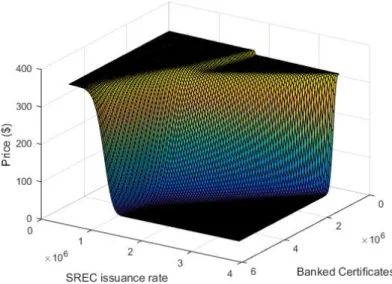
fixed-point problem (Coulon et al. 2015). Figure 7 shows a price surface generated by the algorithm for a given month under New Jersey’s current regulations. The price surfaces at various times t of SREC prices based on my model and generated by the dynamic programming algorithm are presented in Figure 8.

These price surfaces show that SREC prices are much more stable over time, ranging between $95 to $100 per certificate, under my policy proposal than currently in New Jersey where prices range from $0 to that year’s penalty price. Prices do not drop to zero until just months before the certificate is due to expire. However, certificates this old will likely have been submitted for compliance by this time, so the likelihood of the price actually reaching zero is slim. These results suggest that price volatility would be reduced by implementing an emissions rate standard for renewable energy certificates. This is further demonstrated by Figures 9 and 10. Figure 9 shows the simulated price of certificates over a five-year period based on the current regulatory scheme in New Jersey. Figure 10 shows the simulated certificate price over the same period with my rate standard mechanism replacing the existing regulation.

Figure 10. Certificate price over time using my model. Under the rate standard policy, the average monthly price (blue) has a much smaller range from $95 to $100.

According to these simulations, price volatility appears to be significantly reduced under a rate standard policy (Figure 9) compared to New Jersey’s current regulatory scheme (Figure 8). Furthermore, these graphs display the average monthly prices, so prices are likely much more volatile than the averages indicate. The minimum and maximum monthly prices are important in this regard because the prices range between those bounds, which are much closer to each other under the rate standard proposal. In other words, the rate standard appears to set tight restrictions on the range and volatility of certificate prices, which is the result we were looking for.

One important caveat is the long-term generation growth rate and the generation function’s parameter values, all of which were adapted from Coulon et al. (2015), may

6. Conclusion

New Jersey’s SREC market is a leading model for renewable energy certificate markets in the United States. Other states and regions will be looking to New Jersey to see how it deals with price volatility in this market. Policymakers and researchers continue to search for optimal regulatory policies to reduce price fluctuations in certificate markets, and so far New Jersey has been one of several testing grounds for such policies. As renewable energy certificate markets and similar markets continue to grow as a method of incentivizing renewable energy production in order to combat climate change, solving the volatility problem will become even more important.

In my paper, I have proposed a potential solution to this problem. I propose

implementing an emissions rate standard for carbon dioxide emissions that electricity generators can meet by buying renewable energy certificates. Simulations of my model based on the dynamic programming algorithm found in the SMART-SREC paper by Coulon et al. (2015) suggest that REC price volatility is reduced under a rate standard. More research is necessary to confirm this finding, but my work gives good indications that replacing a fixed requirement and penalty function with an emissions rate standard would create in a downward-sloping demand curve for certificates and result in less price volatility. Reducing price volatility is important for potential investors in renewable energy who see stable prices as an encouraging sign of lower risk.

Acknowledgements

Works Cited

Amundsen, Eirik S., Fridrik M. Baldursson. 2006. “Price Volatility and Banking in Green Certificate Markets.” Environmental & Resource Economics 35 (4): 259–87. doi:10.1007/s10640-006-9015-1.

Burtraw, Dallas, Arthur G. Fraas, and Nathan D. Richardson. 2012. “Tradable Standards for Clean Air Act Carbon Policy.” SSRN Scholarly Paper ID 2004401. Rochester, NY: Social Science Research Network. http://papers.ssrn.com/abstract=2004401.

Bushnell, James B., Stephen P. Holland, Jonathan E. Hughes, and Christopher R. Knittel. 2015. “Strategic Policy Choice in State-Level Regulation: The EPA’s Clean Power Plan.” Working Paper 21259. National Bureau of Economic Research.

http://www.nber.org/papers/w21259.

Coulon, Michael, Javad Khazaei, and Warren B. Powell. 2015. “SMART-SREC: A Stochastic Model of the New Jersey Solar Renewable Energy Certificate Market.” Journal of

Environmental Economics and Management 73 (September): 13–31.

doi:10.1016/j.jeem.2015.05.004.

Felder, Frank A., and Colin J. Loxley. 2012. “The Implications of a Vertical Demand Curve in Solar Renewable Portfolio Standards.” Center for Research in Regulated Industries,

Rutgers University, 17.

http://ceeep.rutgers.edu/wp-content/uploads/2013/11/VerticalDemandCurve.pdf.

Khazaei, Javad, Warren B. Powell, and Michael Coulon. 2016. “ADAPT: A Price-Stabilizing Compliance Policy for Renewable Energy Certificates: The Case of SREC Markets.” Working Paper.