Thesis

(1)

Introduction

The study of light harvesting polymer assemblies is of particular interest in the field of solar energy conversion due to their efficient absorption of visible light that can be used to facilitate electron or energy transfer between donors and acceptors to a reaction center to drive catalysis for solar fuel generation. While electron and energy transfer have been well studied in small systems consisting of only a few components, large assemblies comprised of multiple donors and

acceptors give rise to energy and electron transfer dynamics not observed in smaller systems. These polymer structures are disordered and fluctuate on time scales similar to these quenching processes, producing a distribution of time-‐ dependent donor-‐acceptor distances that subsequently result in a distribution of time-‐dependent energy and electron transfer rates. The focus of my undergraduate research has focused on constructing accurate macromolecular models of polymer assemblies that can be used for understanding these photoinduced dynamics in combination with ultrafast spectroscopic results.

The combination of increasingly advanced computational techniques and the reduction in cost of hardware components have allowed greater access to the field of computational chemistry without requiring high levels of expertise in

programming and related fields. Computational chemistry offers a wide variety of tools and methods for creating fully-‐atomistic models of various sizes. For small systems, ab initio methods can be used to produce highly accurate results at the cost of computational resources. Larger systems can be simulated using classical

molecular mechanics that still give reasonable results for moderate computation time.

(2)

representing a distinct part of the polymer structure. The goal of this is to reduce complex full atomistic structures into simpler structures that can run for longer simulation times while using the same amount of computational resources. Over the course of my research, many polymer models have been created and simulated, falling into the general categories of Ru-‐Polystyrene and Ru-‐ Polyfluorene homopolymers as well as an OPE-‐TBT-‐Polystyrene co-‐polymer. The OPE-‐TBT co-‐polymer contained oligo(phenylene-‐vinylene) (OPE) and thiophene-‐ benzothiadiazole-‐thiophene (TBT) pendants attached to styrene repeat units. All Ru polymer models were simulated in an amorphous cell environment with PF6-‐ as the counter-‐ion to balance charge and acetonitrile (MeCN) as the solvent while the OPE-‐ TBT co-‐polymer simulations used tetrahydrofuran (THF) as a solvent instead of acetonitrile. Since OPE and TBT fragments are neutral, no counter-‐ions were needed to balance charge. Molecular dynamics simulations were run up to the nanosecond timescales to better understand the movement of chromophores as they evolved with time.

All simulations and data analysis were done primarily with the software package Materials Studio by BIOVIA (formerly Accelyrs) using the modules

(3)

Figure 1. Structures of monomer units for OPE-‐TBT, Ru-‐Polystyrene, Ru-‐ Polyfluorene.

OC8H17

C8H17O N S N S S S OPE TBT N Ru N N N N N II O NH N N N N N N NH O N Ru N N N N N

C7H15

(4)

Methods and Procedures

Polymer Construction

All polymers, solvents, and various structures of the OPE-‐TBT, Ru-‐

Polystyrene and Ru-‐Polyfluorene models for both atomistic and coarse-‐grain models were drawn in Materials Studio using the available drawing tools. While each

system was unique, they all shared similar construction, optimization and modeling methods. To begin construction a new .xsd file was created and named. Drawing tools allowed for the placement of both single atoms and bonds and simple structures such as aromatic rings. Helpful tools in this process included the add-‐ hydrogen and clean tools. The add-‐hydrogen tool adds hydrogen atoms to all atoms based on missing atoms and the Lewis theory of bonding. The clean tool quickly approximates bond angles and lengths in a structure that can be used for starting calculations.

After building a structure, like a polymer monomer, but before DFT calculations were done to determine the charges, a geometry optimization was performed. This was done to find the structure’s lowest possible starting energy. This optimization uses classical molecular mechanics compared to quantum mechanics for DFT. Geometry optimizations were started by going to the Forcite Calculation tab in the Forcite module and setting the task to “Geometry

Optimization”.

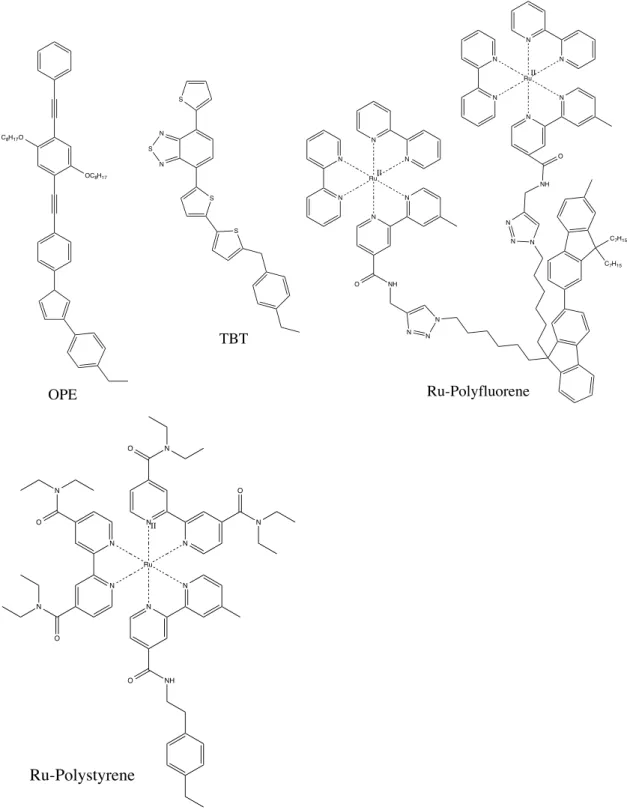
Parameter Setting

Force field Universal

Algorithm Smart

Iterations ~1000-‐10000

Quality Medium

(5)

Figure 2. Evolution of polymer energy during geometry optimization.

Now that the structure had been optimized the charges of individual atoms had to be calculated. Initial tutorial models used the Energy task in Forcite to calculate atomistic charges because of its more user-‐friendly nature for beginners but for OPE-‐TBT, Ru-‐Polystyrene and Ru-‐Polyfluorene, the Gaussian module in Materials Studio was used. Gaussian was chosen because of a wide variety of customizable parameters and reputation within the community and literature.

Parameter Setting

Method DFT

Basis set LANL2DZ

Exchange-‐correlation B3LYP

Properties Electron density, Population analysis

Charge 0 – (OPE/TBT, solvent)

+2 – (Ru-‐PS) +4 – (PF-‐Ru) -‐1 – Counter-‐ion

Table 2. Typical parameters used during geometry optimization process.

(6)

personal computer. The .ginf file was then opened and modified to resemble the following script.

%chk=PFT-‐Ru.chk %Mem=400MB

%nprocshared=8 (12 for killdevil)

#p RHF/B3LYP/Integral(Grid=UltraFine)/Lanl2DZ OPT=(Redundant,Tight)

GEOM(PrintInputOrient) Density Pop(Regular) NoSymm

PFT-‐Ru(II)Geometry Optimization 4 1

Atom’s Cartesian Coordinates

Figure 3. Typical script and parameters used during DFT calculations.

The job was then submitted to run on the cluster using the following commands. 1. Load Gaussian module

module load gaussian/09b01 or 09c01 2. Submit the job to the cluster.

bsub -‐q week –n 8 –R “span[hosts=1]” g09 PFT-‐Ru.chk

After confirming that the Gaussian job had successfully terminated the output .log file was transferred to the appropriate Material Studio folder and the file type was changed from .log to .gof (gaussian output file) so Materials Studio could interpret the results. The structure was then updated by going to the Gaussian Analysis module, selecting analysis and updating the structure and assigning the charges under population analysis.

After optimizing the individual monomers they could finally be built into a polymer. The repeat unit of the polymer was established by designating head and tail atoms and a chiral center if needed by going to the build tab and selecting “repeat unit” under build polymer. The charges of the head and tail atoms were set to zero by selecting them and going to the charges section under the Modify tab, since they would be replaced by connecting monomer units. The remaining

(7)

the structure. This rescaled all the atomistic charges to appropriate values so they all summed to the desired total charge. With the monomer appropriately configured the polymer can now be built by going to the build tab and selecting homopolymer under build polymer. The defined repeat unit was selected from possible structures and the number of repeat units was defined. All polymers had their Tacticity set to Atactic and the torsion of the individual units was set to random. Building a co-‐ polymer like the OPE-‐TBT polymer required the use of a probability matrix that was defined under the co-‐polymer tab.

Probability of Next Unit

OPE TBT

Current Unit OPE 0.9 0.1

TBT 1.0 0.0

Table 3. Example of probability matrix used for construction of co-‐polymer.

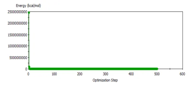
The next step of the process, before cell construction, was to anneal the polymers. In the annealing process the polymers were artificially heated to a certain temperature ~700-‐800 K and then cooled back down to around room temperature, ~300 K. The purpose of this was to make sure the polymer was at its absolute energy minimum and not a local minima as could be the case using a geometry optimization.

Figure 4. Energy graph showing annealing process to reach global energy minimum.

Parameter Setting

Annealing cycles 5

Initial Temperature 300 K

Mid-‐cycle Temperature 700 K

(8)

Dynamics steps per ramp 200

Time step 1.0 fs

Ensemble NVT

Table 4. Table 1. Typical parameters used during annealing process.

The ensemble specifies that the cell will have constant mass (N), constant volume (V), and constant temperature (T). Additionally the cell was set to optimize after each cycle, using the same values as the geometry optimization steps. The total number of dynamics steps could be calculated by multiplying together the number of annealing cycles, heating ramps per cycle times two and the dynamics steps per. This was multiplied by the time step to determine the total time of the simulation. Time steps were generally required to be less than 1.5 fs otherwise it would result in unsuccessful termination of the annealing job. As a general rule, the time step can’t be larger than ~1/10th_{the frequency of high frequency vibrations such C-‐H} stretching at 3000 cm-‐1_{(11 fs), otherwise energy deviations prevent the structure} from converging.

Figure 5. Temperature profile vs. time for an amorphous cell with Ru-‐Polyfluorene during annealing process. Profile shows 5 distinct annealing cycles, oscillating cell between low and high temperatures.

(9)

Cell Construction, Annealing and Dynamics

After building, optimizing and annealing the polymers, they were then placed into an amorphous cell using the Amorphous Cell module in Materials Studio. Two separate methods used to place the polymers in a solvent environment or

amorphous cell. In the first method, the Construction task, predefined quantities of polymer, solvent, and counter-‐ions were used to construct a cell. The cells were set to have periodic boundary conditions to simulate a bulk substance. The second method, a slight variation of the first, used the Packing task. It was developed because often times the job would fail because no suitable configuration could be found for both the large polymer and large quantity of solvent. A cell was

constructed first with only predefined quantities of polymer and counter-‐ion. After running the construction the cell was resized with each side being ~35-‐40 A. The cell was then packed with solvent. If the polymer in the cell showed unusual configuration another geometry optimization was run. All cells were set to have a cubic structure.

The next step in the process, before beginning molecular dynamics, was to anneal the entire cell. This was traditionally done using the kure or killdevil cluster since running an annealing job of this size could take up to several days. The desired .xsd file was then transferred to the cluster along with two additional files, a script.x and ex.pl file required to successfully run the annealing job. The script.x file contains instructions for the cluster on how to run the job while the .pl file, a Perl script, holds the specific parameters of the annealing job. The .pl file should have the same name as the .xsd file. All three files had to placed within the same folder in the cluster to run successfully. To submit the job the following commands were typed into the Secure Shell command prompt.

3. To execute the script.x file

chmod +x script.x

4. Convert windows files to unix.

dos2unix *

5. Submit the job to the cluster.

(10)

ex is the name of the .xsd/.pl file being used.

After checking that the job had successfully completed, by opening the .txt file and seeing if it terminated normally, all files were downloaded from the cluster into a new Materials Studio folder. The annealing process in the cell could be observed visually by opening the ex.xtd file and using the animation toolbar.

At this point, depending on the project, the next step would’ve been to start molecular dynamics or pull low energy structures from the annealing process and use them as the basis of molecular dynamics. The annealing process would often terminate at an intermediate temperature, resulting in a cell that wasn’t at its energy minimum. Individual frames, containing the amorphous cell, were extracted from the .xtd file by opening the Forcite module and selecting analysis. The “view in study table” option at the bottom allows each individual frame to be extracted to make a new .xsd file. For large .xtd files, creating a study with each frame present can be computationally demanding so only frames containing minimum energy structures were selected. This could be done by either visual inspection of the Temperature.xcd file, one of the original output files, or by using Temperature analysis tool in Forcite Analysis to get the frame numbers. In the create study table tab the frame numbers were entered into the “frames” box after selecting the correct trajectory file and opening the trajectory specification box next to it and entering the numbers separated by commas and the include structures box was selected. The amorphous cells were extracted from the table by double-‐clicking the desired cell in the structures column to display it and right clicking in the black space and selecting to extract it from the study table. This creates an .xod file, by right clicking the black space again and selecting to create a new atomistic .xsd file. Using the appropriate .xsd file molecular dynamics simulations were started by going to the Forcite module, selecting Forcite Calculation and changing the task to “Dynamics”. Additional parameters were set depending on the specific

requirements of the simulation and the goals of the project. The options in the Dynamics settings allowed for simulation time to be input directly.

(11)

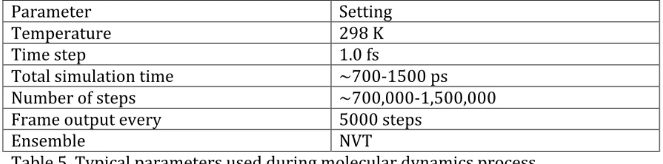
Parameter Setting

Temperature 298 K

Time step 1.0 fs

Total simulation time ~700-‐1500 ps

Number of steps ~700,000-‐1,500,000

Frame output every 5000 steps

Ensemble NVT

Table 5. Typical parameters used during molecular dynamics process.

The same ensemble was used for both annealing and dynamics jobs to ensure consistency of results. While these jobs were observed to be less computationally expensive compared to annealing jobs they were still often very demanding for a personal computer and so they were often run on the cluster, either kure or killdevil. The process was the exact compared to submitting annealing jobs to cluster except a different .pl file, containing dynamics instructions, was used. Molecular dynamics simulations often required several days or even a full week of computing time to run, even on the cluster. Dynamics simulations could be

continued by either extracting the last frame of the dynamics .xtd file using the same process or checking the restart box in the Forcite Calculation window when the “Dynamics” task is selected. Dynamics simulations were often restarted several times for each polymer type so total simulation time could be built up into nanosecond time scales, between ~2-‐10 ns.

(12)

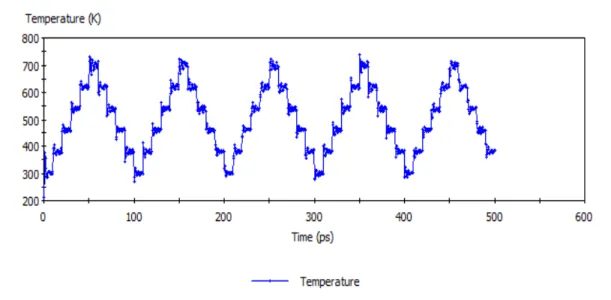
Figure 6. Temperature profile vs. time for an amorphous cell with Ru-‐Polyfluorene during molecular dynamics. Compared to annealing process, dynamics shows small random temperature variations.

Data Acquisition

The main goal of molecular dynamics simulations of all polymers was to track the spatial movement of chromophores as they evolved throughout the simulation. This included measuring chromophore-‐chromophore distances, chromophore-‐backbone distances, and the mapping of Cartesian coordinates. Distance measurements were taken by selecting the distance tool in the Materials Studio toolbar and selecting the two atoms of interest in the polymer or cell, creating a visual distance measurement. Multiple measurements were made this way to create a complex web of distance measurements within the polymer. Individual or groups of measurements were hidden by selecting the desired

measurements, right clicking in empty space, selecting the measurements tab under display style, and changing the measurements display style to “None”. The actual measurements were extracted from .xsd/.xtd file by selecting the models tab in the Materials Studio toolbar and selecting “Distance measurements” to run. Doing this requires a study table for the .xsd/.xtd file of interest. The measurements are

returned as an array in the study table that can be separated by right clicking on the column heading and selecting “Split Arrays”. At this point results were copied and pasted into an Excel or Origin spreadsheet for plotting and further analysis. These measurements were often used to create distance vs. time plots by copying and pasting the time column into the Excel/Origin sheet to observe whether the distance measurements were still fluctuating or had begun to equilibrate.

(13)

composed the polymer backbone. Analysis of the coordinates was then done in Origin to create 3D scatter plots, showing how the positions of either the Ru(II) atoms or the backbone changed during the annealing and molecular dynamics process.

Mesocite – Coarse-‐Grain Modeling

Coarse-‐grain models of the polymer Ru-‐Polyfluorene and its amorphous cell were created and simulated using the Mesocite module and its corresponding toolbar in Materials Studio. A 35-‐unit Ru-‐Polyfluorene polymer was used for all molecular dynamics simulations, not including solvent simulations. The polymer, solvent and counter-‐ion had already been coarse-‐grained, individual focus was on creating and amorphous cell and beginning molecular dynamics. A mesostructure can’t be created using the procedure as the full atomistic models. The cell was made by selecting Mesostructure Template from the Materials Studio toolbar, setting the cell to have the proper size (X ~100 A, Y ~ 25 A, Z ~25 A) and then adding and assigning a filler to the cell. Next the polymer was copied and pasted into the cell. Next the build mesostructure tool was selected, solvent and counter-‐ion were added and their relative quantities set, along with the cell density, creating a coarse-‐

grained amorphous cell. The cell was then optimized using the geometry optimization task in the Mesocite module. Molecular dynamics were started by going to the Mesocite module and setting the task to dynamics. The same

parameters used in Forcite full atomistic simulations were used for the Mesocite simulations except the total simulation time was changed to run for tens/hundreds of nanoseconds. Coarse-‐grain simulations also took several days or a week to run and terminate normally using the above timescales.

Results

Gaussian – DFT Calculations

(14)

were achieved. These results serve mostly to help with various troubleshooting issues encountered during the process. The computational runs involving Ru-‐ Polyfluorene would terminate in error due having to solve for the interactions between two charged metal ions. Three separate methods were explored to overcome this problem.

#p RHF/B3LYP/Integral(Grid=UltraFine)/Lanl2DZ SCF=QC (or XQC)

OPT=(Redundant,Tight) GEOM(PrintInputOrient) Density Pop(Regular) NoSymm

The above script uses a different method to converge on a final energy using the keywords QC or XQC. Both of these methods can be applied generally on all structures such as monomer units, solvents and counter-‐ions. The main drawback using this method is that using QC or XQC for convergence significantly increases computational time, although the algorithm is generally more reliable.

#p RHF/B3LYP/Integral(Grid=UltraFine)/Lanl2DZ SCF

SCRF=(PCM,Solvent=Acetonitrile) OPT=(Redundant,Tight)

(15)

resulted in lower computational runtimes. Like the above method though, a drawback to using this method is it requires significant memory usage.

#p RHF/B3LYP/Integral(Grid=UltraFine)/Lanl2DZ SCF=QC (or XQC)

The final script removes the geometry optimization steps and simply calculates the atomistic charges. This was used specifically in cases where after analyzing the output file in Molden to see whether the energy had begun to converge it was determined that the structure had optimized close enough to its final geometry. This structure could then be imported into a new input file and have the charges calculated.

Additionally, for several different results involving Ru-‐Polyfluorene the calculation would successfully terminate, but when the .gof file was imported into Materials Studio the option to update structure would work but the charges couldn’t be assigned in population analysis. Several different methods were tried to

overcome this with the most successful and consistent result being to select “natural population analysis” under Gaussian Calculation when setting up the calculation.

(16)

Forcite – Full Atomistic Simulations

Figure 7. 30 unit OPE-‐TBT co-‐polymer colored to show OPE (orange), TBT (blue) and the polymer backbone.

Figure 8. 20 unit Ru-‐Polystyrene polymer without hydrogen’s attached.

(17)

Figure 9. 8 unit Ru-‐Polyfluorene polymer without hydrogen’s attached.

Initial models using the OPE-‐TBT copolymer were packed with ~2500 molecules of THF solvent for a 30 unit system. This was determined to be too computationally expensive due to the higher number of molecules that had to be simulated in addition to the polymer. The large number of solvent molecules were required because large cells were initially constructed to prevent the interaction with polymers from adjacent cells affecting dynamics. Future simulations generally maintained ~500 molecules of solvent for all polymer types since this offered a good compromise between computational time and cell size. The choice of solvent was also an important consideration during cell construction. The OPE-‐TBT simulations that used THF as a solvent were generally more computationally

(18)

Figure 10. Amorphous cell composed of 8 unit Ru-‐Polyfluorene polymer with the solvent acetonitrile and PF6-‐ counter-‐ion. Solvent is contained in cell before dispersing during annealing and molecular dynamics simulations.

The main concern in keeping reasonable computational was because of the need to build up simulation time in the molecular dynamics. The goal was to simulate the polymers as they relaxed from the annealing process and reached equilibrium. This included observing the individual chromophores in the polymer to see if they reached and equilibrium configuration. Other areas of interest included measuring chromophore-‐chromophore distances and determining the chromophore closest to the backbone as a function of time. These simple scatter plots were

(19)

Graph 1. Scatter plot of distance between two Ru(II)atoms in 3-‐Polyfluorene polymer as a function of time.

Graph 2. Distance-‐distribution profiles of OPE-‐TBT distances in OPE-‐TBT co-‐

polymer.

The distance distributions represent the most probable distance between OPE donors and TBT acceptors. Studying the distance distributions between donors and acceptors was part of a larger series of experiments to study the rate of energy transfer between chromophores within the polymer. Further analysis of OPE-‐TBT co-‐polymer will be included with Ru(II)polymers later in the discussion.

More advanced 3D scatter plots were created using Origin to observe the spatial positions of the Ru(II) atoms and the polymer backbone as they evolved through the simulation time.

20 22 24 26 28 30

0 100 200 300 400 500 600

D ist an ce ( A )

Time (ps)

Ru-‐Ru Distance

-‐1 0 1 2 3

0 5 10 15 20 25 30 35

Pr

ob

ab

ili

ty

(20)

Figure 11. 3D scatter plot of backbone atoms in 8 unit Ru-‐Polyfluorene polymer.

(21)

Figure 12. 3D scatter plots of Ru(II)atoms in 3 unit Ru-‐Polyfluorene (left) and 20 unit Ru-‐Polystyrene (right) undergoing annealing process.

Ru-‐Polystyrene on the other hand with its clumped, twisted backbone meant

(22)

Figure 13. 3D scatter plots of Ru(II)atoms in 3 unit Ru-‐Polyfluorene (left) and 20 unit Ru-‐Polystyrene (right) undergoing molecular dynamics process.

The overarching goal of these polymer models is to help provide insight into the underlying dynamics that govern the polymers. Two specific physical processes were being looked at; electron transfer and energy transfer from a donor

chromophore to an acceptor after photoexcitation occurred. Electron transfer and energy transfer are in direct competition with each other so understanding the physical processes that govern both is an important step in developing materials designed to favor one of these processes. The model used to describe this long-‐ range energy transfer is the Forster resonance energy transfer (FRET), which uses the following equations to calculate the rate of energy transfer. In FRET energy is transferred from donor to acceptor by the excited state donor electron relaxing and using the energy to excite an acceptor electron.

1

𝜏_!"# = 1 𝜏_!(

𝑅_!

𝑅)!

R is simply the distance between donor and acceptor chromophores, so energy transfer within the polymer will be less efficient over long distances.

𝑅_! = 9000ln10𝜙! 128𝜋!_𝑛!_𝑁 𝐽(𝜆)

(23)

electron to an acceptor that then exchanges a ground state electron with the donor, thereby transferring energy between donor and acceptor. The process is considered efficient compared to Forster energy transfer.

𝑘_!" ∝𝐽(𝜆)𝑒!!!/!

L is simply the sum of the van der Waals radii between donor and acceptor.

𝐽 𝜆 = 𝐹!(𝜆)𝜀!(𝜆)𝜆!𝑑𝜆

!

The integral is the spectral overlap integral, which represents the total area of overlap between the absorbance spectrums of the donor and acceptor

chromophores. The larger this integral is the faster energy transfer will occur, assuming all other parameters remain constant.

In a recent publication that this research contributed to, in Accounts of Chemical Research, the spectral overlap integral of several Ru(II)polymers was measured and analyzed to determine its correlation to the composition of the backbone. The polymers analyzed were Ru-‐PF (polyfluorene), Ru-‐PFT

(24)

Figure 14. Structures of Ru(II)monomers for Ru-‐PF, Ru-‐PFT, Ru-‐PF2T and Ru-‐PT with number of monomer units.

Results showed that increasing the thiophene composition of the polymer backbone steadily red-‐shifted the absorbance spectrum of the acceptor chromophore, as shown in the below figure. This in turn led to red-‐shifted donor emission and hence an overall reduction in the overlap integral.

(25)

Figure 15. Emission spectrum for donor (gray) and absorbance spectrum for

acceptor (blue) chromophores with shaded region representing area of overlap.

Since electron transfer is in direct competition with energy transfer, a

reduction in the energy transfer rate will make electron transfer the more favorable process. The study shows how the chemical structure of a system can be modified to selectively favor one physical process over another by tuning the composition of the backbone. For systems with tightly packed chromophores, like Ru-‐PT which has a smaller backbone compared to Ru-‐PF, multiple acceptors can interact and

participate increasing the rate of electron and energy transfer compared to a simple donor-‐acceptor system.

The molecular dynamics simulations were used in conjunction with

experimental data to help understand photoinduced dynamics and electron transfer within the polymer with focus toward the development of solar energy conversion applications. By studying energy transfer within polymers, this could help lead to potentially viable, new solar collection methods for future energy use. New solar collection technologies are of critical interest today because solar energy is both highly abundant and can be adapted to suit a wide variety of functions, from large energy collection facilities to catalyzing chemical reactions.

(26)

Figure 16. Full atomistic representation of Ru-‐Polyfluorene (left) and coarse-‐grain model (right).

(27)

Figure 17. Coarse-‐grain model of 35 unit Ru-‐Polyfluorene polymer used for

molecular dynamics simulations.

Additionally the coarse-‐grain model was set to have a simulated time of

tens/hundreds of nanoseconds while the full atomistic model could only achieve picosecond/nanosecond timescales using the same computational resources.

Figure 18. Temperature profile vs. time for an amorphous cell with Ru-‐Polyfluorene during molecular dynamics using coarse-‐grain models.

(28)

The were several disadvantages of using coarse-‐grain models though. The Mesocite module lacks an annealing task so constructed cells can’t be annealed, leaving only geometry optimization to relax the structure. It was also observed that during the simulation that bonds in the polymer would quickly expand to

unreasonable valuables, negating the simulation. Different methods to correct this problem were attempted, including restraining bonds and changing the force field type of the beads that composed the polymer coarse-‐grain model. Attempts to

restrain the bonds lengths resulted in forced reduction of the time step, reducing the simulated time to full atomistic level. This resulted in coarse-‐grain models providing mixed results compared to full atomistic models. Properly classifying force field types on the individual beads though resulted in coarse-‐grain models that were more consistent with previous simulation results.

Conclusion

(29)

solved before they can be used to help interpret experimental data about the modeled system.

The basis for these polymer systems was to help interpret experimental data to understand complex physical phenomena like energy transfer within the

polymer. Understanding this is of interest because of the potential light harvesting applications of these polymers. Further development in the field of these polymers could lead to new classes of solar collection devices. Given current demands for new energy modeling of polymers will continue to play a role in research for the

foreseeable future.

(30)

Scripts

Shell Script #!/bin/sh -‐x

export WORKDIR=`pwd` cd $WORKDIR

for host in $LSB_HOSTS do

echo $host

done > ./machines.LINUX

export DSD_MachineList=$WORKDIR/machines.LINUX export DSD_NumProc=1

# this is for Killdevil

export MPI_ROOT=/nas02/apps/materialstudio-‐6.0/killdevil/MaterialsStudio6.0/ /nas02/apps/materialstudio-‐

6.0/killdevil/MaterialsStudio6.0/etc/MatServer/bin/RunMatServer.sh -‐np $DSD_NumProc $1

Anneal Script #!perl

use strict;

use MaterialsScript qw(:all);

use File::Copy;

my $doc = Documents-‐>Import("PF2T.xtd");

Modules-‐>Forcite-‐>Calculation-‐>Run($doc, Settings(Task => "Anneal", TimeStep => 1.0, AnnealCycles => 5, InitialTemperature => 300.0, MidCycleTemperature => 700.0, StepsPerRamp => 20000, CurrentForcefield => "Universal", ChargeAssignment => "Use current", EnergyDeviation => 2000000 ));

Dynamics Script #!perl

use strict;

use File::Copy;

(31)

Modules-‐>Forcite-‐>Dynamics-‐>Run($doc, Settings(Ensemble3D => "NVT", TimeStep => 0.5, NumberOfSteps => 40000, TrajectoryFrequency => 500, CurrentForcefield => "Universal", ChargeAssignment => "Use current", EnergyDeviation => 2000000000));

Script for Extraction of Cartesian Coordinates #!perl

use strict;

use Getopt::Long;

#open the multiframe trajectory structure file or die my $doc = $Documents{"./20-‐Polystyrene.xtd"};

if (!$doc) {die "no document";}

my $trajectory = $doc-‐>Trajectory;

if ($trajectory-‐>NumFrames>1) { # Open new report file

my $report=Documents-‐>New("xtd2xmol.txt");

$report-‐>Append("Found ".$trajectory-‐>NumFrames." frames in the trajectory\n"); $report-‐>Close;

# Open new xmol trajectory file

my $xmolFile=Documents-‐>New("trj.txt");

#get atoms in the structure