Thesis

(1)

Health Shocks and Retirement Timing in Latin America

By

Laura Sale

Honors Thesis

Economics Department

The University of North Carolina at Chapel Hill

March 2016

Approved:

_______________________________

(2)

Abstract:

In this paper, I analyze the health and demographic factors that influence the timing of

retrirement. I use pooled data from six Latin American countries and investigate cross-country

variations in retirement age and response to health shocks. I examine the effects of heart attacks,

strokes, and cancer as well as two measures of overall health status on the population as a whole,

divided based on demographic characteristics, and before and after nationwide pension reforms. I

make use of childhood events and characteristics as instrumental variables to attempt to control

for the endogeneity of health shocks in my model. I find that heart attacks, strokes, and cancer

diagnoses have a strong effect on the retirement hazard that varies little across demographic

(3)

Acknowledgements

I would like to thank Dr. David Guilkey, my excellent advisor, and Dr. Klara Peter for

the help and encouragement they have provided throughout this process. I could not have

completed this process without Dr. Guilkey’s guidance in developing and reworking my research

question, his knowledge, support and patience. I am grateful to Dr. Peter for the skills she taught

(4)

I. Introduction

The age of retirement is a matter of growing concern in Latin America. A recent article in

the New York Times1 reported that early workforce exit is quickly becoming a crisis in Brazil, a country in which the average age of retirement is 54. The combination of early retirement,

generous benefits—Brazilian public officials often receive pensions totaling over $100,000 per

year—and increasing lifespans is draining public funds and spurring intense political debate. The

problem is particularly troublesome in Brazil, one of the few remaining Latin American

countries with a pay-as-you-go public pension scheme, but funding early retirement is an issue

that extends to much of Latin America and the Caribbean, where the population has been aging

and labor force participation has been declining among older age groups since the middle of the

20th century.2

Latin America’s declining rates of labor force participation among older individuals

mirrors trends that have occurred in developed countries including the United States in the later

part of the 20th century. While the trends have been similar, residents of most Latin American

and Caribbean countries retire earlier than their counterparts in other regions. The average age at

which retired respondents in the database I am using, the Survey on Health, Well-being, and

Aging in Latin America and the Caribbean (SABE), left the workforce was 55. For comparison,

the current average age of retirement in the US is 62, although it has varied over the years,

dropping as low as 57 in the period 1991-1993.3 It is important to understand the early average

age of retirement Latin America, a regional phenomenon that has not received very much

attention in the economics literature and could have serious consequences for the growth of these

(5)

economies. Additionally, the distributions of the retirement age in many of these countries are

quite broad: there are significant numbers of people who continue working until advanced ages

as well as a large number who retire very early in life.

In response to fiscal difficulties posed by aging populations and early retirement as well

as the precarious financial situations of elderly populations, many Latin American countries

implemented pension reforms in the 1980s and 1990s. The most significant of these changes

involved a transition from pay-as-you-go funding of retirement pensions to individual retirement

accounts. The impact of these reforms is uncertain, but expected to help relieve the states’

financial troubles and potentially reduce the level of economic security retirees can expect to

attain. The countries in my dataset that replaced their pay-as-you-go system with individual

retirement accounts are Argentina, Chile, Mexico, and Uruguay. These developments have the

potential to alter the incentives involved in retirement, and therefore could impact the timing of

workforce exit. I attempt to assess the effect that Latin American pension reform has had on

retirement.

The remainder of this paper is divided into five sections. I begin with a review of

literature in the health and retirement fields as it pertains to my research. In the third section, I

explain the theoretical model of health and retirement that I use as the basis of my understanding.

Next I discuss the dataset I am using that comes from responses to the Survey on Health,

Well-being, and Aging in Latin America and the Caribbean. In section four, I describe my empirical

(6)

II. Literature Review

There has been substantial research done on the financial incentives that impact

retirement decisions including salary and expected income from social security and pensions.

van Erp, et al.found that non-financial determinants including social norms, default options, and

reference-dependent utility are also significant.4 Existing research on the relationship between

health and retirement has found that poor health tends to reduce the age at which people retire.

Kuhn, et al. hypothesized that health influences the timing of workforce exit through its effects

on morbidity and on the disutility of work. Having better health implies that an individual has a

later expected time of death, necessitating the accumulation of more savings before retirement.

Additionally, worse health increases the disutility of work, making retirement a more attractive

option. The authors conclude that, in general, poor health should reduce individuals’ age of

retirement.5

Research on health and retirement in Latin America is fairly limited. Barrientos, whose

research studies Chileans over the age of 55, found that many people continue working until an

advanced age. He attributed this to the high degree of financial vulnerability experienced by

households headed by older individuals, making labor income a necessary form of

diversification, and to the high degree of income wealth and income inequality among people

over the age of 55. He predicted that Chile’s 1980 pension reform, which moved from a

pay-as-you-go system to individual retirement accounts would increase this vulnerability since the

individual accounts will be more susceptible to labor market fluctuations and will involve less

wealth redistribution. He concluded that these reforms would likely force those who are already

working until advanced ages to remain in the labor force even longer.

4_{Van Erp, et al. “Non-financial Determinants of Retirement.”}

(7)

The evidence from other Latin American countries on the effects of pension reform is

conflicting. A review of the work in this area reveals evidence of divergent effects between

countries. In 1995, Uruguay introduced pension reform which reduced the incentives to retire

early by expanding the range of benefits awarded and tying benefits more closely to

contributions and years in the workforce. Forteza and Sanroman found that the new policy had

little effect on retirement decisions6. Very few people elected to remain in the labor force longer.

Other studies, however, find that generosity of pension schemes does play an important role in

retirement decisions. Aguila concluded that the financial incentives to retire at an early age

created by the Mexican social security program are important contributors to retirement choices,

especially among members of the lower portion of the income distribution7.

There is a fascinating body of research on the relationship between subjective and

objective measurements of health. Atlas and Skinner found evidence that education and

economic factors have an impact on the perception of and likelihood of reporting pain. The

authors also noted that social norms may play a role in pain perception and that there exist data

suggesting that pain perception increases in response to generous disability programs8. In

contrast, Benitez-Silva et al. found that self-reported measures of health are fairly unbiased in the

context of disability insurance9. Waidmann et al. described the presence of psychological factors

that affect self-reported health, suggesting that the decline in self-reported health among

Americans over the age of 60 in the 1970s could be a result of improvements in disability

programs. The authors attribute this effect to justification bias and the potential for employment

to change individuals’ perception of their own health. Waidmann et al. also hypothesized that the

6

Forteza and Sanroman, “Social Security and Retirement in Uruguay.”

7_{Aguila, “Male Labor Force Participation and Social Security in Mexico.”} 8_{Atlas and Skinner, “Education and the Prevalence of Pain.”}

(8)

increase in prevalence of poor self-reported health could have been due to the increase in

screenings and early diagnoses, causing people to adopt a more negative attitude toward their

health status10.

The effects described are important because perceived health is believed to be an

important factor in the decision of whether or not to remain in the labor force. Bound found that

subjective measures of health are a stronger predictor of retirement than are certain objective

measures, which may not be a good measurement of work-capacity11. My data includes

subjective, self-assessed health as well as a composite health score based on a variety of tests and

questions.

In addition to the effect of health on workforce exit, there is also evidence for a causal

relationship running in the opposite direction. Eibich found that retirement can have a positive

effect on health status and mental health. Eibich attributed this change to a reduction of

job-related stress and an increase in hours devoted to sleep and exercise12. The timing of changes in

health status and retirement are important since an improvement in health resulting from

retirement creates reverse causality. This makes it difficult to estimate the effect of health on

retirement without panel data. I incorporate incidences of heart attacks, strokes, and cancer as

time-variant health variables in my hazard model to help overcome this problem.

10_{Waidmann, et al. “The Illusion of Failure.”}

(9)

III. Theoretical Model

My theoretical model is a lifetime utility maximization model based on Mitchell and

Fields’s model of retirement.13

The present value of lifetime income can be represented by the

following equation:

𝐼𝑖 = ∑ 𝑤𝑖,𝑡𝛿𝑡+ 𝑅

𝑡=0

∑ 𝑝𝑖,𝑡𝛿𝑡 𝑇

𝑡=𝑅

Here, 𝑤_𝑡 is the wage earned in period t, 𝑝_𝑡 is the value of income received as transfers from

pension plans and social security payments. 𝑅 is the time of retirement and the primary choice

variable. 𝑇 is the time of death, which is determined by the law of motion of the stock of health

described below, following Grossman’s (1972) model. 𝛿 is a discount factor to account for the

fact that people tend to value future income and expenditures as less highly than present income

and expenditures.

We then have that lifetime utility is a function of the present value of lifetime income,

leisure defined as the number of years between exiting the workforce and death (𝑇 − 𝑅), and

health, which individuals value for its effect on enjoyment of leisure time as well as good

health’s positive effect on income.

𝑈_𝑖 = 𝑓₁(𝐼_𝑖, 𝑇 − 𝑅, 𝐻_𝑖,𝑡 )

Individuals choose the age at which they will retire, 𝑅, in order to maximize lifetime

utility. The optimal value of 𝑅 can increase or decrease with wage earned depending on the

relative magnitudes of the disutility of labor and the utility of consumption, and decreases with

the quantity of income expected from retirement plans.

An individual’s health stock, 𝐻𝑡, follows the law of motion

(10)

𝐻𝑡 = (1 − 𝛿𝑡)𝐻𝑡−1+ 𝑓2(𝑀𝑡−1, 𝐸) + 𝜀𝑡

The model can accommodate a constant rate of depreciation of health or one that varies over

time. 𝑀_𝑡 represents the per period investment made in health-improving activities or care. 𝑓₂ is a

function describing the improvement made to health which takes as its inputs health care

investments and the individual’s education, 𝐸, which is assumed to improve the efficiency with

which an individual produces health. Shocks to health, such as disease or injury, enter the health

function through the error term, 𝜀_𝑡. The individual dies when 𝐻_𝑡 = 0, by construction at time 𝑇.

It is expected that declining health increases the hazard of retirement. Poor health both

reduces the average number of days an individual can work, thereby reducing the return to being

employed (the wage) and increases the disutility of working. Therefore, we would expect to find

a negative relationship between health and age of retirement.

IV. Data

The data set that I am using for this project is The Survey on Health, Well-being, and

Aging in Latin America and the Caribbean (SABE). It is supported by the Inter-university

Consortium for Political and Social Research. Interviews of 11,226 individuals aged 60 and older

were conducted between 1999 and 2000 in Brazil, Argentina, Cuba, Chile, Barbados, Mexico,

and Uruguay. All respondents were residents of urban areas. Respondents were asked a series of

questions pertaining to their health, living situation, childhood illnesses and living situation,

employment or reason for not being employed, medical history, difficulty performing daily

living activities, income from work and other sources, etc. In addition, respondents’ cognitive

and physical capabilities were assessed through a number of tests. If a respondent was deemed

(11)

summary statistics for key variables. I supplemented the SABE dataset with a variable,

individuals’ composite health score, from the RELATE data set14

that McEniry, another

researcher working with SABE as a subset of her data. This variable is based on the Short-Form

12, an overall measure of functional health and well-being widely regarded as valid and

consistent. The SF-12 is comprised of 12 questions assessing self-reported health, BMI, frailty,

and functionality. McEniry’s version, modified to include only the objective measures of health,

drops self-reported health from the calculation and re-weights the output using only the questions

that assess the remaining factors. Additionally, I merge this data set with information on the

pension and social security reforms obtained from the United States Social Security

Administration.

Figure 1 depicts the age of retirement by country. For all countries except Barbados, the

median age of retirement is 60 or younger. Across the countries surveyed the average age of

retirement is 55.19. It should be noted, however, that 2,503 of the 11,226 respondents had not

retired at the time of the survey. The average age of those remaining in the labor force is 65, so

the mean retirement age of 55.19 in my sample is biased downwards from the true population

value. Nonetheless, residents of the countries in my sample are retiring earlier than their

counterparts in other countries. The average retirement age for Americans in the period

1995-2000 was 62.15 Additionally, a sizeable portion of the population retires at a very young age.

10% leave the workforce at or before the age of 29. People who stop working at such a young

age likely leave the workforce for reasons that are very different than those who leave the

workforce later in life. I consider this to be a different decision from the one that I am attempting

(12)

to analyze, and so in my estimation, I include only respondents who remained in the workforce

until at least age 35.

There are disparities in retirement age across demographic groups. Self-assessed health,

gender, country of residence, type of employment, race, household size, and other factors likely

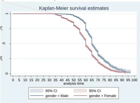
affect the age at which people choose to leave the workforce. Figure 2 shows the differences in

retirement patterns between men and women. Women have a significantly higher hazard of

retirement (a lower probability of survival) at every age than men do. For the countries in my

dataset, the official retirement age for women is 60 and 65 for men. This explains the drops in

survival hazards that occur at age 60 and 65 for women and men, respectively. The other, smaller

drops at five year intervals may suggest that there is some rounding error in respondents’ reports

of the age at which they retired.

Figure 3 gives the survival hazard compared among three countries, Brazil, Cuba, and

Mexico. There are significant differences in retirement patterns between these countries. On

average, Cubans retire earlier than their Brazilian and Mexican counterparts. The retirement age

in Brazil and Mexico has a larger variance, possibly due to unequal access to pensions and social

assistance. Pension payments in Brazil, in particular, are highly unequal across employment

sectors, with government officials receiving far higher pensions than private sector workers.

Figure 4 demonstrates that there is some difference in retirement patterns dependent upon

the educational level attained by a worker.

In order to estimate my model, I transformed the cross-sectional data into survival

format. The data I work with is a person-age dataset with an observation for each person who

held a job every year from the age of 35 to the time of retirement. This allows me to analyze the

(13)

V. Empirical Model

I use data in the panel format discussed in the previous section in order to estimate the

hazard of retiring at each age. Based on self-reported age at workforce exit, I create a dummy

variable, 𝑅_𝑖,𝑡 representing retirement in year t conditional upon not retiring in year t-1.

𝑅𝑖,𝑡 = {0 𝑖𝑓 𝑖 𝑑𝑖𝑑 𝑛𝑜𝑡 𝑟𝑒𝑡𝑖𝑟𝑒 𝑖𝑛 𝑦𝑒𝑎𝑟 𝑡_{1 𝑖𝑓 𝑖 𝑑𝑖𝑑 𝑟𝑒𝑡𝑖𝑟𝑒 𝑖𝑛 𝑦𝑒𝑎𝑟 𝑡} . 𝑟𝑒𝑡𝑖𝑟𝑒 is the variable of interest. A small number of

individuals (approximately 1%) reported retiring at an age older than their age at the time of the

survey. I have excluded these observations from my estimation.

My base empirical model is a single spell discrete time hazard model in which the

outcome of interest is probability of retirement. In order to predict the probability that an

individual i will retire in period t, I use logit estimation on an equation of the form

(1) 𝑙𝑛 [𝑃(𝑅𝑖,𝑡=1|𝑅𝑖,𝑡−1=0)

𝑃(𝑅𝑖,𝑡=0|𝑅𝑖,𝑡−1=0)] = 𝛽𝑋𝑖,𝑡+ 𝛼1𝑠𝑟. ℎ𝑒𝑎𝑙𝑡ℎ𝑖 + 𝛼2𝑜𝑏𝑗. ℎ𝑒𝑎𝑙𝑡ℎ𝑖 + 𝛼2𝑐𝑜𝑢𝑛𝑡𝑟𝑦𝑖 +

𝛼₃ℎ𝑒𝑎𝑙𝑡ℎ𝑠ℎ𝑜𝑐𝑘_𝑖,𝑡+ 𝛼₄𝑡𝑖. ℎ𝑒𝑎𝑙𝑡ℎ𝑠ℎ𝑜𝑐𝑘_𝑖,𝑡 + 𝜇_𝑖

Here, the dependent variable is the log odds that individual i will in year t conditional on i

having not retired prior to year t. 𝑋_𝑖,𝑡 is the vector of time-specific controls, including age, age

squared, race, years of education, and whether or not individual i smokes. Since all individuals

are observed from the age of 35, including age in my regression accounts for duration

dependence. _irepresents time-invariant unobservable characteristics that affect an individual’s

timing of the retirement decision. Such factors could include motivation, job satisfaction, and

other preferences.

My key variables of interest are health factors: 𝑠𝑟. ℎ𝑒𝑎𝑙𝑡ℎ_𝑖, 𝑜𝑏𝑗. ℎ𝑒𝑎𝑙𝑡ℎ_𝑖, ℎ𝑒𝑎𝑙𝑡ℎ𝑠ℎ𝑜𝑐𝑘_𝑖,𝑡,

and 𝑡𝑖. ℎ𝑒𝑎𝑙𝑡ℎ𝑠ℎ𝑜𝑐𝑘𝑖,𝑡. 𝑜𝑏𝑗. ℎ𝑒𝑎𝑙𝑡ℎ𝑖 is the composite health score, an objective measure of

(14)

Survey participants rated their health as either poor, fair, good, very good, or excellent. The

variable ℎ𝑒𝑎𝑙𝑡ℎ𝑠ℎ𝑜𝑐𝑘_𝑖,𝑡 represents three categories of shocks to an individual’s health: heart

attacks, stroke, and cancer.

Based on my theoretical model, I expect to find that measurements of health are inversely

related to probability of retirement while health shocks have a positive effect on the hazard of

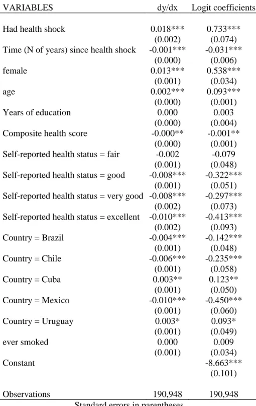
retirement. Results from the base regression are reported in Table 2.

The variable with the largest impact on workforce exit is health shocks, with a highly

significant marginal effect of .018, implying that experiencing a heart attack, stroke, or receiving

a cancer diagnosis increases one’s likelihood of retiring by 1.8% at the mean. The negative

coefficient on years since a health shock implies that over time, the effect of a health shock on

the probability of retiring gradually dissipates. Additionally, self-reported health appears to be

stronger predictor of retirement than does the objective measure, which does not have a

statistically significant marginal effect.

Country of residence also affects age-specific probability of retirement. Brazilians and

Chileans are likely to retire later than workers in the other countries in the dataset. The base

category for race is white. People who identify as mestizo, mulatto, or black tend to retire at a

later age than workers identifying as other races. Women tend to retire at an earlier age than

men, most likely as a result of the asymmetric official retirement ages and possibly of cultural

norms in Latin America and the Caribbean.

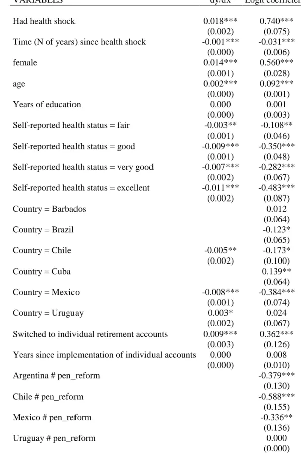
Pension Reform

An important factor that is not accounted for in my base regression is the availability of

(15)

security regulations, I included a pension policy dummy variable, indicating a national switch

from a pay-as-you-go funding scheme to individual retirement accounts. The results of this

regression are found in Table 3. I find that pension reform has a significant effect on propensity

to retire. On average, the introduction of individual retirement accounts as a replacement for

pay-as-you-go funded pensions increased the hazard of workforce exit by .9%. Additionally, I

included an interaction term between health shocks and pension reform. I do not find that reform

had a significant impact on propensity to retire in the face of a health shock. People seem to

respond similarly to heart attacks, strokes, and cancer no matter the structure of their pension

plans.

That pension reform increased the hazard of retirement is a surprising result. Barrientos

(2000) wrote that Chile’s 1980 pension reform, which mirrors the changes made in the other

countries in my sample, would have the effect of making retirement riskier16. The individual

retirement accounts would involve risky investments and would have less of a redistributive

effect on wealth. Accordingly, potential retirees would be forced to remain in the labor force

longer as labor income would become a more important source of risk diversification. My results

suggest that people tend to retire earlier once individual retirement accounts are established. This

suggests that the reforms may have reduced the risk raced by workers considering retirement.

That people are retiring earlier however, may mean that the changes will not bring about the

intended effect on state budgets and economic growth.

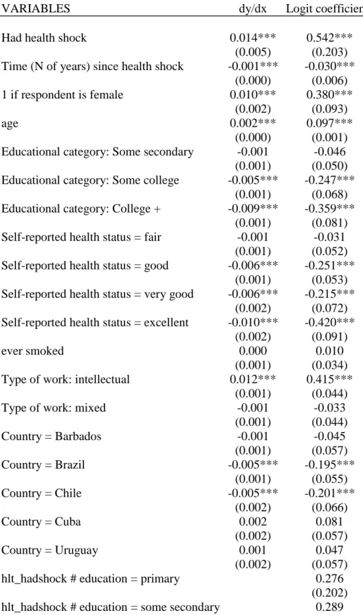
Differences by Demographic Characteristics

A second area of interest is the relationship between health shocks and certain

demographic characteristics. My third regression includes interaction terms between education

(16)

and health shocks and between gender and health shocks. Table 4 reports the results of this

estimation. The negative coefficients associated with having at least some college education

indicate that more educated workers are likely to retire later than less educated workers. Further,

I find that college-educated workers are more likely to retire in response to a health shock than

are workers with less education. This suggests that while more educated workers are willing or

able to continue working until more advanced ages, they may have the luxury of being able to

leave the workforce if they experience a physical decline brought on by a heart attack, stroke, or

cancer diagnosis. The effect of education on response to a health shock does not become

significant until a worker has attended college. My estimation also suggests that health shocks

have differing effects on men and women. Women are more likely to respond to a health shock

by retiring than are men.

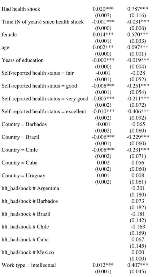
Since country of residence was shown to be important to the timing of retirement, I also

examined the interaction of country of residence and health shocks. The regression output is

found in Table 5. None of these coefficients however were statistically significant in the

specification that I used. Country of residence impacts retirement decisions, but I could not

conclude that it has an additional impact on retirement when a health shock has occurred. Health

shocks have fairly symmetric effects across countries and pension schemes, possibly because

their effect on retirement timing is strong enough to nearly override other considerations in most

cases.

Based on this regression, we can see that the type of work done also impacts the decision

to retire. The base category used for labor type is manual. The regression coefficient on

intellectual labor is positive, meaning that people employed in jobs in which the work is

(17)

requiring manual labor. This is puzzling since the coefficient on years of education is negative:

increased education tends to increase the number of years a person will remain in the labor force.

One would expect that increased education and employment in an intellectual job would have

similar effects.

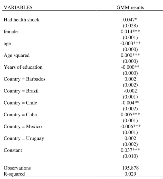
Instrumenting for Health Shocks

An issue with the previous estimates is the potential for bias due to the endogeneity of

heart attacks, cancer and strokes. Many lifestyle characteristics and demographic variables affect

onset of these illnesses, ability to work independent of the occurrence of a particular shock, and

employment opportunities. To attempt to correct for the endogeneity of health shocks, I

employed the instrumental variables technique, using various childhood environmental and

health conditions to predict the probability of a health shock occurring at each age. The

two-stage linear probability regression I used took the form

(2) ℎ𝑒𝑎𝑙𝑡ℎ𝑠ℎ𝑜𝑐𝑘_𝑖,𝑡 = 𝛼₁𝑎𝑔𝑒_𝑖 + 𝛼₂𝑐ℎ𝑙𝑑. 𝑤𝑒𝑎𝑙𝑡ℎ_𝑖+ 𝛼₃𝑐ℎ𝑙𝑑. ℎ𝑒𝑎𝑙𝑡ℎ_𝑖 + 𝛼₄𝑐ℎ𝑙𝑑. ℎ𝑢𝑛𝑔𝑒𝑟_𝑖 +

𝛼15𝑍𝑖 + 𝜀𝑖

(3) 𝑅_𝑖,𝑡 = 𝛽𝑋_𝑖,𝑡+ 𝛼₁𝑐𝑜𝑢𝑛𝑡𝑟𝑦_𝑖 + 𝛼₂ℎ𝑒𝑎𝑙𝑡ℎ𝑠ℎ𝑜𝑐𝑘_𝑖,𝑡 + 𝜀_𝑖,𝑡

In (2), 𝑐ℎ𝑙𝑑. 𝑤𝑒𝑎𝑙𝑡ℎ𝑖 is a categorical variable indicating whether the respondent’s

family’s economic situation was good, average, or poor during the respondent’s first 15 years of

life. Similarly, 𝑐ℎ𝑙𝑑. ℎ𝑒𝑎𝑙𝑡ℎ_𝑖 is a categorical assessment of the respondent’s childhood health

and 𝑐ℎ𝑙𝑑. ℎ𝑢𝑛𝑔𝑒𝑟𝑖 is a dummy variable indicating whether or not the respondent experienced

hunger as a child. 𝑍_𝑖 is a vector of dummy variables indicating whether or not the respondent

suffered from health conditions or illnesses including measles, bronchitis, kidney disease,

(18)

describing a causal relationship between health shocks and retirement, I make the assumption

that these childhood variables are independent of factors influencing future employment aside

from their effect on likelihood of experiencing a health shock.

In the second stage regression, given by equation (3), 𝑋_𝑖,𝑡 is, as before, a vector of

time-variant individual characteristics. For this regression I excluded both measurements of health

status—self-reported and objective—as well as whether or not the respondent smokes as these

are endogenous as well. Tab1e 6 reports the results of the second stage equation. Post estimation

tests indicate that my instrument is valid. My first stage regression has an F statistic of 0.000,

indicating a strong instrument and the model is not overidentified. The test of endogeneity failed

to reject the null hypothesis that health shocks are endogenous. However, the test has been

demonstrated to perform poorly when the variable being instrumented is binary.17

I find that health shocks could have a much larger effect that my initial estimates

suggested. A health shock increases the hazard of retirement by 4.7%, an effect over twice as

large as the marginal effect of 1.8% calculated in my base regression. However, since I have

omitted other measurements of health from this regression due to their likely endogeneity, health

shocks in this regression encompass all health-related information and this likely explains some

of the reason for the large increase in importance. Consistent throughout, however, is the

conclusion that serious health conditions exert strong influences on the timing of retirement. The

instrumental variables regression also indicates that country of residence has a significant impact

on the timing of workforce exit.

(19)

VI. Conclusion

Among the variables examined in this paper, health shocks in the form of heart attacks,

strokes, and cancer are prominent in terms of impact on workforce exit. The effect of these

shocks seems to vary somewhat across educational groups and gender, but largely affect people

in the seven Latin American countries sampled similarly, regardless of the country of residence

or pension scheme differences. It would be interesting to compare the effects health shocks

across more diverse countries with stronger and weaker welfare systems to determine whether or

not this relationship holds outside of South America. With only data from these South American

and Caribbean countries, however, I am unable to conclude that social security schemes have a

significant impact on how people respond to health shocks.

Measurable health variables such as health shocks however, are not the only factor that

can influence the timing of retirement. My data suggests that self-assessed health is a stronger

predictor of retirement than is the objective composite measure that was available.

Non-measurable components of health and perceived health are important as well.

Differences across countries appear to affect the age at which people retire in the absence

of a health shock. Interestingly given Brazil’s budgetary problems resulting from long

retirements during which people draw on generous pensions, Brazilians had a lower hazard of

retiring when health status, health shocks, and other factors were controlled for than did any of

the countries except Chile. From this data, we cannot determine whether these cross-country

differences are due to cultural norms, population health, social security policies, or other factors.

However, economic theory and the literature indicate that social security generosity does affect

retirement decisions and my analysis suggests that at least some of the social security reforms

(20)

reforms tended to increase the retirement hazard, thereby reducing the average age of retirement.

This result suggests that the reforms may have been a boon to older workers who wanted to retire

(21)

Bibliography

Aguila, Emma. “Male Labor Force Participation and Social Security in Mexico.” Journal of

Pension Economics and Finance Vol. 3, Issue 2: 145-171 (2014).

Atlas, Steven J. and Jonathan S. Skinner. “Education and the Prevalence of Pain.” National

Bureau of Economic Research (May 2009), Accessed October 17, 2015. doi: 10.3386/w14964

Barrientos, Armando. “Work, Retirement, and Vulnerability of Older Persons in Latin America:

What are the Lessons for Pension Design?” Journal of International Development (May

2000), 12: 495-506 (2000).

Benitez-Silva, Hugo, Moshe Buchinshy, Hiu Man Chan, Sofia Cheidvasser, and John Rust.

“How Large is the Bias in Self-Reported Disability?” Journal of Applied Econometrics

19: 649-670 (2004).

Bound, John. “Self-Reported versus Objective Measures of Health in Retirement Models.” The

Journal of Human Resources Vol. 26, No. 1: 106-138 (1991).

Case, Anne and Angus Deaton. “Broken Down by Work and Sex: How Our Health Declines.”

Analyses in the Economics of Aging (2005).

Cooper, Richard S., Joan F Kennelly, and Pedro Orduñex-Garcia. “Health in Cuba.”

International Journal of Epidemiology Vol. 35, Issue 4: 817-824 (2006). Eibich, Peter. “Understanding the Effect of Retirement on Health.” Journal of Health

Economics, Vol. 43: 1-12 (2015).

(22)

Gendell, Murray. “Retirement Age Declines Again in 1990s.” Monthly Labor Review, October

2001.

Grossman, Michael. “On the Concept of Health Capital and the Demand for Health,” Journal of

Political Economy, Vol. 80, No. 2: 223-255 (1972).

Guilkey, David K., and Peter M. Lance. “Program Impact Estimation with Binary Outcome

Variables: Monte Carlo Results for Alternative Estimators and Empirical Examples.” In

Festschrift in Honor of Peter Schmidt: Econonometric Methods and Applications, Edited by Robin Sickles and William Horrace, 5-46. New York: Springer, 2014.

Gupta, Nabanita D., and Mona Larsen. “The Impact of Health on Individual Retirement Plans:

Self-Reported Versus Diagnostic Measures.” Health Economics, Vol. 19: 792-813 (2010).

Kuhn, Michael, Stefan Wrzaczek, Alexia Prskawetz, and Gustav Feichtinger. “Optimal Choice

of Health and Retirement in a Life-Cycle Model.” Journal of Economic Theory 158: 186-212 (2015).

Laun, Tobias and Johanna Wallenius. “A Life Cycle Model of Health and Retirement: The case

of Swedish Pension Reform.” Journal of Public Economics 127: 127-136 (2015). McEniry, Mary. “Research on Early Live and Aging Trends and Effects (RELATE): A

Cross-National Study.” Ann Arbor, MI: Inter-university Consortium for Political and Social

Research [distributor], May 7, 2015. http://doi.org/10.3886/ICPSR34241 .v2

Mitchell, Olivia S. and Gary S. Fields. “The Economics of Retirement Behavior.” Journal of

(23)

Pelaez, Martha, Alberto Palloni, Cecilia Albala, Juan C. Alfonso, Roberto Ham-Chande, Anselm

Hennis, Maria Lucia Lebrao, Esther Lesn-Diaz, Edith Pantelides, and Omar Prats.

“SABE - SURVEY ON HEALTH, WELL-BEING, AND AGING IN LATIN AMERICA

AND THE CARIBBEAN, 2000 [Computer file].” ICPSR version. Washington, D.C.:

Pan American Health Organization/World Health Organization (PAHO/WHO)

[producers], 2004. Ann Arbor, MI: Inter-university Consortium for Political and Social

Research [distributor], 2005.

Riffkin, Rebecca. “Average US Retirement Age Rises to 62.” Gallup, last modified April 28,

2014. Accessed December 2, 2015.

http://www.gallup.com/poll/168707/average-retirement-age-rises.aspx

Riphahn, Regina. “Disability Retirement and Unemployment—Substitute Pathways for Labour

Force Exit? An Empirical Test for the Case of Germany.” Applied Economics 29 (5):

551-561 (1997).

Romero, Simon. “An Exploding Pension Crisis Feeds Brazil’s Political Turmoil.” The New York

Times, October 20, 2015. Accessed December 1, 2015.

http://www.nytimes.com/2015/10/21/world/americas/brazil-pension-crisis-mounts-as-more-retire-earlier-then-pass-benefits-on.html

van Erp, Frank, Niels Vermeer, and Daniel van Vuuren. “Non-financial Determinants of

Retirement: A Literature Review.” De Economist 162 (2): 167-191 (2014).

Waidmann, Timothy, John Bound, and Michael Schoenbaum. “The Illusion of Failure: Trends in

(24)

Appendix

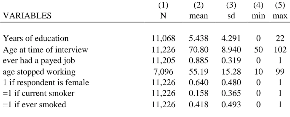
Table 1: Summary Statistics

(1) (2) (3) (4) (5)

VARIABLES N mean sd min max

Years of education 11,068 5.438 4.291 0 22

Age at time of interview 11,226 70.80 8.940 50 102

ever had a payed job 11,205 0.885 0.319 0 1

age stopped working 7,096 55.19 15.28 10 99

1 if respondent is female 11,226 0.640 0.480 0 1

=1 if current smoker 11,226 0.158 0.365 0 1

=1 if ever smoked 11,226 0.418 0.493 0 1

Notes: Summary of all observations in original data set. Age stopped working has fewer

(25)

Table 2: Base Logit Regression and Marginal Effects

VARIABLES dy/dx Logit coefficients

Had health shock 0.018*** 0.733***

(0.002) (0.074)

Time (N of years) since health shock -0.001*** -0.031***

(0.000) (0.006)

female 0.013*** 0.538***

(0.001) (0.034)

age 0.002*** 0.093***

(0.000) (0.001)

Years of education 0.000 0.003

(0.000) (0.004)

Composite health score -0.000** -0.001**

(0.000) (0.001)

Self-reported health status = fair -0.002 -0.079

(0.001) (0.048)

Self-reported health status = good -0.008*** -0.322***

(0.001) (0.051)

Self-reported health status = very good -0.008*** -0.297***

(0.002) (0.073)

Self-reported health status = excellent -0.010*** -0.413***

(0.002) (0.093)

Country = Brazil -0.004*** -0.142***

(0.001) (0.048)

Country = Chile -0.006*** -0.235***

(0.001) (0.058)

Country = Cuba 0.003** 0.123**

(0.001) (0.050)

Country = Mexico -0.010*** -0.450***

(0.001) (0.060)

Country = Uruguay 0.003* 0.093*

(0.001) (0.049)

ever smoked 0.000 0.009

(0.001) (0.034)

Constant -8.663***

(0.101)

Observations 190,948 190,948

Standard errors in parentheses *** p<0.01, ** p<0.05, * p<0.1

(26)

Table 3: Regression with Policy Variables

(0.002) (0.075)

(0.000) (0.006)

female 0.014*** 0.560***

(0.001) (0.028)

age 0.002*** 0.092***

(0.000) (0.001)

Years of education 0.000 0.001

(0.000) (0.003)

Self-reported health status = fair -0.003** -0.108**

(0.001) (0.046)

(0.001) (0.048)

(0.002) (0.067)

(0.002) (0.087)

Country = Barbados 0.012

(0.064)

Country = Brazil -0.123*

(0.065)

Country = Chile -0.005** -0.173*

(0.002) (0.100)

Country = Cuba 0.139**

(0.064)

Country = Mexico -0.008*** -0.384***

(0.001) (0.074)

Country = Uruguay 0.003* 0.024

(0.002) (0.067)

Switched to individual retirement accounts 0.009*** 0.362***

(0.003) (0.126)

Years since implementation of individual accounts 0.000 0.008

(0.000) (0.010)

Argentina # pen_reform -0.379***

(0.130)

Chile # pen_reform -0.588***

(0.155)

Mexico # pen_reform -0.336**

(0.136)

Uruguay # pen_reform 0.000

(27)

hlt_hadshock # pen_reform 0.111 (0.107)

(28)

Table 4: Education and Gender Interactions

(0.005) (0.203)

(0.000) (0.006)

1 if respondent is female 0.010*** 0.380***

(0.002) (0.093)

age 0.002*** 0.097***

(0.000) (0.001)

Educational category: Some secondary -0.001 -0.046

(0.001) (0.050)

Educational category: Some college -0.005*** -0.247***

(0.001) (0.068)

Educational category: College + -0.009*** -0.359***

(0.001) (0.081)

(0.001) (0.052)

(0.001) (0.053)

(0.002) (0.072)

(0.002) (0.091)

(0.001) (0.034)

Type of work: intellectual 0.012*** 0.415***

(0.001) (0.044)

Type of work: mixed -0.001 -0.033

(0.001) (0.044)

Country = Barbados -0.001 -0.045

(0.001) (0.057)

Country = Brazil -0.005*** -0.195***

(0.001) (0.055)

Country = Chile -0.005*** -0.201***

(0.002) (0.066)

Country = Cuba 0.002 0.081

(0.002) (0.057)

Country = Uruguay 0.001 0.047

(0.002) (0.057)

hlt_hadshock # education = primary 0.276

(0.202)

(29)

(0.226)

hlt_hadshock # education = some college 0.413*

(0.241)

hlt_hadshock # education = college + 0.000

(0.000)

hlt_hadshock # female 0.212**

(0.097)

Constant -9.059***

(0.105)

(30)

Table 5: Country Interactions and Marginal Effects

(0.003) (0.116)

(0.000) (0.006)

female 0.014*** 0.570***

(0.001) (0.033)

age 0.002*** 0.097***

(0.000) (0.001)

Years of education -0.000*** -0.019***

(0.000) (0.004)

(0.001) (0.052)

(0.001) (0.054)

(0.002) (0.072)

(0.002) (0.092)

Country = Barbados -0.001 -0.065

(0.002) (0.060)

Country = Brazil -0.006*** -0.229***

(0.001) (0.060)

Country = Chile -0.006*** -0.231***

(0.002) (0.071)

Country = Cuba 0.002 0.056

(0.002) (0.060)

Country = Uruguay 0.001 0.008

(0.002) (0.061)

hlt_hadshock # Argentina -0.201

(0.180)

hlt_hadshock # Barbados 0.073

(0.182)

hlt_hadshock # Brazil -0.181

(0.142)

hlt_hadshock # Chile -0.163

(0.169)

hlt_hadshock # Cuba 0.067

(0.145)

hlt_hadshock # Mexico 0.000

(0.000)

Work type = intellectual 0.012*** 0.407***

(31)

Work type = mixed -0.000 -0.017

(0.001) (0.044)

(0.001) (0.034)

Constant -8.944***

(0.107)

(32)

Table 6: Instrumenting for Health Shocks

VARIABLES GMM results

Had health shock 0.047*

(0.028)

female 0.014***

(0.001)

age -0.003***

(0.000)

Age squared 0.000***

(0.000)

Years of education -0.000**

(0.000)

Country = Barbados 0.002

(0.002)

Country = Brazil -0.002

(0.001)

Country = Chile -0.004**

(0.002)

Country = Cuba 0.005***

(0.001)

Country = Mexico -0.006***

(0.001)

Country = Uruguay 0.002

(0.002)

Constant 0.037***

(0.010)

Observations 195,878

R-squared 0.029

Robust standard errors in parentheses *** p<0.01, ** p<0.05, * p<0.1

(33)

Figure 1: Retirement Age by Country

Notes: Middle quartiles and median retirement age for each country are denoted by the vertical rectangles and the lines dividing the rectangles, respectively. Points represent outliers.

0

20

40

60

80

1

0

a

g

e

st

o

p

e

d

w

o

rki

n

g

(34)

Figure 2: Workforce Survival Hazard by Gender

Notes: Lines indicate the likelihood of an individual remaining in the workforce at each age. Probability of remaining in the workforce is 1 before the age of 35 as I have excluded individuals retiring before that age from my estimation sample.

0

.2

5

.5

.7

5

1

0 5 10 15 20 25 30 35 40 45 50 55 60 65 70 75 80 85 90 95 100

analysis time

95% CI 95% CI

gender = Male gender = Female

(35)

Figure 3

Notes: Sample is respondents from Brazil, Cuba, and Mexico. Lines indicate the probability of remaining in the workforce at each age. As in figure 2, individuals who left the workforce before the age of 35 are excluded.

0

.2

5

.5

.7

5

1

0 5 10 15 20 25 30 35 40 45 50 55 60 65 70 75 80 85 90 95 100

analysis time

95% CI 95% CI 95% CI

Brazil Cuba Mexico

(36)

Figure 4

Notes: Lines indicate the likelihood of an individual remaining in the workforce at each age. Probability of remaining in the workforce is 1 before the age of 35 as I have excluded individuals retiring before that age from my estimation sample.

0

.2

5

.5

.7

5

1

0 5 10 15 20 25 30 35 40 45 50 55 60 65 70 75 80 85 90 95 100

analysis time

95% CI 95% CI

edu_cat = Less than primary edu_cat = College +