Sharif University of Technology
Scientia IranicaTransactions B: Mechanical Engineering http://scientiairanica.sharif.edu
Using an optimized RBF neural network to predict the
out-of-plane welding distortions based on the 3-2-1
locating scheme
M.M. Tafarroj and F. Kolahan
Department of Mechanical Engineering, Ferdowsi University of Mashhad, Mashhad, Iran. Received 28 October 2017; received in revised form 12 December 2017; accepted 8 January 2018
KEYWORDS GTAW; Distortion;
3-2-1 locating scheme; RBF;
Optimization; Simulated annealing.
Abstract. This study deals with the eect of locator positioning in the 3-2-1 locating scheme to control the out-of-plane distortion in gas tungsten arc welding of sheet metals. To apply this locating scheme to the sheet metals, a suitable xture was designed. The distortion of the welded plates was predicted using the Radial Basis Function (RBF) neural network. To gather the experimental data employed in the RBF modeling process, a set of welding tests was performed on the sheet specimens by varying the positions of the three locators. The parameters of the network were optimally selected using the Simulated Annealing (SA) optimization algorithm. The average and maximum errors computed for the test dataset were respectively 2.43% and 5.30% while in some cases, the error fell below 1%. The results of the RBF network showed very good agreement with the experiments and it can be concluded that this modeling technique can be utilized successfully in predicting the welding distortions when the 3-2-1 locating scheme is used.
© 2019 Sharif University of Technology. All rights reserved.
1. Introduction
Welding is one of the most well-known methods to join materials permanently. Roughly speaking, welding of machinery parts is inevitable for most of the engineer-ing requests [1]. Selectengineer-ing the weldengineer-ing process type is contingent on the structure, technical requirements, and application conditions [2]. As a class of fusion welds, the Gas Tungsten Arc Welding (GTAW), also known as the Tungsten Inert Gas (TIG) welding process, is widely used for joining thin sheet metals remarkably implemented in aerospace, naval, and au-tomobile industries. This type of welds is performed by the use of a non-consumable tungsten electrode together with inert shielding gas, like argon, which
*. Corresponding author.
E-mail address: [email protected] (F. Kolahan) doi: 10.24200/sci.2018.5458.1282
protects the weld from atmospheric contamination [3]. However, extremely non-uniform heating during the welding process causes distortion, especially in thin structures, since the weldment heats and cools. The welding distortions will lead to many problems like loss of dimensional control and structural integrity, diculty in subsequent alignment with the adjacent component, and increase in fabrication costs with straightening [4].
As shown in Figure 1, welding distortions can be classied into six dierent types including transverse shrinkage, longitudinal shrinkage, and rotational dis-tortion, which are known as the in-plane distortions, and the angular distortion, bending distortion, and buckling, which are the out-of-plane distortions [4-6]. It should be noted that multiple types of these distortions may occur at the same time in welded structures and it is sometimes dicult to distinguish the types of distortion present in a workpiece [5].
distor-Figure 1. Various types of welding distortions [5].
tions. Thus, it is dicult to control this phenomenon by only relying on practical experiences. If distortions can be forecasted before welding, mitigating of this unwanted event can be done successfully [7].
Many studies have been done to predict and control the welding induced distortions. Thanks to the development of high-speed computers, the Finite Element Analysis (FEA) can be used to simulate and predict the welding distortions. Pazooki et al. [5] conducted a study to control the gas metal arc welding distortions by the use of additional heat source. In addition to the experiments, they used a 3D nite element model to understand the distortion reduction mechanism. Deng et al. [7] investigated the eect of external restraint on the welding deformations. In their research, six clamps were employed to restrain the welded specimens. Both numerical results and exper-iments proved that external restraint could mitigate the nal deformation to some extent. Li et al. [8] investigated the eect of welding parameters on the weld shape and distortion of the Ti2AlNb alloy joint. The eect of xtures on the welding distortion was also studied, and it was shown that welding without xtures in bead-on-plate welding would cause less distortion than the butt welds.
Compared to their many capabilities in modeling of various processes, the applications of Articial Neu-ral Networks (ANNs) in predicting the welding induced distortion are still rare. Therefore, the implementation of ANNs and meta-heuristic optimization algorithms is a promising and exciting area of welding researches. Lightfoot et al. [9] established an ANN model to predict the welding distortion of the steel plates. They also performed a sensitivity analysis to nd out the factors aecting the welding distortion. Bruce and Lightfoot [10] modeled the distortion caused by welding operation using the ANN and found that the results of the ANN well tted the actual values. Yang and Shao [11] developed a thermo-mechanical model to forecast the welding residual stress and distortion. In this research, the welding sequence causing the minimum distortion was determined using the Genetic Algorithm (GA), and at last, the optimization strategy
was successfully pursued for a real product. Choobi et al. [12] used an ANN structure to forecast the angular distortions in single-pass butt-welded 304 stainless steel plates. They employed a set of FEM results obtained for various plate dimensions as the ANN inputs. Barclay et al. [13] investigated the suitability of the induction heating process with the traveling induction coil to rectify the welding angular distortion. By using the experimental data, they considered an ANN to predict the distortion. According to their ndings, the ANN was well-suited to predict the nal distortion of the plate for both after-welding and induction heating. Tian et al. [14] developed a back-propagation neural network to predict the transverse shrinkage and angular distortion in bead-on-plate GTA welding of S304L stainless steel. The employed data to construct the neural network were captured from the FEM simulation while the accuracy of numerical results was veried by the experiments. The same work has also been performed by Narayanareddy et al. [15].
As it can be seen, several studies have been con-ducted on the welding distortions. However, the work on the eect of jigs and xtures on the welding induced distortions is relatively rare [7,8,16-18]. Therefore, the eect of jigs and xture as the external mechanical constraints aecting the welding distortions can be further attended to. In addition, a thorough search through the relevant literature on the application of 3-2-1 locating scheme in arc welding operations yielded very limited works [19].
This paper focuses on the application of 3-2-1 locating scheme in GTAW process for sheet metals with regards to the resultant distortion in the workpiece. The main purpose is to evaluate the out-of-plane dis-tortion, as aected by various arrangements of locators. To achieve this, an Articial Neural Network (ANN) model is developed for accurately predicting the nal distortion of the welded workpiece when the positions of locators are simultaneously changed.
The study is organized as follows: in Section 2, the 3-2-1 locating scheme is introduced. In Section 3, the tools used in this work, the Radial Basis Function (RBF) neural network, and the Simulated Annealing
(SA) optimization technique are briey presented. Sec-tion 4 explains the procedure for the experimental work, including experiment setups and output mea-surements. The main ndings of this research are presented and discussed in Section 5. Finally, the concluding remarks are rendered in Section 6.
2. The 3-2-1 locating scheme
The 3-2-1 locating scheme is a method utilized to re-strain all 6 (Degree of Freedom) DoFs2of a workpiece.
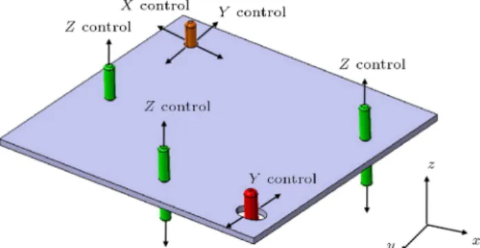
According to Figure 2, the points A1, A2, and A3 construct a plane and restrain the translation in z-direction and rotation in x- and y-z-directions. Addition-ally, the points B1 and B2 dene a line and restrain the translation in y-direction and rotation in z-direction. Finally, C1 locks the translation in x-direction. An adequately designed xture for sheet metals usually needs N 3 carefully selected locators on the primary datum plane to restrain deformation of the part [20].
In 3-2-1 locating approach, the 2-1 locating is applied by using a 4-way pin and a 2-way pin. A typical illustration of the 3-2-1 locating scheme is provided in Figure 3. As can be seen, the 4-way and 2-way pins restrain the translations in x- and y-directions and
Figure 2. The 3-2-1 locating scheme.
Figure 3. A typical 3-2-1 locating scheme applied to a plate.
rotation in z-direction.
For any arrangement of locators constraining the z-direction and the rotations in x- and y-directions, if a method is presented to predict the distortion prior to the welding operation, considerable values of time and cost can be saved.
3. Modeling approach
3.1. The Radial Basis Function (RBF) network
An articial neural network is a processing system of information initially inspired by the biological neural units. ANNs method can be a noteworthy tool for material design. It is common to regard an ANN as a \black box" concentrated on the prediction accu-racy [21].
The radial basis functions are neural networks with three xed layers. Simple structure of such networks has the advantage of lower processing time. The ability of online learning, high power of extending the results and generalization, and high tolerance to input noises are the other advantages of the RBF networks [22]. Thanks to the high capability of generalization, the RBFs are suitable techniques to gure out the patterns not used in training procedure. RBF networks have robust tolerance to the input noise, which improves the stability of the constituted systems. Therefore, it is sensible to consider RBF as a competitive approach to modeling of nonlinear problems [23]. As stated previously, an RBF has three layers. The numbers of input and output neurons are imposed by the problem at hand. The Gaussian functions are implemented in the hidden layer while the sigmoid or linear functions are used in the output layer. A schematic view of the constructed RBF is illustrated in Figure 4. In the gure, inputs are the positions of the locators represented by Pi and the output is the
welding induced distortion.
In the RBF, the goal is to dene a function like f( ~X) shown in Eq. (1).
f( ~Xp) = tp 8p = 1; 2; :::; P; (1)
where ~Xp is the pattern number p and tp is its
corresponding desired value. This can be done by mapping the D-dimensional input vectors ~Xp = fXp
i :
i = 1; :::; Dg onto the output tp. The RBF denes m1
P basis functions based on the form ~X X~p
where is a nonlinear function. Therefore, the output function can be generally formulated via Eq. (2).
f( ~X) =XP
p=1
wp ~X X~p
: (2)
Now, the problem is to nd the weights wp such that
the function can be tted to the data. Combining both Eqs. (1) and (2) yields Eq. (3), which is useful to evaluate the weights:
f( ~Xq) =XP p=1
wp ~Xq X~p
= tq: (3)
Introducing the matrix notations t = ftpg, w = fw pg,
and = fpq = ( ~Xq X~p), Eq. (3) can be
written as Eq. (4):
w = t: (4)
Now, having the inverse of matrix , one can simply attain the weight matrix via Eq. (5).
w = 1t: (5)
When the weights are available, a function f( ~X) exists that can be tted to the point data. The most common basis function is Gaussian function (Eq. (6)):
(r) = exp
r2
22
( > 0): (6)
In Eq. (6), the value of is known as the spread. To achieve the best performance of the RBF network, this parameter together with the maximum number of neurons added to the hidden layer must be carefully determined. Thus, an optimization procedure using the Simulated Annealing (SA) algorithm is utilized in the following for optimal determining of these parameters. 3.2. RBF optimization procedure
The RBF is employed to predict the welding induced distortion. To get the best performance of the RBF, its parameters should be optimally selected. Therefore, the simulated annealing optimization algorithm is em-ployed to determine the best combination for the values of the RBF parameters.
Determining the best combination of variables which yields the best process performance is the goal of
an optimization process [24]. Simulated annealing is an optimization algorithm rst introduced by Kirkpatrick et al. to solve hard optimization problems [25]. It was inspired by the process of physical annealing of solids. In the annealing process, a solid is heated to a high temperature until all molecules can move freely. Annealing (slow cooling) would result in a perfect crystalline in which all atoms are arranged in low-level energy lattice.
In the SA algorithm, slow cooling of the metallur-gical annealing is simulated by the parameter T and the rate of its reduction (called cooling schedule). Starting from a high temperature and slowly reducing it, to some extent, prevents being trapped in local optima.
Therefore, in early iterations, the value of T should be high enough to make sure of escaping from local optima. In the beginning, when T is high, non-improving solutions are more likely to be accepted. When the algorithm proceeds, the value of temperature is gradually reduced and, hence, only the improving solutions are accepted.
The main idea of this technique is to generate a random solution. Then, a new solution is created in the neighborhood of the current solution. If the new point is better, it is accepted; but if it is worse, the new solution can be accepted or rejected based on probability. For minimizing an objective, the pseudocode of the SA algorithm can be written as:
1. Select a random initial point ~X0, call the RBF, and
evaluate the objective function f( ~X0);
2. Generate a new point ~X in the neighborhood of ~X0,
call the RBF, and evaluate the objective function f( ~X);
3. Calculate f = f( ~X) f( ~X0) and p = e Tf;
4. If f < 0, set ~X0= ~X and go to step 5. Otherwise,
generate a random number 2 (0 1); if < p, set ~
X0= ~X and go to step 5. Else, go to step 2;
5. Reduce the value of T by some linear or logarithmic approach (for example, T = kT where 0 < k < 1);
6. If the stopping criterion of the algorithm is not sat-ised, go to step 2 as the next iteration; otherwise, go to step 6;
7. Stop the algorithm and present the optimal point. At each iteration, to generate a new solution vector ( ~X) in step 2 of the SA algorithm, an element of the current solution vector ( ~X0) is selected randomly.
Then, the element is changed to a random value within its permitted range. For example, assume that X0 = (0:11; 4) and the rst element of ~X0 (i.e. 0.11)
is randomly selected to change. It is supposed that the permitted range of the selected element is [0.1,10]. Therefore, a random value is generated in this range
(e.g. 0.80). Now, the new generated neighbor solution to be evaluated is ~X = (0:80; 4).
The two main parameters of the RBF which should be optimally tuned are the spread (Sp) and the maximum number of neurons (N). The objective function of the problem can be stated by Eq. (7):
min f( ~X) = MRE( ~X) + abs(1=Cr); 0:1 Sp 10;
1 N 15: (7)
In Eq. (7), ~X = (Sp; N) is the solution vector containing the optimization variables, the MRE is the mean relative error computed for test dataset, and Cr is the correlation coecient between the target values (values obtained from the experiments) and the network outputs computed for the test dataset. After the process of determining the optimum values of the RBF parameters, the results of the optimized RBF will be presented.
4. Experimental procedure 4.1. Materials and equipment
An air-cooled PSQ 250 AC/DC (GAAM ELECTRIC-Co, Iran) semi-automatic welding machine with 250 ampere capacity and high pulse frequency (up to 500 Hz) was used to perform experiments on the St12 steel sheets. The relative motion between the weldments and the torch was carried out using an automatic table with controllable linear motion. A new xture was designed, which was suitably able to apply the N-2-1 locating scheme. When the plate is placed between the upper and lower parts of the xture, the locators x the plate in z-direction, which is normal to the plate, and avoid the rotation in x- and y-directions. The welding machine, automated table, the GTAW air-cooled torch with ceramic nozzle, and the designed xture are exhibited in Figure 5.
Because of good welding performance and rela-tively high dimensional accuracy, the St12 steel has widely been employed to manufacture various automo-tive parts. The chemical composition and mechanical properties of St12 steels are respectively presented in Tables 1 and 2. The shielding gas was pure argon and because the plate was thin, the welding was done without any ller metal.
Table 1. Chemical composition of St12 steel (wt%).
Element C Mn P S
Amount 0.12 0.6 0.045 0.04
Figure 5. The equipment used in experiments: (a) The PSQ 250 AC/DC welding machine, (b) the table with controllable linear motion, and (c) the welding torch and the designed xture.
Figure 6. The predetermined sub-regions in which the locators could move.
Table 2. Mechanical properties of St12 steel. Property Tensile
strength
Yield strength
Total elongation Value 270-410 MPa 140-280 MPa 28%
4.2. Welding experiments and measurements After setting up the required equipment, the specimens were welded together. Since the independent variables were the locations of three locators, as can be seen in Figure 6, the plate region was divided into three sub-regions and the locators could be moved to some
Table 3. The values of welding parameters.
Parameter Current (I) Voltage (V) Speed (S) Torch height (h) Gas ow rate (Q)
Value 100 A 14 V 160 mm/min 2 mm 8 L/min
Figure 7. The method of distortion measuring.
Figure 8. A sample of the welded plates.
predetermined locations.Thus, as can be seen in Figure 6, each design variable had four levels.
The other welding parameters (current, voltage, speed, gas ow rate, torch height with respect to the plate surface) shown in Table 3 were constant during the welding operation.
Before welding, three points on the plate were marked to measure the welding distortion. After welding, the displacement of the three points with respect to the surface underneath was measured using a simple method, which is illustrated in Figure 7. Then, the obtained values were averaged and the distortion value of the welded plate was recorded.
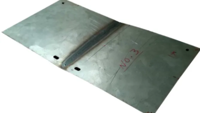
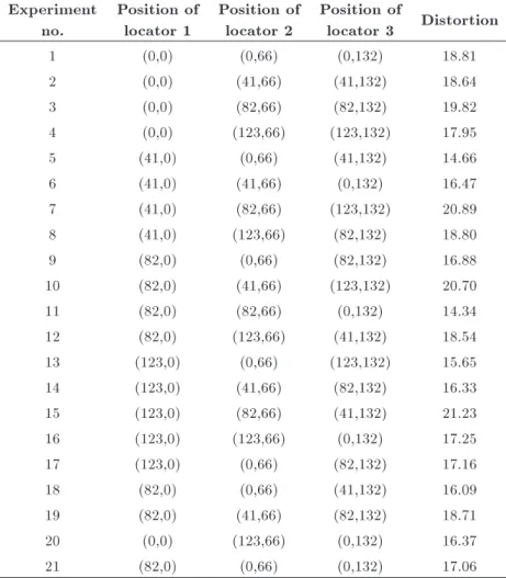
Based on the design assumption, 21 experiments were conducted. The locators' (x; y) coordinates along with their resultant distortion are reported in Table 4. A sample of the welded plates is demonstrated in Figure 8.
The procedure for conducting the welding exper-iments, when the 3-2-1 locating scheme is applied to control the welding distortion, is very time consuming and expensive. Thus, it is necessary to introduce a novel approach to predict the welding induced distor-tion when the 3-2-1 locating scheme is applied. In
the next section, an RBF articial neural network is constructed to solve the problem.
5. Results and discussion
The experimental data were employed to train an RBF model. For this purpose, each predetermined position of locators shown in Figure 6 was coded by a number. For instance, in region 1, the rst, second, third, and fourth locations were respectively coded by 1, 2, 3, and 4. This coding method was also used for the other two regions. With this coding method, the rst experiment had the inputs (1, 1, 1) and so on. Among all data reported in Table 4, six data were set o from the rest as the test data, which were not used in the training process. These data were presented to the network after nishing the network training to examine the network capability in predicting new data. The other 15 data were employed as the training data.
The algorithm was written using MATLAB R2014b and run for 5000 iterations. The range of Sp was selected to be between [0.1,10] with the step of 10 2. Likewise, N was set to vary between [1,15] with
the step of 1. The convergence plot of the SA algorithm is illustrated in Figure 9.
It can be seen that due to the random nature of the SA, in the early iterations, the objective function values are very large. Furthermore, the behavior of the objective function values is strongly oscillating, and it cannot be condently concluded that the best answer has been found. The minimum value of the objective
Figure 9. The SA convergence procedure for optimizing the RBF parameters.
Table 4. The performed experiments (dimensions are in millimeter). Experiment
no.
Position of locator 1
Position of locator 2
Position of
locator 3 Distortion
1 (0,0) (0,66) (0,132) 18.81
2 (0,0) (41,66) (41,132) 18.64
3 (0,0) (82,66) (82,132) 19.82
4 (0,0) (123,66) (123,132) 17.95
5 (41,0) (0,66) (41,132) 14.66
6 (41,0) (41,66) (0,132) 16.47
7 (41,0) (82,66) (123,132) 20.89
8 (41,0) (123,66) (82,132) 18.80
9 (82,0) (0,66) (82,132) 16.88
10 (82,0) (41,66) (123,132) 20.70
11 (82,0) (82,66) (0,132) 14.34
12 (82,0) (123,66) (41,132) 18.54
13 (123,0) (0,66) (123,132) 15.65
14 (123,0) (41,66) (82,132) 16.33
15 (123,0) (82,66) (41,132) 21.23
16 (123,0) (123,66) (0,132) 17.25
17 (123,0) (0,66) (82,132) 17.16
18 (82,0) (0,66) (41,132) 16.09
19 (82,0) (41,66) (82,132) 18.71
20 (0,0) (123,66) (0,132) 16.37
21 (82,0) (0,66) (0,132) 17.06
function is 1.065 and it occurs at ~X = (0:86; 9). By considering the computational cost, the number of iterations is set to 5000. It is clear that approximately after 3500 iterations, no improvement can be observed in the objective function value; but, to ensure that the algorithm will converge on the optimum value, more iterations are needed. To better realize the behavior of the objective function, it is noteworthy to check the standard deviation of the objective function for every 200 iterations (see Figure 10). The function shown in Figure 10 is a decreasing function. It can be seen that, in the initial iterations, the standard deviations are high. When the number of iterations increases, the standard deviation of the objective function decreases. In the nal iterations, the standard deviation of the objective function approximately tends to zero. This is because the algorithm converges on the optimum point.
The optimal parameters obtained from the SA lead to nding the best outcomes for the radial basis function network. Using the attained RBF parameters, the network outputs against the targets and the corre-lation plot for the train data are presented in Figures 11
and 12, respectively. The gures show that the training procedure has successfully been performed.
Now, to examine the performance of the network against the data not used in the training, the test dataset is presented to the trained network.
The relative error, which is hereafter briey called
Figure 10. The standard deviation of the objective function for every 200 iterations.
Figure 11. Predicted outputs versus the targets for the train dataset.
Figure 12. The correlation between the predicted values by the RBF and the targets for the train data.
the error, is a suitable criterion to evaluate the per-formance of an ANN. It is computed via Eq. (8). In Eq. (8), T and O are respectively the targets and the network outputs.
RE = jT TOj 100: (8)
The network outputs versus the targets and the plot of correlation between the targets and the network output have been illustrated in Figures 13 and 14, respectively. The gures prove that the targets and the predicted values are very close and the correlation between both datasets is high.
Furthermore, the target values, the network out-puts, and errors calculated for each of the test data have been displayed collectively in Figure 15. It can
Figure 13. Predicted outputs versus the targets for the test dataset.
Figure 14. The correlation between the predicted values by the RBF and the targets for the test data.
Figure 15. The errors calculated for the test data together with the targets and network outputs.
be seen that the relative errors are all acceptable. Especially, the maximum error (5.30%) corresponds to datum number 16 and the minimum one (0.43%) corresponds to datum number 7.
As it is shown, the optimized radial basis function has a high capability in predicting the welding induced distortion. Since the welding distortions have a high degree of nonlinearity and the process of preparing welding setup and test samples is very expensive and time consuming, proposing such an approach that can accurately model the process is very crucial.
6. Conclusion
Welding induced distortion is a very complicated and nonlinear phenomenon. Also, purely experimental approach to measure distortions under various settings is very time consuming and expensive, and it needs skillful operators. In this research, it was shown that the RBF was a powerful tool for modeling the GTAW process and predicting the resultant distortions using a limited number of experimental data. In this way, an accurate distortion prediction could be achieved under a given arrangement of the locators in 3-2-1 locating method. The experiments were conducted on the St12 steel plates widely used in automotive industry and other consumer products. To apply the 3-2-1 locating scheme to the sheet metals, a suitable xture was designed.
In the modeling process, the performance of the RBF model was further improved using the SA algorithm. The RBF outputs obtained for both the training and test datasets were very close to the actual values. The average error computed for the test dataset was 2.43% with maximum error value of 5.30% and the minimum value less than 1%. Furthermore, the correlation coecient between the targets and the outputs of the network when the test data were presented to the network was 0.9617. This shows that both sets of the data were highly correlated.
These ndings illustrate that the proposed ap-proach can eectively be employed to evaluate any given arrangement of the locators in terms of the out-of-plane distortions. In this way, the best possible arrangement of the locators may be identied and implemented. This part is an ongoing research. References
1. Ates, H., Dursun, B., and Kurt, E. \Estimation of mechanical properties of welded S355J2+ N steel via the articial neural network", Scientia Iranica Transaction B: Mechanical Engineering, 23(2), p. 609 (2016).
2. Zhang, W.W., Cong, S., Huang, Y., and Tian, Y.H. \Micro structure and mechanical properties of vacuum brazed martensitic stainless steel/tin bronze by Ag-based alloy", Journal of Materials Processing Technol-ogy, 248 (Supplement C), pp. 64-71 (2017).
3. Narang, H., Mahapatra, M., Jha, P., and Biswas, P. \Optimization and prediction of angular distortion and weldment characteristics of TIG square butt joints", Journal of Materials Engineering and Performance, 23(5), pp. 1750-1758 (2014).
4. Ma, N., Wang, J., and Okumoto, Y. \Out-of-plane welding distortion prediction and mitigation in sti-ened welded structures", The International Journal of Advanced Manufacturing Technology, 84(5-8), pp. 1371-1389 (2016).
5. Pazooki, A., Hermans, M., and Richardson, I. \Control of welding distortion during gas metal arc welding of AH36 plates by stress engineering", The International Journal of Advanced Manufacturing Technology, 88(5-8), pp. 1439-1457 (2017).
6. Michaleris, P., Minimization of Welding Distortion and Buckling: Modelling and Implementation, Micha-leris, P., Ed., 1st, Edn., pp. 3-4, Woodhead Publishing, Cambridge CB22 3HJ, UK (2011).
7. Deng, D., Liu, X., He, J., and Liang, W. \Investigating the inuence of external restraint on welding distortion in thin-plate bead-on joint by means of numerical sim-ulation and experiment", The International Journal of Advanced Manufacturing Technology, 82(5-8), pp. 1049-1062 (2016).
8. Li, Y., Zhao, Y., Li, Q., et al. \Eects of welding con-dition on weld shape and distortion in electron beam welded Ti2AlNb alloy joints", Materials & Design, 114, pp. 226-233 (2017).
9. Lightfoot, M., McPherson, N., Woods, K., and Bruce, G.D. \Articial neural networks as an aid to steel plate distortion reduction", Journal of Materials Processing Technology, 172(2), pp. 238-242 (2006).
10. Bruce, G. and Lightfoot, M. \The use of articial neu-ral networks to model distortion caused by welding", International Journal of Modelling and Simulation, 27(1), pp. 32-37 (2007).
11. Yang, H. and Shao, H. \Distortion-oriented welding path optimization based on elastic net method and genetic algorithm", Journal of Materials Processing Technology, 209(9), pp. 4407-4412 (2009).
12. Choobi, M.S., Haghpanahi, M., and Sedighi, M. \Pre-diction of welding-induced angular distortions in thin butt-welded plates using articial neural networks", Computational Materials Science, 62, pp. 152-159 (2012).
13. Barclay, C., Campbell, S., Galloway, A., and McPher-son, N. \Articial neural network prediction of weld distortion rectication using a travelling induction coil", The International Journal of Advanced Manu-facturing Technology, 68(1-4), pp. 127-140 (2013).
14. Tian, L., Luo, Y., Wang, Y., and Wu, X. \Prediction of transverse and angular distortions of gas tungsten arc bead-on-plate welding using articial neural network", Materials & Design (1980-2015), 54, pp. 458-472 (2014).
15. Narayanareddy, V., Chandrasekhar, N., Vasudevan, M., Muthukumaran, S., and Vasantharaja, P. \Nu-merical simulation and articial neural network mod-eling for predicting welding-induced distortion in butt-welded 304L stainless steel plates", Metallurgical and Materials Transactions B, 47(1), pp. 702-713 (2016).
16. Ma, N., Huang, H., and Murakawa, H. \Eect of jig constraint position and pitch on welding deformation", Journal of Materials Processing Technology, 221, pp. 154-162 (2015).
17. Choobi, M.S., Haghpanahi, M., and Sedighi, M. \In-vestigation of the eect of clamping on residual stresses and distortions in butt-welded plates", Scientia Iranica Transaction B: Mechanical Engineering, 17(5), p. 387 (2010).
18. Ma, N. and Huang, H. \Ecient simulation of welding distortion in large structures and its reduction by jig constraints", Journal of Materials Engineering and Performance, 26(11), pp. 5206-5216 (2017).
19. Lorin, S., Cromvik, C., Edelvik, F., Lindkvist, L., and Soderberg, R. \Variation simulation of welded as-semblies using a thermo-elastic nite element model", Journal of Computing and Information Science in Engineering, 14(3), p. 031003 (2014).
20. Cai, W., Hu, S.J., and Yuan, J. \Deformable sheet metal xturing: principles, algorithms, and simula-tions", Journal of Manufacturing Science and Engi-neering, 118(3), pp. 318-324 (1996).
21. Liu, G., Jia, L., Kong, B., Guan, K., and Zhang, H. \Articial neural network application to study quantitative relationship between silicide and fracture toughness of Nb-Si alloys", Materials & Design, 129, pp. 210-218 (2017).
22. Santos, R.B., Ruppb, M., Bonzi, S.J., and Filetia, A.M.F. \Comparison between multilayer feed forward neural networks and a radial basis function network to detect and locate leaks in pipelines transporting gas", Chem. Eng. Trans, 32(1375), p. e1380 (2013).
23. Yu, H., Xie, T., Paszczynski, S., and Wilamowski, B.M. \Advantages of radial basis function networks
for dynamic system design", IEEE Transactions on Industrial Electronics, 58(12), pp. 5438-5450 (2011).
24. Azadi Moghaddam, M., Golmezerji, R., and Kolahan, F. \Simultaneous optimization of joint edge geometry and process parameters in gas metal arc welding us-ing integrated ANN-PSO approach", Scientia Iranica Transaction B: Mechanical Engineering, 24(1), pp. 260-273 (2017).
25. Kirkpatrick, S., Gelatt, C.D., and Vecchi, M.P. \Opti-mization by simulated annealing", science, 220(4598), pp. 671-680 (1983).
Biographies
Mohammad Mahdi Tafarroj was born on August 2, 1984, in Behbahan, Khouzestan, Iran. He is currently a PhD student of Mechanical Engineering in the Department of Mechanical Engineering at Ferdowsi University of Mashhad. He received his BSc degree in Mechanical Engineering from Shahid Chamran Uni-versity of Ahvaz, Iran, in 2008 and MSc from Islamic Azad University of Ahvaz in 2011. His main research interests are welding, articial neural networks, opti-mization, fuzzy logic, signal processing, data mining, image processing, and fault detection and diagnosis. Farhad Kolahan was born in September 1965 in Mashhad, Iran. He is currently an Associate Professor in the Department of Mechanical Engineering at Fer-dowsi University of Mashhad, Iran. He received his BSc degree in Production and Manufacturing Engineering from Tabriz University, Tabriz, Iran. Then, he contin-ued his postgraduate studies abroad and was graduated with a PhD degree in Industrial and Manufactur-ing EngineerManufactur-ing from Ottawa University, Canada, in 1999. Dr. Kolahan's research interests include welding, production planning and scheduling, manufacturing processes optimization, and applications of heuristic algorithms in industrial optimization.
![Figure 1. Various types of welding distortions [5].](https://thumb-us.123doks.com/thumbv2/123dok_us/8370872.2223217/2.892.189.682.145.346/figure-various-types-of-welding-distortions.webp)