Sharif University of Technology
Scientia IranicaTransactions E: Industrial Engineering http://scientiairanica.sharif.edu
Optimization of multi-response problems with
continuous functional responses by considering
dispersion eects
M.H. Bakhtiarifar, M. Bashiri
, and A. Amiri
Department of Industrial Engineering, Faculty of Engineering, Shahed University, Tehran, Iran. Received 2 February 2016; received in revised form 19 December 2016; accepted 31 May 2017
KEYWORDS Multiple responses optimization; Functional responses; Design of experiments; Polynomial integral.
Abstract. In some processes, quality of a product should be characterized by functional relationships between response variables and a signal factor. Hence, the traditional methods cannot be used to nd the optimum solution. In this paper, we propose a method, which considers two dierent dispersion eects in domain and between replicates variations in the functional responses. Besides, we propose an integral based measure to nd the deviation from target function. A probabilistic method is applied to consider the correlation structure of functional responses. Three numerical examples and a real case from literature are studied to show the eciency of the proposed method.
© 2018 Sharif University of Technology. All rights reserved.
1. Introduction
Design of experiments is one of the oine quality engi-neering methods to nd level settings for controllable factors in order to nd optimum responses. In many real production processes, there are more than one response which should be optimized. The problem will be more dicult if optimization direction of responses is conicting. Many researchers tried to solve this problem using aggregated measures. One of the most popular measures is the desirability function. This measure was proposed by Harrington [1] at rst to transform dierent objective values into a free scaled value between 0 and 1. He also proposed using the geometric mean of obtained desirabilities as total de-sirability. Thereafter, Derringer and Suich [2] proposed dierent desirability functions for Smaller-The-Better *. Corresponding author. Tel.: +98 21 51212092; Fax: +98
21 51212020
E-mail address: [email protected] (M. Bashiri). doi: 10.24200/sci.2017.4458
(STB), Larger-The-Better (LTB), and Nominal-The-Best (NTB) responses. There are several examples of using the desirability function in optimization prob-lems. For example, Del Castillo et al. [3] employed modied desirability functions to optimize a wire bounding process. Jeong and Kim [4] proposed an interactive method based on the desirability function to optimize an aggregated model. Ribardo and Allen [5] incorporated mean, standard deviation, and possible shifts in the process mean in the proposed desirability function. Noorossana et al. [6] used an articial neural network to build a prediction model and then employed a genetic algorithm to optimize a desirability function. Mostafa et al. [7] tried to minimize a desirability function, which aggregated shrinkage and warpage on the fuel lter in the injection molding process using simulated annealing. He et al. [8] proposed a desirabil-ity function by considering the worst response in the condence region. Chen et al. [9] selected some proper weights to balance location with dispersion desirability values. Costa et al. [10] evaluated performance of some desirability-based approaches and categorized them into two less and more sophisticated approaches.
Based on the literature, we can conclude that the desirability function is used as an ecient measure in multi-response optimization problems.
In the presence of signal factor(s), we deal with a problem including functional response(s). There are dierent approaches in the literature that consider the signal factor in the problem. For example, Taguchi [11] proposed dynamic signal to noise ratio for such prob-lems. Miller and Wu [12] divided signal-response problems into two main categories of measurement systems and multiple target systems. They showed that Taguchi's method was appropriate for certain measurement systems, but not for multiple target systems. They proposed performance measure mod-eling as well as response function modmod-eling for signal-response problems. Tong et al. [13] applied a fuzzy TOPSIS (Technique for Order Preference by Similarity to Ideal Solution) method to solve dynamic multi-response problems. Ozdemir and Maghsoodloo [14] developed a sensitivity measure for signal-response problems with three correlated responses. Tong et al. [15] used Data Envelopment Analysis (DEA) to an-alyze the relations between signal factor and responses. Fogliatto [16] proposed a desirability based method for optimizing problems with functional responses. To do this, he used the Hausdor Distance (HD) to calculate the deviation between response value and the target value in each time point. Goethals and Cho [17] con-sidered time as signal factor and tried to optimize the problem in certain periods of time. Maghsoodloo and Huang [18] extended quality loss function and signal to noise ratio for a problem with dierent types of correlated responses. Wu [19] used double-exponential desirability function to optimize multiple nonlinear dynamic quality characteristics. Tong et al. [20] used desirability function to propose an optimization procedure using dual-response-surface method. Su et al. [21] applied Articial Neural Networks (ANN) to model the relation of controllable factors and responses, and used Scatter Search (SS) to nd best setting in a problem with dynamic characteristics. Chang [22] also used ANN to build the dynamic response model and proposed modied desirability functions for op-timizing phase. Chang [23] proposed a data mining approach, which used articial neural networks, desir-ability functions, and simulated annealing algorithm to optimize problems with multiple dynamic responses. Chang and Chen [24] used a genetic algorithm to optimize a dynamic multi-response model, which was created using ANN. Storm et al. [25] extended classical response surface methodology for modeling of time series response data. Zhang et al. [26] proposed a goal programming approach to model multi-response optimization problems and used particle swarm op-timization to search for the optimal global solution. Gauri [27] proposed a Principal Component Analysis
(PCA)-based approach to optimize a multi-response problem with linear functional responses by taking into account the correlation structure of the responses. Cui and He [28] used Kriging model to establish a func-tional response model and applied a genetic algorithm to reach the optimum global solution. Table 1 shows a comparison between previous studies of signal-response optimization methods and the current study.
In this paper, we propose a method to opti-mize problems with multiple functional responses by considering two dierent dispersion eects. The rst eect is related to variability of a functional response through the signal domain, which is named \In Domain Variation (IDV)," and the second one, which is named \Between Replicate Variation (BRV)," is related to variability among functional responses corresponding to dierent replicates of a treatment. Many of the signal factors, which were considered in the previous works, have a continuous nature (for example, time, pressure, etc.). However, all previous works have a discrete viewpoint to the signal factors in the calcu-lation steps. Although increasing number of signal levels for sampling may lead to an approximately continuous viewpoint, it increases the sampling cost as well and may be economically unfeasible, especially in the destructive experiments. Moreover, in some cases, the target function has a predened equation. In these situations, we may want to know which factor's setting leads to a function with the lowest deviation from target in the whole signal's domain and what the resulting function is, by selecting this setting. However, in the discrete approaches, we may nd the setting which leads to minimum deviations by considering the selected signal levels. For better comprehension, consider the semiconductor manufacturing problem from Kang and Albin [29]. A critical device in this process is Mass Flow Controller (MFC), which controls the ow of gases in the chamber. They showed that if an MFC was in-control, the pressure in the chamber would behave as a linear function of gases ow. Thus, if we design an experiment to optimize this process, we may search for a setting which leads to a linear function with minimum deviation from the target function. Besides, in some, cases optimization may need to be done on some historical data when response values have been collected over dierent signal levels for dierent treatments and target values are available for dierent levels. In such cases, discrete viewpoint is not applicable because the response values of treatments cannot be compared. Another issue comes when multiple functional responses are cor-relative. In this situation, considering responses to be independent ignores their correlational structure. Moreover, nding an optimal setting, which is not among the experiments done, may be another issue in the mind of the analyst. In this paper, we propose
Table 1. Comparison of the previous signal-response studies with the proposed approach.
Author(s) Year
Correlation
b
et
w
een
resp
onses
In
teraction
b
et
w
een
factors
Resp
onses
with
dieren
t
typ
es
Lo
cation
eect
Bet
w
een
replicates variation
Correlation
b
et
w
een
functional
resp
onses
In
domain
variation
Con
tin
uous
functional
resp
onse
Tong et al. [13] 1997 p p p
Maghsoodloo and Huang [18] 2001 p p p p
Tong et al. [20] 2002 p p p p
Ozdemir and Maghsoodloo [14] 2004 p p p p p
Su et al. [21] 2005 p p p p
Chang [22] 2006 p p p
Chang [23] 2008 p p p p
Fogliatto [16] 2008 p p p
Tong et al. [15] 2008 p p p p
Wu [19] 2009 p p p p
Chang and Chen [24] 2011 p p p
Goethals and Cho [17] 2011 p p p p
Storm et al. [25] 2013 p p p
Zhang et al. [26] 2014 p p p
Gauri [27] 2014 p p p p p
Cui and He [28] 2016 p p p
Proposed approach { p p p p p p p p
an approach to optimize multi-response problems with functional continuous response(s) by considering two types of dispersion eect. To nd the best factor-level setting, a genetic algorithm is employed to search in the solution space.
The structure of the paper is as follows. In the next section, the problem statement is given. Section 3 includes the proposed methodology and the genetic algorithm applied for solving the optimization model. Three numerical examples are presented in Section 4. A real case from literature is studied in Section 5 to illustrate the application of the proposed method. Our concluding remarks as well as some future researches are given in the nal section.
2. Problem statement
We deal with an experimental design with an m 1 vector fklcontaining m continuous functional responses
(f1kl; f2kl; :::; fmkl)T in replicate l of treatment k, with
covariance matrix kl for residuals vector ekl; and
an n 1 vector ykl containing n classic responses
(y1kl; y2kl; :::; ynkl)T in the form of STB, NTB, or LTB
in replication l of treatment k with covariance matrix
Skl for corresponding residuals vector 'kl. In the case
of STB responses, the smallest result is desired while in the case of LTB responses, the largest result is desired. In the case of NTB responses, the result with minimum deviation from a predened target is desired. There are q controllable factors (x1; x2; :::; xq), which have
eect on both classic and functional type responses. The relation between classic responses and controllable factors is dened as:
ykl= Axk+ 'kl; (1)
where A is the coecient matrix and xk is in the form
of (1; xk1; x2k; ::: ; xqk)T. Moreover, there is a signal
factor t, which has eect on functional responses. To address the curvature in the functional responses, we suppose that there is a polynomial relation between signal factor and functional response(s). In other words, there is a polynomial target function for each functional response. The functional responses relation can be dened as follows:
fkl = xk+ Bkt + ekl; (2)
where is the coecient matrix of controllable factors, t is (1; t; t2; ::: ; tp)T, and B
polyno-mial coecients in the kth treatment. It is assumed that functional responses are independent from classic ones. Moreover, the eects of possible nuisance factors are randomly distributed and, hence, are considered through the covariance matrix of the residuals. It is assumed that all responses, including functional ones, are normally distributed. However, in the case of other distributions, a transformation method may be used to satisfy the normality assumption. The goal is nding the best levels of controllable factor such that classic re-sponses are optimized and functional response(s) have minimum deviation from their corresponding target functions.
3. Proposed methodology
The proposed method involves four main steps in-cluding regression estimation, new index calculation, aggregation, and optimization to nd the best levels for the factors. The continuous nature of the signal factor is considered in the second step, while the correlation structure of functional responses is considered in the third step.
Step 1: Find the best regression function. Firstly, a regression function should be tted to the obtained data in each treatment and should be compared with the target function. Since the number of signal factors in this paper is considered equal to one and we are going to address the curvature in the regression function, we use polynomial regression. Determining the number of discrete levels of the signal factor for sampling depends on the case. Increasing the number of discrete levels may lead to better estimation of functions, but it may also increase the cost of sam-pling. Hence, if we are not worried about sampling cost, we can increase the number of levels as much as possible. On the other hand, in the cases with considerable sampling cost, a bi-objective model can be dened by considering parameters estimation error and sampling costs as objective functions to facilitate nding of the optimum number of discrete levels. To nd the best order of the polynomial regression, we test dierent orders and select the one that minimizes the Sum of Squared Errors (SSE) of the tted model. In the case of testing dierent orders to avoid over-tting, we can limit the maximum order of estimated functions based on the dispersion pattern and number of data points. An overtted function usually has several extremum (maximum or minimum) points near the data points. Hence, a function with few extremum points and small SSE can be considered as a good t. Another alternative is to split the data into training and testing sets. However, selecting data for the test set may be another issue. A good choice to overcome this problem is using the k-fold
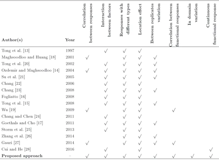
cross-validation method [30]. In this method, data is partitioned into k sets of equal size. Then, in each iteration, k 1 data sets are used to estimate the polynomial regression and one set is used as test set to nd the SSE. This process is repeated k times with dierent test sets and the average of all SSEs is used to evaluate the accuracy and precision of the estimation. It should be noted that the number of data should be large enough to use this method. Step 2: Calculating a new index for functional responses. Consider the example in Figure 1 is comprised of an NTB functional response, f, and its target function. If the researcher only considers the four discrete levels of the signal factor, t, shown in the gure, there is a negligible dierence between es-timated and target functions. However, it is obvious that the estimated function deviates from its target. As a proposed solution, the area enclosed between the two functions is considered as a deviation measure. Therefore, for the NTB type functional responses, cross points of tted and target functions should be found. To do this, MATLAB software can be used to nd roots of the obtained equation by subtracting the tted function from the target one. The next step is aggregating the absolute values of integrals between roots as deviation measure. If we are only interested in the location eect and there are not any additional response variables, the treatment with the minimum Aggregated Absolute Integral Value (AAIV) can be selected as the best. By considering one functional re-sponse in the problem, the AAIV for the lth replicate of the kth treatment may be calculated as follows:
AAIVhkl=
X
i;j
j
Z
i
(Th(t) f^hkl(t))dt
; (3)
where i; j are two consecutive cross points of the tar-get and estimated functions, Th(t) is target function
of the hth functional response, and ^fhkl(t) is
esti-mated function of the hth response for the lth repli-cate in the kth treatment. Note that in the problems
Figure 1. A sample of estimated functional response with target function.
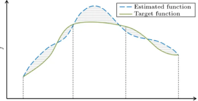
Figure 2. Two dierent functions with equal AAIVs but dierent shapes.
with more than one functional response, AAIV is cal-culated for each response separately and, then, overall index is calculated as expressed in the next step.
There are two dierent dispersion eects in the considered problem. The rst one is IDV, which is related to the dierence in deviation of estimated function from target in the signals domain. To consider it, the maximum dierence between target and estimated functions obtained by considering all replicates may be added in the new index. This can help to distinguish sudden changes of deviation between estimated and target functions. For better il-lustration, two estimated functions with equal AAIV values have been depicted in Figure 2. The estimated function for treatment 1 is very close to the target function in most of its signal levels, but there is a large deviation for some levels, so it is clear that the proposed index should consider such deviations. In addition, the deviation between the target and esti-mated functions for treatment 2 is almost constant throughout the dierent signal levels, which may be preferable since both treatments have equal AAIV values. Furthermore, in some cases, positive or nega-tive deviations may have various importance and we modify the proposed index to a Weighted Aggregated Absolute Integral Value (WAAIV) as follows:
WAAIVhkl=w1
X
i;j j
Z
i
Th(t) f^hkl(t)
dM
!
+ w2
X
p;q q
Z
p
^
fhkl(t) Th(t)
dM
!
+ w3maxtTh(t) f^hkl(t);
(4) where i and j are two consecutive cross points where target function of the hth functional response Th(t)
is above the estimated function of the hth functional response for the lth replicate in kth treatment ^fhkl(t)
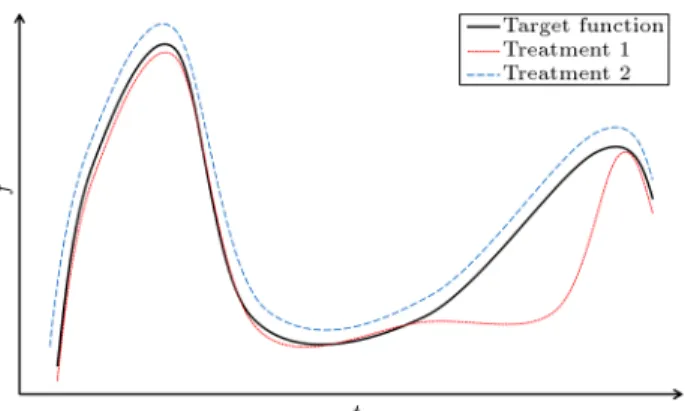
Figure 3. Three estimated functions for dierent replicates of a treatment.
and p; q, are two consecutive cross points where the mentioned target function is below the mentioned estimated function; and w1, w2, and w3 are weight
coecients for the negative, positive, and in domain variations, respectively.
The second type of dispersion eect is BRV and may be considered when there are dierent estimated functions for each treatment because of replicates. For better comprehension, consider Figure 3. This type of dispersion eect is incorporated in the next step of the proposed method.
Some of the problems may have STB or LTB-type functional responses. For example, consider the air pollution rate through the time. It is desired that this value should be near zero throughout the whole signal domain. Thus, it may be considered as an STB functional response. In such cases, the AAIV index may be simply obtained by calculating the area under the tted curve in each treatment. Note that we aim to minimize the AAIV for STB or NTB-type functional responses while it is desired to maximize it for LTB-type functional responses. Step 3: Constructing the overall index for multiple responses. In this step, all calculated indices for dierent responses should be summarized in a total index. However, there are two possible situations here. In the rst case, responses are uncorrelated and in the second one, they have a signicant correlation structure. In the rst case, the desirability measure is employed. To calculate the desirability of STB, LTB, and NTB-type classic responses, the proposed indices by Derringer and Suich [2] are used. In addition, the desirability for an NTB or STB functional response may be calculated based on Derringer and Suich [2] as follows:
dmh;k=
8 < :
UMh Mh;k
UMh
0 < Mh;k< UMh
0 Mh;k> UMh
; (5) where Mh;k is the average of AAIV (or WAAIV)
values of the hth functional response in the kth treatment, UMh is the upper specication limit for
Mh;k, and is the shape constant of the desirability
function.
In the case of problems with two or more replicates in each treatment, we also have variance for AAIV (or WAAIV) values in each treatment. Hence, to incorporate the BRV as the second type of dispersion eect in the problems with uncorrelated responses, we consider the variance of the AAIV (or WAAIV) for each functional response as an STB-type response, and then calculate its desirability as follows.
dh;k=
8 < :
UVh Vh;k
UVh
0 < Vh;k< UVh
0 Vh;k> UVh
; (6)
where Vh;k is the variance of AAIV (or WAAIV)
values of the hth functional response in the kth treatment, UVh is the upper specication limit for
Vh;k, and is the shape constant of the desirability
function.
To calculate the overall desirability, D, at each treatment, Derringer [31] proposed a modied geometric average with weighting terms, which is employed in this paper as well.
In the second case, there are correlated re-sponses and thus, the previous approach is not recom-mended because it ignores the correlation structure of responses. To consider multiple correlated responses, Chiao and Hamada [32] proposed a method in which the treatment with maximum probability of being all responses in the corresponding specication limits is selected as the best solution. The probability is calcu-lated by considering multivariate normal distribution, which considers the covariance matrix of responses. Hence, the correlation structure is considered as well as the BRV in the calculations. The Proportion Of Conformance (POC) for correlated responses in the kth treatment can be calculated as follows:
POCk = P (y 2 E j xk); (7)
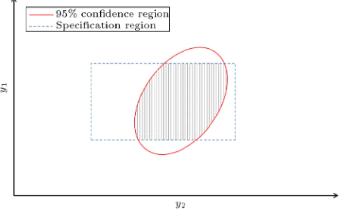
where y is the vector of classic responses and E is the corresponding specication region. For better comprehension, consider two correlated y1,
y2 responses with specication region and 95%
condence interval as shown in Figure 4. The shared area, which is illustrated with dashes, shows the proportion of conformance.
On the other hand, when the functional responses correlate, we should compute the covariance matrix of AAIVs (or WAAIVs) through the replicated data. It should be noted that before calculating the POC index for AAIVs (or WAAIVs), we should check the normality assumption for them. If the AAIVs (or WAAIVs) do not follow a normal
Figure 4. Proportions of conformance for two supposed responses.
distribution, we should use a transformation method. Then, the Proportion Of Conformance (POC) for each treatment can be calculated by replacing y with AAIV (or WAAIV) in Eq. (7). Note that the specication region for AAIV (or WAAIV) is in the form of [0 bh]m, where bhis the desired upper bound
for AAIVhkl (or WAAIVhkl) dened by the analyst.
Step 4: Optimizing the overall index to nd the best setting. By doing the previous steps, the analyzer can select the best treatment based on the overall index. However, if the analyzer wants to search for a better setting in the whole solution space, they may run this step. Before running the optimization algorithm, a relation function between controllable factors and calculated indices (POC or total desirability) should be estimated. The nal step is employing an algorithm to nd the best settings for the controllable factors. Genetic Algorithm (GA) is one of the popular methods to search for near-optimal solution in the problems with discrete or continuous solution spaces. In each iteration, it makes better solutions using crossover and mutation operators. There are several examples of using GA in multi-response optimization problems. For example, refer to [6,33-36]. However, it should be noted that GA is not the only alternative and the optimization algorithm may be selected by the analyst based on their preferences and the problem conditions. Thus, we recommend it to search for the optimum total index. It should be noted that tuning of GA parameters is performed using the Taguchi method. In this method, through a factorial design, the mean of calculated responses in each try for dierent parameter levels is computed and the best level for each parameter is selected. 4. Numerical examples
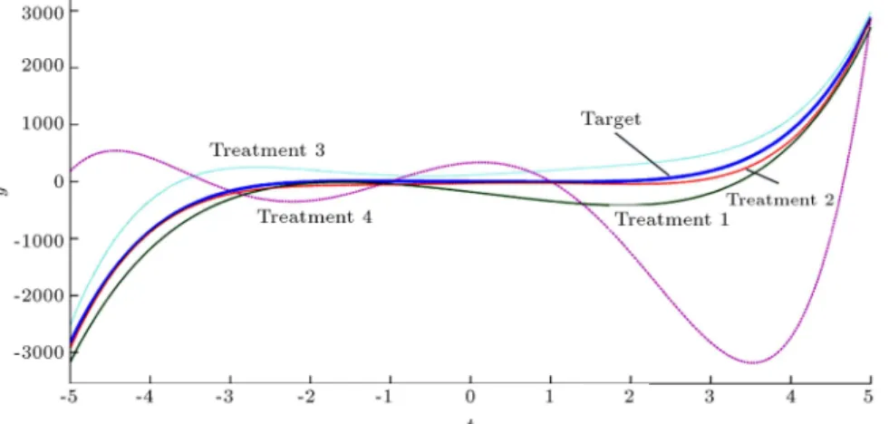
4.1. Example 1: Performance evaluation As the rst example, suppose a 22factorial design with
Figure 5. Target function versus tted functions for dierent treatments in Example 1.
Table 2. Experimental design of Example 1
Treatment x1 x2 t = 5 t = 3 t = 1 t = 1 t = 3 t = 5 SSE
1 1 1 {3168.01 {305.97 {42.02 {342.23 {202.08 2711.04 4:56 10 25
2 1 {1 {2927.91 {216.87 {52.45 {22.69 57.38 2871.99 4:31 10 25
3 {1 1 {2527.56 234.19 109.01 197.67 488.40 2982.20 7:51 10 25
4 {1 {1 186.15 {162.13 4.32 2.83 {2826.86 2876.91 7:76 10 23
response y. It is supposed that the target function for y is t5 2t3+t2 4t+1:5. To evaluate the performance of
the proposed method, suppose that we know the exact functional response corresponding to each treatment as shown in Eqs. (8)-(11), respectively:
0:6149 t5+ 0:3904 t4+ 14:7584 t3
11:6588 t2 165:2982t 181:4266; (8)
1:2314 t5+ 0:3522 t4 8:4762 t3
8:7811 t2 22:2397 t 29:3061; (9)
1:3374 t5 1:4330 t4+ 13:6787 t3
+ 40:3379 t2 57:1314 t 113:9450; (10)
4:1653 t5+ 15:6840 t4 97:0485 t3
344:1352 t2 91:9832 t 331:6912: (11)
Figure 5 shows the target and treatment functions. For the rst evaluation, we consider ( 5, 3, 1, 1, 3, 5) as initial signal levels to generate response values and add a standard normal residual to them. The resulting response values under dierent signal levels are reported in Table 2.
To evaluate the eciency of the proposed mea-sure, we compare it with HD proposed by Fogliatto [16].
The HD between two vectors y1 and y2 is calculated
as follows:
h(y1; y2) = max
max
y12y1
min
y22y2
q
(y1 y2)2
; max
y22y2
min
y12y1
q
(y1 y2)2
; (12)
As can be seen in Eq. (12), HD uses two points, which have minimum deviation from each other, to calculate the distance between the two vectors and ignores the order of points. For example, by considering y1 = (2; 10; 5) and y2 = (10; 5; 2), the result is
h(y1; y2) = 0; however, it is obvious that they are
dierent. To calculate the AAIV for each treatment, we estimate a function for it based on the results reported in Table 2. The goodness of tness is evaluated through the sum of squared dierences between each observation and its estimated value (SSE), which is reported in Table 2 as well. Table 3 shows the AAIV and HD for each treatment. It can be seen that using the HD (based on [16]) as comparing measure leads to selecting treatment 4 as the best one. However, it is obvious from Figure 5 that it is not the best choice. This shows that the HD is not an ecient measure in such problems. Another conict of results can be seen between treatments 1 and 3. Based on the AAIV measure, treatment 1 dominates 3, but based on the HD measure, the result is the opposite. This is another problem with employing HD and occurs due
Table 3. AAIV and HD results for each treatment in Example 1 by considering [ 5, 5] as signal domain.
Treatment x1 x2 AAIV HD
1 1 1 2389.98 339.51
2 1 {1 681.02 130.11
3 {1 1 2615.77 300.93
4 {1 {1 12180.79 5.32
Figure 6. AAIV changes due to change in signal levels.
Figure 7. HD changes due to change in signal levels.
to its discrete nature. To compare the variations of AAIV and HD results, we change each signal level in a specied interval [ 0:5, 0:5]. Hence, the signal levels is changed from ( 5:5, 3:5, 1:5, 0.5, 2.5, 4.5) to ( 4:5, 2:5, 0:5, 1.5, 3.5, 5.5) in 10 iterations. As shown in Figure 6, by changing the signal levels, AAIVs are approximately robust against the added values to the initial signal levels; however, the changes in HD according to the signal level shifts are considerable as shown in Figure 7. This shows that HD is related to signal levels and the best treatment may be changed by selecting dierent signal levels, but AAIV is more robust. Nonetheless, HD may be a good choice in the cases that we deal with monotonic functions for the treatments. In such problems, response values in dierent signal levels may be far from each other and, hence, ignoring the order due to the use of HD cannot aect the selected solution. For better illustration, consider [4, 5] as limit of signal domain. As can be seen in Figure 5, all of the functions are monotonic in this range. To compute the HD and AAIV in this
Table 4. AAIV and HD results for each treatment in Example 1 by considering [4, 5] as signal domain.
Treatment x1 x2 AAIV HD
1 1 1 195.55 251.74
2 1 {1 115.76 169.40
3 {1 1 156.65 218.50
4 {1 {1 2350.59 3633.97 Table 5. Supposed experimental results for each signal level in Example 2.
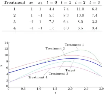
Treatment x1 x2 t = 0 t = 1 t = 2 t = 3
1 1 1 4.4 7.4 11.0 6.3
2 1 {1 5.5 8.3 10.0 7.4
3 {1 1 7.3 6.4 8.0 3.3
4 {1 {1 1.5 5.0 6.5 3.4
Figure 8. Fitted functional responses in Example 2.
range, we consider (4, 4.2, 4.4, 4.6, 4.8, 5) as signal levels and generate response values based on Eqs. (9)-(12) by adding standard normal residuals to them. It can be seen in Table 4 that HD results conrm the AAIV results. It should be noted that although the proposed method considers the continuous nature of the responses, it may incorporate an estimation error in the calculations. Therefore, it is very important to nd an estimated function with acceptably small error. 4.2. Example 2: In-domain dispersion eect Suppose that there is a problem with one functional response and two controllable factors. The functional response is aected by a signal factor (t) with four levels (0, 1, 2, 3). The target values are supposed to be (4.5 , 7.3, 9, 6.4) and the experimental results are supposed as reported in Table 5. Suppose that the analyst is interested in ranking treatments by considering deviation from target as well as IDV. By considering polynomial order equal to 6, the SSE values are approximately zero and each function has only one maximum point. Hence, we are not worried about overtting. Figure 8 illustrates the tted functions for target and treatments. As can be seen, the tted responses corresponding to treatments 1 and 2 have
small deviations from the target in comparison with treatments 3 and 4.
To better illustrate the eciency of the proposed measure, consider another approach from the literature with discrete viewpoint to the signal levels. Wu [19] proposed an approach for optimizing multiple func-tional responses using double-exponential desirability function. Based on his proposition, the desirability for the kth treatment by considering NTB type uncorre-lated responses is calcuuncorre-lated as follows:
W Dk=
" m h=1
u=1exp ( chjyhku ghuj h) 1 # 1 m ; (13) where yhkuis the value of the hth response for the uth
signal level in treatment k, ghu is target value of the
hth response for the uth signal level, is number of signal levels, m is number of functional responses, h
is shape constant of the hth response, and ch is scale
constant of the hth response.
Using the predened equations, WD (by consider-ing h= ch= 1), AAIV, and WAAIV (by considering
[0.2 0.2 0.6] as weight vector) are calculated and the results are summarized in Table 6. Based on the WD results, treatment 1 is selected as the best by a wide dierence from the second treatment. This is
Table 6. The results of dierent measures in Example 2.
Treatment WD AAIV WAAIV
1 0.56 3.25 2.39
2 0.37 3.00 1.20
3 0.12 5.20 3.96
4 0.07 7.89 3.67
because of ignoring the IDV. By employing the AAIV, treatment 2 may be selected as the best while it has a negligible dierence from treatment 1. However, by employing the WAAIV, which can consider the comments of the analyst as weights, it can be seen that treatment 2 is very better than treatment 1.
4.3. Example 3: Correlated functional responses
Expand Example 1 to include two controllable factors, x1 and x2, a signal factor, t, and two correlated
functional responses, y1 and y2. Target proles for
functional responses are T1= t5+2t4+3t3 2t2+t+2:5
and T2 = t5 2t3+ t2 4t + 1:5, respectively, which
are depicted in Figure 9. The covariance matrix of the response functions is
10 11:4 11:4 18
. By replicating the experiment in each signal level of each treatment for 10 times, mean m and covariance matrix s of the functional responses may be estimated based on the observed values of the responses. Table 7 shows the experimental design, including mean and covariance
Figure 9. Target proles for functional responses in Example 3.
Table 7. Experimental design of Example 3.
Treatment t = 5 t = 3 t = 1 t = 1 t = 3 t = 5
1 M 0= " 2301:18 2826:89 #
M0= "
180:81 166:27 #
M0= "
3:49 650 #
M0= "
7:22 2:64
#
M0= "
475:95 191:01 #
M0= " 4707:80 2881:95 # S = " 3:57 5:81 5:81 9:85 # S = " 7:90 8:38 8:38 11:47 # S = " 7:17 9:44 9:44 13:30 # S = " 9:85 14:92 14:92 24:29 # S = " 6:03 7:40 7:40 9:28 # S = " 8:18 10:27 10:27 14:02 # 2 M 0= " 2304:83 2832:15 #
M0= "
180:97 167:51 #
M0= "
2:31 7:71
#
M0= "
8:84 1:23
#
M0= "
471:24 184:15 #
M0= " 4710:44 2885:08 # S = " 1:83 2:64 2:64 4:64 # S = " 5:49 6:98 6:98 9:88 # S = " 15:68 19:25 19:25 24:77 # S = " 6:81 7:81 7:81 10:12 # S = " 17:07 21:63 21:63 28:13 # S = " 13:23 16:41 16:41 21:56 # 3
M0= "
2302:74 2829:05 #
M0= "
180:66 166:38 #
M0= "
2:24 8:71
#
M0= "
7:78 1:73
#
M0= "
474:01 188:15 #
M0= " 4705:18 2878:56 # S = " 18:01 24:57 24:57 35:46 # S = " 12:97 17:42 17:42 24:00 # S = " 8:95 12:69 12:69 19:47 # S = " 6:05 7:86 7:86 11:60 # S = " 6:72 8:83 8:83 12:20 # S = " 4:61 6:85 6:85 10:64 # 4
M0= "
2302:89 2828:66 #
M0= "
181:45 168:18 #
M0= "
2:00 7:66
#
M0= "
6:69 4:18
#
M0= "
471:89 185:19 #
M0= " 4708:43 2883:12 # S = " 6:47 7:32 7:32 8:73 # S = " 13:21 16:81 16:81 21:84 # S = " 6:29 8:84 8:84 13:28 # S = " 4:92 5:66 5:66 7:45 # S = " 14:01 19:17 19:17 27:00 # S = " 6:24 8:38 8:38 11:93 #
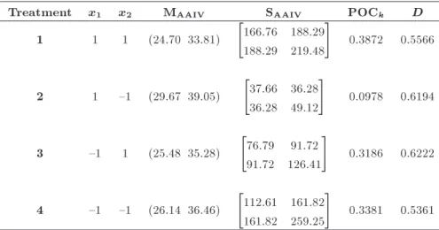
Table 8. AAIVs and POC results in Example 3.
Treatment x1 x2 MAAIV SAAIV POCk D
1 1 1 (24.70 33.81)
"
166:76 188:29 188:29 219:48 #
0.3872 0.5566
2 1 {1 (29.67 39.05) "
37:66 36:28 36:28 49:12 #
0.0978 0.6194
3 {1 1 (25.48 35.28) "
76:79 91:72 91:72 126:41
#
0.3186 0.6222
4 {1 {1 (26.14 36.46) "
112:61 161:82 161:82 259:25 #
0.3381 0.5361
Table 9. Polynomial regression parameters corresponding to each treatment in Example 4.
Treatment x1 x2 x3 B
1 {1 {1 {1 [{5.74, {50.91, 784.57, 1201, 10724.97, {51981.87, {22339.75, {128407.13] 2 -1 0 0 [2, {45.91, 300, {3000, 11724.97, {10000, 21000, {120000] 3 -1 1 1 [9.74, {40.91, {184.57, {7201, 12724.97, 31981.87, 64339.75, {111592.87] 4 0 {1 0 [{5, 5, {120, 3501, {2000, 1000, {48339.75, 110000]
5 0 0 1 [2.74, 10, {604.57, {700, {1000, 42981.87,{5000, 118407.13] 6 0 1 {1 [2.26, {15, 724.57, {2801, 3000, {43981.87, 53339.75, {228407.13] 7 1 {1 1 [{4.26, 60.91, {1024.57, 5801, {14724.97, 53981.87, {74339.75, 348407.13] 8 1 0 {1 [{4.74, 35.91, 304.57, 3700, {10724.97, {32981.87, {16000, 1592.87]
matrices for the functional responses in each signal level.
Now, we estimate the functional responses for each replicate and, then, compute the mean and covariance matrices of the AAIVs for each treatment. To calculate POC, we test the AAIVs for normality and consider [0 30]2 as their desired specication region.
Now, we ignore the covariance structure and calculate the desirabilities to compare the results. To do this for each response, h, a desirability corresponding to mean with UMh = 60 and a desirability corresponding to
variance with UVh = 500 are calculated and the total
desirability is found by considering 0.25 as weight of each desirability. Results are summarized in Table 8; as shown, the rst treatment presents the best POCk
value; however, the third treatment presents the best D value. This shows that ignoring covariance structure in the problems with correlative responses may result in a wrong choice.
4.4. Example 4: Dissolved dose of tablet Suppose the problem of nding the best composition of a tablet comprised of three raw materials x1, x2, and x3, such that the relation between time t and dissolution of tablet y (based on milligrams) follows
a target function, T , given in Eq. (14): T = 1:13 t7+ 29:53 t6 327:45 t5
+ 1999:12 t4 7270:48 t3+ 15805:83 t2
19130:77 t + 110033:64: (14)
We consider an orthogonal array with 8 treatments as experimental design. The polynomial regression parameters, b, for each treatment are given in Table 9. It may be dangerous if the dissolving speed of the tablet is higher than the target or if the dissolution in a time point has a large dierence from its target. Hence, we should assign a larger weight to integral values when the target function is below the treatment function. Also, the maximum dierence should be considered as well, because increasing the speed of dissolution may be dangerous. Since there is only one functional response in this problem, we do not need to construct the overall index and optimization may be done on the WAAIV. By considering [0.1, 18, 3] as the weight vector and [0, 10] as range, WAAIVs are calculated with the results given in Table 10. The estimate of WAAIV is obtained using ordinary least squares method after removing the terms with large p-values (p-values are provided
Table 10. WAAIV for each treatment in Example 4. Treatment x1 x2 x3 WAAIV
1 1 1 1 797098.7
2 1 0 0 443368.4
3 1 1 1 700695.5
4 0 1 0 427297.3
5 0 0 1 5783643.0
6 0 1 1 1733688.0
7 1 1 1 14908102.0
8 1 0 1 1096071.0
Table 11. Experimental design of the problem. Treatment x1 x2 x3 y1 y2 y3
1 {1 {1 {1 5.1 8.3 0.78
2 {1 1 {1 5.4 8.24 0.72
3 1 {1 {1 6.1 8.49 0.7
4 1 1 {1 6.2 8.48 0.77
5 0 0 {1 5.6 8.17 0.78
6 {1.41 0 1 5.8 9 0.65
7 1.41 0 1 7.3 9.56 0.67
8 0 {1.41 1 7.6 9.28 0.69
9 0 1.41 1 7.9 9.62 0.65
10 0 0 1 5.1 8.95 0.62
in parentheses), as follows:
WdAAIV = 3679816(0:006) + 3548565x1(0:016)
+ 2960930x3(0:021)
+3477109x1x3(0:024); R2=91:40%: (15)
Finally, by employing GA with population size of 1000, and crossover and mutation rates of 0.7 and 0.4, after 60 iterations, we achieve [{0.9605, 0.2288, 0.7172] as the best factors levels array with WAAIV equal to 45.7711. A conrmation experiment may be performed to check the validity of the GA result.
5. A real case
Consider the real case given by Fogliatto [16] from the pet food production industry about the development of an alternative formula for a well-known brand of dog biscuits. The percentages of three ingredients are rewritten as two mixture variables and, thus, by considering the biscuit thickness, there are three con-trollable factors. Levels are dened based on a Central Composite Design (CCD) including ten treatments illustrated in Table 11.
There are three real responses and a simulated functional response in this problem. Response types
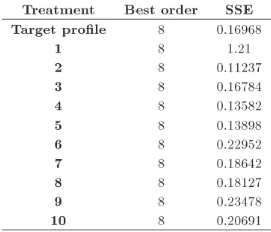
Table 12. Best tting order for each target and treatment.
Treatment Best order SSE
Target prole 8 0.16968
1 8 1.21
2 8 0.11237
3 8 0.16784
4 8 0.13582
5 8 0.13898
6 8 0.22952
7 8 0.18642
8 8 0.18127
9 8 0.23478
10 8 0.20691
and specications are as follows: y1 is
nominal-the-best (U1 = 8; m1 = 7:5; L1 = 5), y2 is
nominal-the-best (U2 = 10; m2 = 9:5; L2 = 8), and y3 is
larger-the-better (U3= 0:8; L3= 0:6), where miis the
target value and Ui and Li are the upper and lower
specication limits of the ith response, respectively. Note that the values of functional response in signal levels are driven from Table AI of Fogliatto [16].
As expressed in the previous section, the next step is nding the best t with the best order for each treatment. To avoid overtting, we limit the maximum order of functions between 5 and 9. Table 12 shows the best order with corresponding SSE for each treatment. Figure 10 shows the tted functions for target and the other treatments. The shapes of tted functions are smooth enough and there are not several maximum or minimum points for each function. Hence, overtting is unlikely. It can be seen that tted prole of the treatment 3 can visually be selected as the nearest prole to the target.
The next step is calculating the absolute integral value between target prole and each of the treatments from one cross point to the next one. To do this, cross points between target and each of proles should be found. After that, aggregating absolute integral values and selecting the treatment with minimum AAIV are desirable. Table 13 shows the cross points and AAIV for each of the treatments. It should be mentioned that lower limit of the integral range is equal to zero and upper limit is assumed to be equal to the number of values in functional response for each treatment.
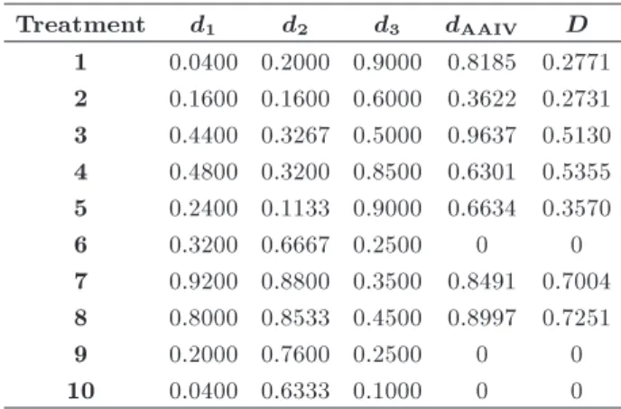
Now, the desirability of each response and AAIV should be calculated for each treatment. Then, we should nd the estimating equation for desirabilities. By considering = 1, and UMh = 25, desirabilities
(di) can be calculated as shown in Table 14. Note
that total desirability (Di) has been calculated by
considering wi = 0:25, which is same as the rst
scenario in Fogliatto [16].
Figure 10. Fitted polynomial proles for target and treatments. Table 13. Cross points and AAIV for each treatment.
Treatment Cross points AAIV
1 1.3011 3.4710 7.7301 20.3327 28.0974 31.5621 3.6308
2 1.2301 38.9803 40.8241 45.0043 12.7561
3 1.3257 34.2576 40.1817 44.7791 0.7264
4 1.2358 37.5111 40.4301 44.8857 7.3987
5 1.2368 37.4034 40.3069 44.8664 6.7312
6 1.2069 40.0524 44.6308 25.8691
7 1.1436 40.1416 44.7220 3.0190
8 1.0653 40.1753 44.7377 2.0058
9 1.2044 40.0414 44.6190 20.0280
10 1.1930 40.0974 44.6747 1080.1195
Table 14. Desirability values for each treatment. Treatment d1 d2 d3 dAAIV D
1 0.0400 0.2000 0.9000 0.8185 0.2771 2 0.1600 0.1600 0.6000 0.3622 0.2731 3 0.4400 0.3267 0.5000 0.9637 0.5130 4 0.4800 0.3200 0.8500 0.6301 0.5355 5 0.2400 0.1133 0.9000 0.6634 0.3570
6 0.3200 0.6667 0.2500 0 0
7 0.9200 0.8800 0.3500 0.8491 0.7004 8 0.8000 0.8533 0.4500 0.8997 0.7251
9 0.2000 0.7600 0.2500 0 0
10 0.0400 0.6333 0.1000 0 0
as the best one. To search for better treatments, we need to nd tting models for desirabilities. Note that normality assumption cannot be rejected for any of the desirabilities. After tting dierent regression models
and removing terms with large p-values (p-values are provided in parentheses), we nd the following equa-tions with acceptable coecients of determination, R2:
^
d1= 0:26556 (0:042) + 0:19633x1(0:046);
R2= 81:42%; (16)
^
d2=0:373323 (0:015) + 0:073657x1(0:037)
+ 0:267682x3(0:009) + 0:0656x21(0:055)
+ 0:082349x2
2(0:044); R
2= 99:98%; (17)
^
d3=0:515 (0:000) 0:235x3 (0:003)
Figure 11. Changes in total desirability and controllable factors versus iteration numbers.
^
dAAIV=0:51867 (0:000) + 0:20219x1(0:035)
0:25808x2(0:013) 0:16891x3(0:044);
R2= 86:67%: (19)
To prevent unreal results, we set 1 for di> 1 and
0 for di< 0. Now, we can search for better treatments.
To do this, we employ GA with population size of 1000, and crossover and mutation rates of 0.7 and 0.4, respectively. After 60 iterations, we nd a treatment with x1= 1:41, x2= 1:41, x3 = 0:69, and ^D=0.6487
as the best result. Note that although based on Table 14, the total desirability of treatment 8 is 0.7251, we nd ^D=0.6487 for it. Hence, it is necessary to do a real experiment with the setting of x1 = 1:41, x2 = 1:41,
and x3 = 0:69 to nd the exact total desirability
value and compare it with treatment 8. Figure 11 shows the changes in total desirability and controllable factors in each treatment versus iteration numbers. As can be seen, increasing x1 and x2 will increase total
desirability.
It should be noted that in [16], treatment 8 is selected as the best by considering equal weights for calculating total desirability. By solely considering functional response, Fogiatto [16] found treatment 4 using maximum and summation operators and treat-ment 5 using average operator as the best. However, as can be seen in Table 13, we nd treatment 3 as the best by solely considering functional response. Hence, it can be concluded that nding treatment 8 as best by both methods is because of other responses (i.e. y1, y2,
and y3).
6. Conclusion and future researches
We proposed a novel method for optimizing multi-response problems with continuous functional
re-sponse(s) and considered two dierent dispersion ef-fects. The rst dispersion eect was \In Domain Variation (IDV)," which was related to the dierence in deviation of estimated function, and the second one was \Between Replicates Variation (BRV)," which might be considered when there were dierent estimated functions for each treatment because of replicates. The rst important step of the proposed method was nding an acceptable polynomial tting model for functional response in each treatment from the observed values. Thus, if we could not nd tted functions with acceptable estimating errors, the pro-posed method might not be applicable. We found the cross points between target function(s) and estimated function(s) in each treatment. Thereafter, we proposed the absolute integral value as the measure. In some special problems, it was important to distinguish be-tween positive and negative deviations from the target function. Moreover, IDV might be considered in this step. For analyzing such cases, WAAIV was proposed. To aggregate uncorrelated AAIVs (or WAAIVs) in one measure, we used desirability function. In the problems with correlated functional responses, we em-ployed Proportion Of Conformance (POC) proposed by Chiao and Hamada [32] to transform correlated AAIVs (or WAAIVs) into one measure. The BRV might be considered in this step. Finally, we applied GA to nd the best levels for factors. Some illustrative examples showed that our proposed continuous method was ecient in the problems with functional responses. The application of the proposed method was illustrated through a real case in pet food production extracted from [16]. In this paper, we supposed that the eect of nuisance factor was randomly distributed through the randomization. Considering these factors in the proposed method can be a direction for future research. Moreover, we supposed that there was a polynomial
relation between functional response and the signal factor. A future study may be done to focus on other types of estimated functions and use spline regression to model the functional responses. In addition, investi-gating the multi-response problems with correlational structure between classic and functional responses can be a fruitful area of research.
References
1. Harrington, E. \The desirability function", Industrial Quality Control, 21(10), pp. 494-498 (1965).
2. Derringer, G. and Suich, R. \Simultaneous optimiza-tion of several response variables", Journal of Quality Technology, 12(4), pp. 214-219 (1980).
3. Del Castillo, E., Montgomery, D.C., and McCarville, D.R. \Modied desirability functions for multiple re-sponse optimization", Journal of Quality Technology, 28(3), pp. 337-345 (1996).
4. Jeong, I.J. and Kim, K.J. \Interactive desirability function approach to multi-response surface optimiza-tion", International Journal of Reliability, Quality and Safety Engineering, 10(02), pp. 205-217 (2003). 5. Ribardo, C. and Allen, T.T. \An alternative
desirabil-ity function for achieving `six sigma' qualdesirabil-ity", Qualdesirabil-ity and Reliability Engineering International, 19(3), pp. 227-240 (2003).
6. Noorossana, R., Tajbakhsh, S.D., and Saghaei, A. \An articial neural network approach to multiple-response optimization", The International Journal of Advanced Manufacturing Technology, 40(11-12), pp. 1227-1238 (2009).
7. Mostafa, J.J., Mohammad, M.A., and Ehsan, M. \A hybrid response surface methodology and simulated annealing algorithm: A case study on the optimization of shrinkage and warpage of a fuel lter", World Ap-plied Sciences Journal, 13(10), pp. 2156-2163 (2011). 8. He, Z., Zhu, P.F., and Park, S.H. \A robust desirability
function method for multi-response surface optimiza-tion considering model uncertainty", European Journal of Operational Research, 221(1), pp. 241-247 (2012). 9. Chen, H.W., Xu, H., and Wong, W.K.
\Balanc-ing location and dispersion eects for multiple re-sponses", Quality and Reliability Engineering Interna-tional, 29(4), pp. 607-615 (2013).
10. Costa, N.R., Lourenco, J., and Pereira, Z.L. \Desir-ability function approach: A review and performance evaluation in adverse conditions", Chemometrics and Intelligent Laboratory Systems, 107(2), pp. 234-244 (2011).
11. Taguchi, G., Taguchi Methods: Signal-to-Noise Ratio for Quality Evaluation, 1st Ed. 3, Dearborn: American Supplier Inst. (1991).
12. Miller, A. and Wu, C. J. \Parameter design for signal-response systems: a dierent look at Taguchi's dynamic parameter design", Statistical Science, 11(2), pp. 122-136 (1996).
13. Tong, L.I., Su, C.T., and Wang, C.-H. \The opti-mization of multi-response problems in the Taguchi method", International Journal of Quality & Reliabil-ity Management, 14(4), pp. 367-380 (1997).
14. Ozdemir, G. and Maghsoodloo, S. \Quadratic quality loss functions and signal-to-noise ratios for a trivariate response", Journal of Manufacturing Systems, 23(2), pp. 144-171 (2004).
15. Tong, L.I., Wang, C.H., and Tsai, C.W. \Robust de-sign for multiple dynamic quality characteristics using data envelopment analysis", Quality and Reliability Engineering International, 24(5), pp. 557-571 (2008). 16. Fogliatto, F.S. \Multiresponse optimization of
prod-ucts with functional quality characteristics", Quality and Reliability Engineering International, 24(8), pp. 927-939 (2008).
17. Goethals, P.L. and Cho, B.R. \The development of a robust design methodology for time-oriented dynamic quality characteristics with a target prole", Quality and Reliability Engineering International, 27(4), pp. 403-414 (2011).
18. Maghsoodloo, S. and Huang, L.-H. \Quality loss func-tions and performance measures for a mixed bivariate response", Journal of Manufacturing Systems, 20(2), pp. 73-88 (2001).
19. Wu, F.C. \Robust design of nonlinear multiple dy-namic quality characteristics", Computers & Industrial Engineering, 56(4), pp. 1328-1332 (2009).
20. Tong, L.I., Wang, C.H., Houng, J.Y., and Chen, J.Y. \Optimizing dynamic multiresponse problems using the dual-response-surface method", Quality Engineer-ing, 14(1), pp. 115-125 (2002).
21. Su, C.-T., Chen, M.C., and Chan, H.-L. \Applying neural network and scatter search to optimize parame-ter design with dynamic characparame-teristics", Journal of the Operational Research Society, 56(10), pp. 1132-1140 (2005).
22. Chang, H.-H. \Dynamic multi-response experiments by backpropagation networks and desirability func-tions", Journal of the Chinese Institute of Industrial Engineers, 23(4), pp. 280-288 (2006).
23. Chang, H.H. \A data mining approach to dynamic multiple responses in Taguchi experimental design", Expert Systems with Applications, 35(3), pp. 1095-1103 (2008).
24. Chang, H.H. and Chen, Y.K. \Neuro-genetic approach to optimize parameter design of dynamic multire-sponse experiments", Applied Soft Computing, 11(1), pp. 436-442 (2011).
25. Storm, S.M., Hill, R.R., and Pignatiello, J.J. \A response surface methodology for modeling time series response data", Quality and Reliability Engineering International, 29(5), pp. 771-778 (2013).
26. Zhang, L.Y., Ma, Y.-Z., Zhu, L.-Y., and Wang, J.J., \A modied particle swarm optimization algorithm for dynamic multiresponse optimization based on goal
programming approach", Proceedings of 2014 IEEE International Conference on Management Science & Engineering (ICMSE), Singapore, pp. 160-166 (2014). 27. Gauri, S. \Optimization of multi-response dynamic systems using principal component analysis (PCA)-based utility theory approach", International Journal of Industrial Engineering Computations, 5(1), pp. 101-114 (2014).
28. Cui, Q.A. and He, B. \Modeling and optimization of functional response based on kriging model", In Proceedings of the 22nd International Conference on Industrial Engineering and Engineering Management 2015: Core Theory and Applications of Industrial Engineering 1, E. Qi, J. Shen, and R. Dou, Eds., Ed. Paris: Atlantis Press, pp. 3-14 (2016).
29. Kang, L. and Albin, S. \On-line monitoring when the process yields a linear", Journal of Quality Technology, 32(4), pp. 418-426 (2000).
30. Stone, M. \Cross-validatory choice and assessment of statistical predictions", Journal of the Royal Statistical Society; Series B (Methodological), 36(2), pp. 111-147 (1974).
31. Derringer, G.C. \A balancing act-optimizing a prod-ucts properties", Quality Progress, 27(6), pp. 51-58 (1994).
32. Chiao, C.H. and Hamada, M. \Analyzing experiments with correlated multiple responses", Journal of Quality Technology, 33(4), pp. 451-465 (2001).
33. Cheng, C.-B., Cheng, C.-J., and Lee, E. \Neuro-fuzzy and genetic algorithm in multiple response optimiza-tion", Computers & Mathematics with Applications, 44(12), pp. 1503-1514 (2002).
34. Pasandideh, S.H.R. and Niaki, S.T.A. \Multi-response simulation optimization using genetic algorithm within desirability function framework", Applied Mathematics and Computation, 175(1), pp. 366-382 (2006). 35. Salmasnia, A., Baradaran Kazemzadeh, R., and
Mo-hajer Tabrizi, M. \A novel approach for optimization of correlated multiple responses based on desirability function and fuzzy logics", Neurocomputing, 91(0), pp. 56-66 (2012).
36. Ouyang, L., Ma, Y., and Byun, J.H. \An integrative loss function approach to multi-response optimiza-tion", Quality and Reliability Engineering Interna-tional, 31(2), pp. 193-204 (2015).
Biographies
Mohammad Hasan Bakhtiarifar received his BS degree from Imam Hussein University, Tehran, Iran, and his MS degree in Industrial Engineering from Shahed University in Tehran, Iran, where he is cur-rently a PhD degree student in the same subject. His research interests include design of experiments, multiple-response optimization, multivariate probabil-ities, and metaheuristic algorithms.
Mahdi Bashiri is a Professor of Industrial Engi-neering at Shahed University. He holds a BSc in Industrial Engineering from Iran University of Science and Technology, MSc and PhD from Tarbiat Modarres University. He is a recipient of the 2013 Young National Top Scientist Award from the Academy of Sciences of the Islamic Republic of Iran. He serves as the Editor-in-Chief of Journal of Quality Engineering and Production Optimization published in Iran, and the Editorial Board member of some reputable academic journals. His research interests are facilities planning, stochastic optimization, meta-heuristics, and multi-response optimization. He published about 10 books and more than 190 papers in reputable academic journals and conferences.
Amirhossein Amiri is an Associated Professor at Shahed University in Iran. He received the BS degree from Khajeh Nasir University of Technology; MS degree from Iran University of Science and Technology; and PhD degree from Tarbiat Modares University, all in Industrial Engineering. He is a member of the Iranian Statistical Association. His research interests are statistical quality control, prole monitoring, and Six Sigma.