Vol. 7, No. 1, pp 1- 20 Autumn 2014
A hybrid ant colony optimization algorithm to optimize capacitated
lot-sizing problem
Vahid Hajipour, Parviz Fattahi*, Arash Nobari
Industrial Engineering Department, Faculty of Engineering, Bu-Ali Sina University, Hamedan, Iran
[email protected], [email protected], [email protected]
Abstract
The economical determination of lot size with capacity constraints is a frequently complex, problem in the real world. In this paper, a multi-level problem of lot-sizing with capacity constraints in a finite planning horizon is investigated. A combination of ant colony algorithm and a heuristic method called shifting technique is proposed for solving the problem. The parameters, including the costs, demands and capacity of resources vary during the time. The goal is to determine the economical lot size value of each product in each period, so that besides fulfilling all the needs of customers, the total cost of the system is minimized. To evaluate the performance of the proposed algorithm, an example is used and the results are compared other algorithms such as: Tabu search (TS), simulated annealing (SA), and genetic algorithm (GA). The results are also compared with the exact solution obtained from the Lagrangian relaxation method. The computational results indicate that the efficiency of the proposed method in comparison to other meta-heuristics.
Keywords: Production planning, Capacitated lot-sizing, Ant colony algorithm,
Shifting technique
1. Introduction
The production planning is the process of determining the right amount of the production resources in order to achieve the main objectives of production, i.e. time and quantity of production, the production requirements and the anticipated amount of sales, in a time period called the planning horizon. These problems are generally defined in three time intervals such as long-term, medium-term and short-term. The long-term problem includes the decisions of fulfilling the requirements and effective factors in the long term, such as the site selection for the factory, procurement of equipment, selection of the suitable processes, production resources planning, etc. The medium-term problem includes material requirements planning (MRP), determination of the production quantity and the lot
*Corresponding Author
size, optimization of other parameters such as total cost, etc. Finally, the last type which is the short-term problem consists of day-to-day planning, like the operations sequence planning, etc (Karimi, FatemiGhomi and Wilson, 2003). In this study, we investigate the medium-term production planning problem.
The extent and popularity of material requirements planning in production and industrial systems has led to improving the productivity in production-related activities. The problem of lot size determination, which is used in material requirements planning, specifies how much and when a product should be produced, in order to minimize the costs like the setup cost, production cost, holding cost, etc. Although the lot-sizing procedure is limited by many conditions, including the production conditions or capacity limitations, it was quickly adopted by numerous manufacturing industries and companies for their use in production planning and distribution systems problem (Xie and Dong, 2002).
Determining the correct and appropriate lot size in the production periods is an important factor that affects the performance of the system, its productivity and also the capability and competitiveness of the companies in the market. Therefore, it is essential to develop new methods or improve the existing approaches for the determination of the lot size (Almeder, 2010).
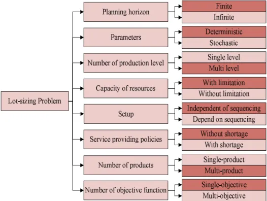
According to the relative researches, lot-sizing problem can be categorized into different cases based on effective factors on the performance and complexity of the problem. Figure 1 indicates various classifications of lot-sizing problem (Karimi, FatemiGhomi and Wilson, 2003).
Figure 1. Classification of lot-sizing problem (Karimi, FatemiGhomi and Wilson, 2003) In a finite horizon lot-sizing problem the demands are usually dynamic and variable with time (Zhou, Lau and Yang, 2004; Wua et al., 2011). Some researchers considered the infinite planning horizon with fixed demands during time (Friedman and Winter, 1978; Gallego and Shaw, 1997). Based on the parameters of the problem, one can take into account deterministic parameters such as demand, cost, capacity, and etc (Teng et al., 1999; Zhou, Lau and Yang, 2004; Robinson, Narayan and Sahin, 2009) and the other one can
consider uncertainty in the parameters (Dellart and Melo 1996; Pai, 2003; Huang and Küçükyavuz, 2008; Senyigit et al., 2013). In the single-level problems, there is no connection between the products in the bill of materials and the final product is often very simple (Billington, McClain andThomas, 1986; Gupta and Keung, 1990; Aggarwal and Park, 1993; Wolsey 1995; Jans and Degraeve, 2004; Brahimi and Dauzere, 2006; Absi and Kedadd-Sidhoum, 2008). With regard to increasing the production levels from the single-level to multi-single-level, the complexity of the problem should be increased, so that problems with multi-level general structures and without capacity constraints can be defined as NP-hard (Dellaert, Jeunet and Jonard, 2000). In the multi-level problems, the production system is made up of components which establish a relationship between the products (Lambrecht, VanderEchen and VanderVeken, 1981; Afentakis, Gavish and Karmarkar, 1984; Rosling, 1986; Dellaert, Jeunet and Jonard, 2000). Some researchers investigated single-product lot-sizing problem (Ganas and Papachristos, 2005; Brahimi and Dauzere, 2006) and the others considered multi-product problems in which manufacturing several products should be planned (Barang, VanRoy and Wolsey, 1984; Jans and Degraeve, 2004; Absi and Kedadd-Sidhoum, 2008; Toledo, Ribeirodo Oliveira and Franca, 2013). Regarding to the capacity of resources, the lot-sizing problems can be categorized into two cases: with capacity constraint (Barang, VanRoy and Wolsey, 1984; Maes, McClain and VanWassenhove, 1991; Kuik et al., 1993; Belvaux and Wolsey, 2000; Jans and Degraeve, 2004; Brahimi and Dauzere, 2006; Absi and Kedadd-Sidhoum, 2008; Karimi, FatemiGhomi and Wilson, 2010; Almeder, 2010; Absi, Detienne and Dauzere, 2013; Toledo, Ribeirodo Oliveira and Franca, 2013) and without any limitation (Lambrecht, VanderEchen and VanderVeken, 1981; Afentakis and Gavish, 1986; Gupta and Keung, 1990; Aggarwal and Park, 1993; Dellaert, Jeunet and Jonard, 2000; Guan et al., 2006). Based on the parameters dependency such as the dependency of the setup time and setup cost on the operations’ sequence, the lot-sizing problem can be classified into two cases: independent and dependent (Hasse and Kimms, 2000; Gupta and Magnusson, 2005; Kovacs, Brown and Tarim, 2009; Shim et al., 2011). Regarding to the allowable shortage in lot-sizing problem, some research consider backlogged case in which the shortage can be satisfied in future periods (Wua et al., 2011; Zhou, Lau and Yang, 2004) and other discussed lost sales’ cases in which the shortage cannot be compensated (Aksen, Altinkemer and Chand, 2003; Absi, Detienne and Dauzere, 2013). Most of the researches in lot-sizing problems consider the traditional total cost objective function in their model (Dellaert, Jeunet and Jonard, 2000; Xiao et al., 2011; Pitakaso et al., 2007), while the other objective functions such as lateness, operation completion time, and etc can be taken into account in lot-sizing problems (Choi and Enns, 2004; Rezaei and Davoodi, 2011; Ustun, Demirtas, 2008). In this paper, a multi-level case of single objective lot-sizing problem is investigated. The general structure of the production is preserved and several resources with constrained capacity are utilized. The number of manufactured products is more than one and the parameters are assumed to be deterministic. The highlighted parts of figure 1 depict the proposed model’s assumption.
To solve lot-sizing problem, different approaches can be used. Some researches solved the lot-sizing problem by using exact methods such as Lagrangian relaxation approach, branch and bound method, and etc (Billington, McClain and Thomas, 1986; Tempelmeier and Destroff, 1996; Belvaux and Wolsey, 2000). With increasing complexity of problem, the use of approximate methods including the heuristics and meta-heuristics has become more prevalent among the researchers than the exact methods (Kuik et al., 1993; Ozdamar and Barbarosoglu, 2000; Xie and Dong, 2002; Brahimi and Dauzere, 2006; Absi, Detienne and Dauzere, 2013). Jans and Degraeve (2007) presented a good review and comparison about meta-heuristic approach for lot-sizing problem. In the recent years, to utilize advantages of both approaches, some researchers used a hybrid method which is a combination of exact methods and heuristic approaches (Pitakaso et al., 2006; Almeder, 2010; Toledo et al., 2013).
In this paper, a multi-product, single-objective lot-sizing problem with capacity constraints in a finite planning horizon is proposed. A combination of a new ant colony algorithm and a simple heuristic rule based on local search is used to solve the problem which in spite of being simple has an effective performance. In the presented approach, the ant colony algorithm has been used for determining the production periods and the heuristic carry-over rule has been used for determining the production size in every period while considering the production resource constraint. A general production structure with several production resources is also considered.
The rest of this paper is organized as follow: in Section 2, the mathematical formulation of lot-sizing problem is presented. The hybrid meta-heuristic algorithm is proposed in Section 3. In Section 4, the computational results of proposed algorithm for a numerical example are analyzed. Finally, the conclusion and future research is presented.
2. Mathematical model
In the following model a general structure of the economical lot-sizing problem with constrained capacity of production resources is presented. In this problem, we deal with N products, each of which has external and internal demands that vary throughout the planning horizon. The duration of the planning horizon is finite and equal to (T); in other words, the number of production periods is equal to (T). The goal is to find a solution which satisfies all the product demands during the planning horizon by minimizing the total cost, including the production, setup and holding costs. The other assumptions of the problem can be described as follows (Xie and Dong, 2002):
In this model, the production structure is a cyclic directed network. Every node in the network indicates a product, every arc shows the relationship between the two nodes at its two ends and the weight of each arc denotes the quantity of relation between the two terminal nods of the arc (consumption coefficients). In other words, the consumption amount of the lower node for the production of every unit of the upper node.
In the general production systems, each node can have more than one immediate predecessor and also more than one immediate successor. In this problem, each node has a label, which indicates the product number. It is assumed that the products at lower levels have larger numbers than those at higher levels.
The problem has several production resources (time, machinery, raw material, workforce, etc.) with limited capacity.
Any kind of shortage, including lost sales and backlog is not allowed. The lead time is negligible and equivalent to zero.
The internal demand for each product at every period is determined with respect to the final product demand and the weight of the nodes (consumption coefficient).
The costs of setup, production and holding of the products are time-dependent and could be changed during the planning horizon.
All the parameters, especially the resources’ constraint , vary during the time horizon. Each operation’s setup activity uses the resources’ constrained capacity.
The demand amounts for the item in the production network are independent of one another.
2.1. Notations Parameters:
N the number of items
K the number of resources it
d the external demand for item iin period t
)
(
i
S
the set of immediate successors of item (S
(
i
)
= 0 if i is an end item)ij
r
the number of units of item required to produce one unit of item its the setup cost for item in period it
c the production cost for unit item in period it
h the holding cost for each end-of-period inventory’s unit item in period kt
C the available normal capacity of resource in period kit
a the needed capacity of resource to produce one unit of item in period kit
A the fixed loss of resource incurred for production preparation of item in period Decision variables:
it
X the amount of item produced in period (lot-size) it
Y a binary variable indicating where production is allowed for item in period it
I the inventory of item at the end of period 2.2. The model
The model can be stated as follows:
1 1
_ cos ( )
N T
it it it it it it
i t
Min t s Y c X h I
(1)s.t.
. 1
( )
1,..., 1,...,
i t it it it ij jt
j S i
I X I d r X i N t T
(2)1
( ) 1,..., 1,...,
N
kit it kit it kt
i
a X A Y C k K t T
(3)0, 0,
1, ..., 1, ...,
1, 0,
it it
it
if X
Y i N t T
if X
(4)
, 0, 1,..., 1,...,
it it
I X i N t T
{0,1} 1,..., 1,...,
it
Y i N t T (5)
where Equation (1) indicates the total cost of the system, including the setup, production and holding costs. Equation (2) expresses the preservation and conservation of production trend. In other words, the amount of production of a consumer good in the planning horizon
is exactly equal to the sum of internal and external requirements of that product. Equation (3) guarantees the fulfillment of the production resource, so that the total consumption of a resource in a period does not exceed the available amount of that resource in the same period. Equation (4) ensures that the payment of a product’s setup cost in a period is dependent on the manufacturing of that product in that period. Equation (5) indicates the parameters type.
3. Hybrid and ant colony algorithm
The ant colony algorithm is an optimization algorithm which tries to discover the optimal solution of the problem through an iterative process and by means of a heuristic search technique. This algorithm was presented by the researchers based on the behavior of ants in searching for food and their ability to find the shortest route between a food source and the colony and it is known as a kind of metaheuristic optimization method. When an ant finds a food source, it communicates with the other ants through a communication mechanism known as pheromone which the ant emits on its way back home. The rest of the food searching ants pay attention to the pheromone concentrations when trying to select a route. The routes with higher pheromone concentration have a higher probability of being selected. Therefore, the more a route is used by the ants, the higher its pheromone concentration becomes and also a larger number of ants become interested in using that route. The important characteristics of this algorithm, which play a significant role in solving the problem and in the quality of the solution, are:
Determining and defining a movement route for ants or defining a graph whose arrows indicate the movement routes of ants and its set of nodes shows a solution to the problem
The manner of allocating pheromone to a route, pheromone concentration and the parameter of intensifying the pheromone concentration effect ( )
The heuristic information that expresses the attractiveness of selecting and moving in a route and also the parameter of intensifying the effect of the heuristic information ( ) The decision function for the selection of the next route or crest
The evaporation rate of pheromone concentration ( ) and the manner of evaporation The number of ants
The fitness function
The algorithm termination rule
As was previously pointed out, the problem variables are , and where is a binary (0 and 1) integer variable and variables and are real and positive number variables and dependent on variable . In the proposed method, the ant colony algorithm is used to separately determine the production periods for each product. In other words, it specifies in which period of the planning horizon there should be a product setup. The value of variable is one, if period is selected; otherwise it is zero.
The other problem variables ( and ) are determined based on the value of . If, after determining the variables of the problem, an infeasible solution is encountered (due to not considering the capacity constraint of production resources) the shifting techniques (which will be described later) will be used in order to achieve a feasible solution.
3.1. The movement route and manner of movement of ants
Determining the ants’ movement route and the movement manner is an important characteristic of the proposed method. In this problem, we consider each production period along the planning horizon to be equivalent to one node of a graph, which the ant is seeking the shortest route between this graph’s origin and destination and the arrows of this graph
indicate the connections that exist between different production periods. In their movement route, the ants can go from one period to the next period, or to the next several periods. In every move, it is not possible to turn back and the ants always move forward until they reach the end of the graph and form a complete path (until the route termination condition is satisfied). With these conditions, it can be concluded that the number of nodes in a route (for the completion of that route) may be different from the quantity of nodes in the other selected routes. And for the completion of a route it is not absolutely necessary to meet a specific number of nodes; but if there is product demand during the planning horizon, at least one node should be met, whose relevant rules will be subsequently explained. The route length, which is determined based on the fitness function, has no connection with the number of nodes encountered in a route; thus, a route with a smaller number of encountered nodes may be longer than a route that has more nodes.
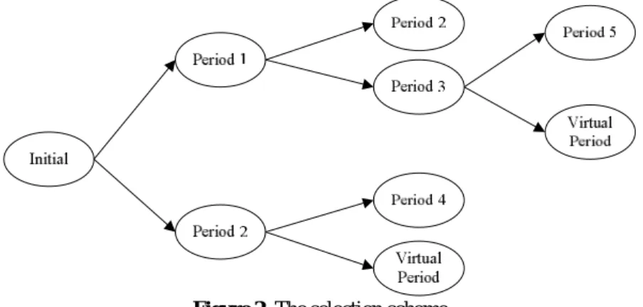
The condition for the termination of a route travelled by an ant is not the meeting of a certain number of nodes, but the meeting of two particular nodes, namely the node related to the last period in the planning horizon and a virtual node which indicates the termination of the route. The virtual node by which if it’s selected, the route termination condition will be satisfied, indicates that the production can be stopped in a period other than the last period and that the ant can directly enter the virtual node from the node corresponding to that period and satisfy the route termination condition. The initial node that an ant encounters along the route is a function of the first period in which there is a demand. In other words, if a demand emerges right in the first period, in order to not encounter shortage, the ants should choose node number (1) as the initial node of their movement route; and if a demand emerges in the second period, the ants should choose the initial node of their movement route from node number (1) or node number (2). This will be explained with the following example. Suppose that our planning horizon is finite and has four periods and in the second period we encounter demand for the first time. So our graph consists of nodes labeled 0 to 5; with node number 5 being the virtual node. The ant chooses the first, third and fifth nodes and completes its route. The selection schemes for the above example, from the beginning to the end of the route, can be seen in Figure 2.
Figure 2. The selection scheme
As Figure 2 shows, in the first, second and third moves, there are 2, 4 and 2 selection cases, respectively. At every step that period 4 or 5 is chosen the ant’s movement stops.
Following the completion of a route for a product, the value of variable becomes one, for the selected periods and zero for the other periods. However, since our problem is a multi-product problem, the movement route of an ant is not completed with the completion of the sequence of the product’s production periods, and upon the completion of this sequence, it is time to determine the production periods of products at lower levels.
Since the product’s number increases from the highest level (final product or products) toward the lowest level the ant also starts its route from product number 1 and proceeds to
the product with the highest number. In other words, after determining the production period sequence of the first product, the production period sequence of the second one and then the third one is determined and this procedure continues until the production period sequences of all the products are determined. To prevent shortage in the system, an ascending order of selecting product numbers has been adopted in the ant’s movement route, because the selection of the first production period of a product depends on the first production period of product or products at a higher level than that product, which indicates the internal demand for that product.
j
S
set of products in the production network, for which, product i is a prerequisite.j
k
the number of the first period in which product j, (j S ) j is manufactured. i
m the number of the first period in which product i has external demands. { j; j}
K Min k jS { i, }
M Min m K
The first to periods are the candidate periods for the first production period of product i.
3.2. Determination of variable
The value of variable , which equals the amount of production of product i during period t, is a function of the values of the variable associated with the production startup (Yit,t 1,...,T) and considering the values of . It can be determined as follows:
For each product i in every period t, if
Y
it
0
, thenX
it
0
For each product i in periods
t
1
t
2
T
, if Yi,t1 Yi,t2 1 and relation Yit 0 isestablished for each period t where
t
1
t
t
2, then we have: 21
1 j
t -1
i,t i,t i,j j,t
t=t jÎS
X =
(d +
r X ) (6)In the above relation, it is observed that the amount of production of every product i in period
t
1 equals the sum of all external and internal demands for product i from periodt
1 to periodt
2
1
.3.3. Probability function of choosing a movement route
The probability function of selecting a movement route depends on the existing pheromone concentration in the route and also on the heuristic information associated with route attractiveness and the parameters of
and
.The probability of selecting the route from m to n (n
U), such as going from period m to n for product i, ispi(m,n), which is expressed by equation (7):, ,
[
(
, )] .[
(
, )]
(
, )
[
(
, )] .[
(
, )]
i k i
i
i k i
n U
m n
m n
p m n
m n
m n
where i,k(m,n) is the existing pheromone concentration in the route from m to n for product i, in the kth step, i(m,n) is the heuristic function indicating the attractiveness of choosing the route from m to n for product i. U is the set of nodes that have been situated after node m in the movement route graph and
and
are the parameter of intensifying the effect of pheromone concentration and route attractiveness, respectively, whose value are determined with respect to problem conditions3.4. Fitness function of the solution
If the obtained solution is feasible, then the fitness function of the obtained solution (s) will be equal to the sum of the system costs, including the holding cost, startup cost and the cost of production.
1 1
( )
(
)
N T
it it it it it it i t
fit
value s
s Y
c X
h I
(8)If the output of the proposed method still has an infeasible solution, after the implementation of the carry-over rule, then the fitness function corresponding to that solution will not be calculated.
3.5. Determining the pheromone intensity parameter
The value of parameter i(m,n), which indicates the concentration of pheromone on the crest from m to n for product i, depends on the amount of initial pheromone (0) and the fitness function value; and considering the solutions obtained at each step, it is updated as follows:
If the obtained solution is infeasible and the capacity constraint has been disregarded in it, then the pheromone concentration associated with the existing nodes in the traversed path will not be updated.
, 1
(
, )
,(
, )
i k
m n
i km n
(9) If the obtained solution is feasible, then the pheromone concentration of the existing nodes in the traversed path will be updated according to equation (10):
, 1
(
, )
,(
, )
,(
, )
i k
m n
i km n
i km n
(10)where k(m,n) indicates the quality of the obtained solution (s) and can be computed by Eq. (11):
i ,k
W ( m ,n )
fit value ( s )
(11)
where W is a constant value, which is determined based on the characteristics of the problem.
3.6. Determining the route attractiveness parameter
The route attractiveness parameter (i) is a heuristic parameter which, not only provides the proper route selection conditions, but also establishes a balance between the two categories of search. This parameter consists of two parts associated with the setup cost and the holding cost. Equation (12) shows the heuristic route attractiveness parameter of a path from m to n for product i:
, ,
1
(
, )
(
, )
(
, )
i
i h i a
m n
m n
m n
(12) if 1 , , ,(
)
0
j
n
i t i j j t
t m j S
d
r X
then 1 1, , , , 1 , , , ,
, 1 , , ,
.
((
(
)
(
)).
)
(
, )
(
)
j j jn n l
i t i j j t i m i t i j j t i l
l m t m j S t m j S
i h n
i t i j j t
t m j S
B
d
r X
I
d
r X
h
m n
d
r X
and 1 , , , 1 1 , , 1.(
).
2
(
, )
(
).
T n m
i t i m t i n
t m t
i a T
i t i t m
B
s
s
s
m n
s
D
where B is a constant value which is defined with respect to the problem, Di is the internal and external average demand of product i.
The value of parameter , ( , ), which is related to the holding cost, indicates the
ratio of the holding cost incurred by the system to the amount of fulfilled demand due to the selection of period n after period m. Thus, the numerator of relation , ( , ) includes the
holding cost of selecting node n multiplied by the constant number B and the denominator of this ratio includes the amount of fulfilled demand as a result of choosing node n. To calculate , ( , ) at every route selection step of product i, the holding cost for each
choice should be estimated with respect to the search results of products above the level of product i and also with respect to the choice of periods smaller than period m in the production periods of product i. This increases the run time of the program to some extent, but this kind of computing the heuristic information associated with route attractiveness will enjoy a higher accuracy and therefore, a better solution quality.
Parameter , ( , ), which is corresponded to the setup cost, tends to pay a lower setup
cost and produce more of product i in a less number of production periods. 3.7. Global update of pheromone intensity
In each iteration of the algorithm solution, the pheromone intensity for the arrows forming the best found routes up to that stage of algorithm solution should be updated according to equation (13):
, ( , ) , ( , ) ( , )
i k m n i k m n k m n
(13)
where ( , )
( )
k
W m n
fit value best solution
.
3.8. Evaporation
In order to prevent premature convergence, in each iteration of the algorithm, some of the pheromone intensity in a route evaporates, before the route is constructed. At every step, the pheromone intensity is reduced by a constant rate called the rate of pheromone evaporation (
). The value of
is between 0 and 1 and it is a search history control parameter, which for a higher value of it, the attention to the past becomes weaker and the search takes on a more random and chance disposition. The evaporation can be calculated by equation (14):, ( , ) (1 ) , ( , )
i k m n i k m n
(14)
3.9. Number of ants
The number of ants is one of the effective parameters of the algorithm and we take it to be equal to the number of periods in the planning horizon.
3.10. The shifting technique
In this section, an important part of the algorithm called the shifting technique is described. After determining the production periods and specifying the values of variable by the ant colony algorithm, it is time to apply the shifting technique. At this step, the procedures for the calculation of variable , after determining the values of variable , are explained.
For each product i in each period t, if
Y
it
0
, thenX
it
0
For each product i in periods
t
1
t
2
T
, if Yi,t1 Yi,t2 1 and relation Yit 0 is established for every period t wheret
1
t
t
2, then we have:2 1
1
1
,
(
, , ,)
j
t
i t i t i j j t
t t j S
X
d
r X
(15)Equation (16) indicates that the amount of production of every product in period , equals the sum of the external and internal demands of product i from period to period −1. The obvious point in this relation is the lack of considering capacity constraint in the calculation of variable . So, to take this matter into consideration, the carry-over rule will be used. In this rule, the following steps shall be implemented:
Step (1): We move from period T toward period 1 and calculate the capacity index (qkt) for all the production resources, as follows:
1
(
.
. )
1, 2,...,
N
kt kit it kit it
i
CN
a
X
A Y
k
K
1, 2,..., kt
kt kt CN
q k K
C
(17)
Step (2): If all the values of qkt are smaller than or equal to 1, this means that capacity constraint has been considered in all the periods, so we proceed to step 8; otherwise we go step 3.
Step (3): If the value of qkt in period t and for resource k, is larger than 1, therefore according to the relation below, the amount of CRkt is smaller than zero.
0 1, 2, ...,
kt kt kt
CR C CN k K (18)
Step (3-1): If
t
1
, we stop (the problem’s solution is infeasible).Step (3-2): if
t
1
, the production amounts are carried over from period t to periodt
1
in order to establish the capacity constraint of resource k.The order of the product’s’ carry-over is from products at lower levels to products at higher levels. This is for the fulfillment of production prerequisite and for not running into shortage. Also the carry-over order in terms of production resources starts from resource k with the highest qkt.
Prior to the carry-over, all the candidate products for such a transfer are specified, so we start from the lowest production level (L) and consider the relevant products of that level. Now, if product i of the considered level has uses resource k in period t, it will be entered into the list of candidates.
Step (4): For all the member products on the list of candidates, the amounts of shifting from period t to period t1 are calculated according to the following sub steps:
Step (4-1): For product i, if CRkt akit Xit0, then part of the production of i in period t is carried over to period t1. This value is equal to (
kit kt
a
CR
). Because of this shifting, we have:
kt kt
i,t-1 i,t-1 i,t i,t kt i,t-1
kit kit
CR CR
X =X - X =X + CR =0 Y =1
a a (19)
Step (4-2): For product i, if CRkt akit Xit0, then the whole production of i in period t is carried over to period
t
1
. Due to this shifting, we have:i,t i,t-1 i,t-1 i,t
i,t-1 i,t kt kt kit kit it
X =0 X
=X
+X
Step (5): We calculate the cost of carry-over for each candidate member of level L. This cost includes the costs of production, holding and startup, which have been imposed on the system because of the carry-over of product i.
Step (5-1): In the case that was described in step (4-1), if the value of Xi,t1 before the carry-over is larger than zero, the startup cost imposed on the system due to the carry-over (SCi) is equal to
SC
i
0
, otherwise SCi si,t1.The holding cost imposed on the system due to the carry-over (HCi) and the production cost imposed on the system because of the carry-over (PCi) can be computed by equation (21) and (22), respectively:
) . ( ) . ( ) ( 1 , 1 .
i p j t j j t i kit kti h O h
a CR HC (21) ) ) ( . ( )) ( . ( ) ( , 1 , , 1 ,
i p j t j t j j t i t i kit kti c c O c c
a CR
PC (22)
Step (5-2): In the case that was described in step (4-2), if the value of Xi,t1 before the carry-over is larger than zero, the startup cost imposed on the system due to the carry-over (
i
SC ) is SCi si t, , otherwise SCi si t,1sit.
The holding and the production costs imposed on the system because of the carry-over can be calculated by equation (23) and (24), respectively:
) . ( ) . ( ) ( 1 , 1 .
i p j t j j t i iti X h O h
HC (23) ) ) ( . ( )) ( . ( ) ( , 1 , , 1 ,
i p j t j t j j t i t i iti X c c O c c
PC
(24)
where
p
(
i
)
is the set of products in the production network which immediately precedes product I, Oj indicates part of product j,(
j
p
(
i
))
, which we have to shift from period t to periodt
1
to fulfill the prerequisite conditions due to the shifting of product i from period t to period t1.Step (5-3): The total cost imposed on the system because of the shifting of product i is equal to:
i i i
i SC HC PC
TSC (25)
This cost can be a positive or a negative number.
Step (6): Product i belonging to the candidates list of level L is selected for shifting with the following probability:
|
|
( )
|
|
i i
j j Candidate list
TCS
TCS
PR i
TCS
(26)If product i is selected, it will be removed from the list of candidates. Step (7): If qkt was still larger than 1:
Step (7-1): If the candidates list of level L is not empty, we go back to step (6).
Step (7-2): If the candidates list of level L is empty, we go to a higher level (L L 1) and return to step (3), otherwise, we go back to step (1).
Step (8): The amount of inventory at the end of the period is calculated based equation (27).
, , 1 , ,
1
j
i t i t i t j t
j s
I
I
X
X
t
T
(27)At the end of the shifting technique, the fitness function value of the obtained solution (if feasible) is determined.
4. The results
In this section, an example has been solved by the proposed method and its results have been compared with the results obtained through the three metaheuristic methods of SA (Kuik et al., 1993), TS (Kuik et al., 1993) and GA (Xie and Dong, 2002) and through the exact method of Lagrangian relaxation (LR) (Billington, McClain and Thomas, 1986). 4.1. Numerical example
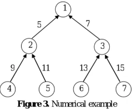
The production network has the following form, consisting of 7 (
N
7
) products in 3 levels.7 5
15 13
11 9
1
2 3
4 5 6 7
Figure 3. Numerical example
The length of the planning horizon (number of periods) is 6 (
T
6
) and the number of production resources is one (K 1).The information related to quantity of demand, available capacity of production resource, costs of startup and holding can be found in Tables 1 and Table 2, respectively.
Table 1. Demand and available capacity
6 5 4 3 2 4 Period t
10 90 0 100 0 40 External demand dit
1000 1000 5000 5000 0 10000 Available capacity Ct
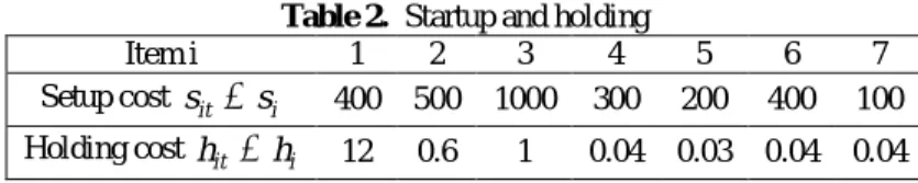
Table 2. Startup and holding 7 6 5 4 3 2 1 Item i 100 400 200 300 1000 500 400 Setup cost sit si
0.04 0.04 0.03 0.04 1 0.6 12 Holding cost hit hi
The production cost (cit) for every product, in every period is zero. )
, (
0 i t
cit We also have:
) , (
0 i t
Ait
2, 2 3, 3
0 , 2 , 3 5 , 8
it t t
a t i a a a a
4.2. Results analysis and comparisons
To analysis the performance and efficiency of the proposed hybrid method, we compare the mentioned example’s results with several well-known algorithms including simulated annealing (SA), tabu search (TS) and genetic algorithm (GA). All parameters of GA, SA, TS and HACO are reported in table 3.
Table 3. Range of algorithms parameters
Algorithm Parameter Value
GA
Population Size
Maximum Number of Generations Probability of Crossover Probability of Mutations
25 100 0.8 0.3 TS Neighborhood structure Maximum size of tabu list
Number of Iteration
3 10 100 SA Initial Temperature Final Temperature Cooling Ratio Number of iterations at a given
temperature 400 5 0.95 30 HACO α β W B Г
Number of iteration
2 1.25 100 20 2 0.01 100
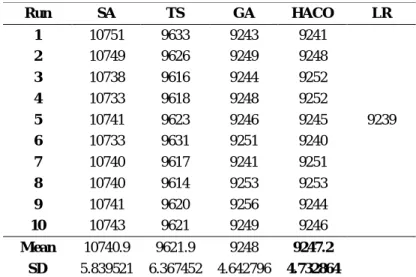
The problem was solved by running the proposed method and the four above-mentioned methods for ten times, giving the results in table 4.
Table 4. The computational results of solving the example
Run SA TS GA HACO LR
1 10751 9633 9243 9241 2 10749 9626 9249 9248 3 10738 9616 9244 9252 4 10733 9618 9248 9252
5 10741 9623 9246 9245 9239
6 10733 9631 9251 9240 7 10740 9617 9241 9251 8 10740 9614 9253 9253 9 10741 9620 9256 9244 10 10743 9621 9249 9246
Mean 10740.9 9621.9 9248 9247.2 SD 5.839521 6.367452 4.642796 4.732864
Figure 4 represented the graphical analysis of the results reported in Table 3. With regards to the mean and standard deviation (SD) metrics, SA and TS have significant difference with GA and proposed HACO. In order to do so, we plotted GA and HACO in comparison with exact solution of LR method in Figure 4. Moreover, according to the mean and SD values, HACO had a good performance rather than SA, TS, and GA.
Figure 4. Graphical comparisons of GA, HACO, and LR
6. Conclusion
In this study, the problem of economical determination of lot size in production systems with constrained capacity of production resources was investigated. The problem is NP-hard. A combination of the ant colony algorithm and a heuristic method called the carry-over rule was proposed for solving the problem. Then, by presenting an example, the results of the proposed method were compared with those of the other algorithms used by other researchers. Through these comparisons it was observed that the proposed method has adequate performance relative to other heuristic methods, such that, in comparison with the simulated annealing and tabu search methods, it has performed better and compared to the genetic algorithm, it has provided similar results. Of course, with the increase of the problem size and the extension of the search space, the effectiveness of the algorithm falters to some extent, which for improving the solution quality of large size problems, further development and enhancement of the presented algorithm through future studies has been contemplated. Furthermore, the development of the algorithm for the purpose of
9238 9243 9248 9253
1 2 3 4 5 6 7 8 9 10
GA HACO LR
solving problems that have carry-over setups (capable of being carried over) and also fuzzy demands can provide an appropriate groundwork for the continuation of research on this subject.
References
Absi N., Detienne B., Dauzere S. (2013), Heuristics for the multi-item capacitated lot-sizing problem with lost sales; Computers & Operations Research 40; 264-272. Absi N., Kedad-Sidhoum S. (2008), The multi-item capacitated lot-sizing problem with setup times and shortage costs; European Journal of Operational Research 185; 1351-1374.
Afentakis P., Gavish B., Karmarkar V. (1984), Optimal solutions to the lot-sizing problem in multi-stage assembly systems; Management Science 30; 222-239. Afentakis P., Gavish B. (1986), Optimal lot-sizing algorithms for complex product structures; Operations Research 34; 237-249.
Aggarwal A., Park J.K. (1993), Improved algorithms for economic lot size problems; Operations Research, 41; 549-571.
Aksen D., Altınkemer K., Chand S. (2003), The single-item lot-sizing problem with immediate lost sales; European Journal of Operational Research 147(3); 558-566. Almeder C. (2010), A hybrid optimization approach for multi-level capacitated lot-sizing problems; European Journal of Operational Research 200; 599-606.
Barang I., VanRoy T.J., Wolsey L.A. (1984), Strong formulations for multi item capacitated lot-sizing; Management Science 30; 1255-1261.
Belvaux G., Wolsey L.A. (2000), A specialized branch-and-cut system for lot-sizing problems; Management Science 46 (5); 724-738.
Billington P.J., McClain J.O., Thomas L.J. (1986), Heuristic for multi-level lot-sizing with a bottleneck; Management Science 32; 989-1006.
Brahimi N., Dauzere S. (2006), Review Single item lot-sizing problems; European Journal of Operational Research 168; 1-16.
Choi S., Enns S.T. (2004), Multi-product capacity-constrained lot sizing with economic objectives; International Journal of Production Economics 91(1); 47-62. Dellaert N., Jeunet J., Jonard N. (2000), A genetic algorithm to solve the general multi-level lot-sizing problem with time varying costs; International Journal of Production Economics 68; 241-257.
Friedman M., Winter J.L. (1978), A Study of the infinite horizon ‘solution’ of inventory lot size models with a linear demand function; Computers & Operations
Research 5(2); 157-160.
Gallego G., Shaw D.X. (1997), Complexity of the ELSP with general cyclic schedules; IEEE Transactions 29; 109–13.
Ganas I., Papachristos S. (2005), The single-product lot-sizing problem with constant parameters and backlogging; Exact results, a new solution, and all parameter stability regions; Operations Research 53 (1); 170–176.
Guan Y., Ahmed S., Miller AJ, Nemhauser G.L. (2006), On formulations of the stochastic uncapacitated lot-sizing problem; Operations Research Letters 34(3); 241-250.
Gupta Y.P., Keung Y. (1990), A review of multi-stage lot-sizing models; International Journal of Operations and Production Management 10; 57-73.
Gupta D., Magnusson T. (2005), The capacitated lot-sizing and scheduling problem with sequence-dependent setup costs and setup times; Computers & Operations Research 32 (4); 727-747.
Huang K., Küçükyavuz S. (2008), On stochastic lot-sizing problems with random lead times; Operations Research Letters 36(3); 303-308
Jans R., Degraeve Z. (2004), Improved lower bounds for the capacitated lot-sizing problem with setup times; Operations Research Letters 32; 185-195.
Jans R., Degraeve Z. (2007), Meta-heuristics for dynamic lot-sizing; A review and comparison of solution approaches; European Journal of Operational Research 177; 1855-1875.
Karimi B., Fatemi Ghomi S.M.T., Wilson JM. (2003), The capacitated lot-sizing problem; a review of models and algorithms; Omega 31; 365-378.
Kovacs A., Brown K.N., Tarim S.A. (2009), An efficient MIP model for the capacitated lot-sizing and scheduling problem with sequence-dependent setups; International Journal of Production Economics 118(1); 282-291.
Kuik R., Salomon M., Van Wassenhove L.N., Maes J. (1993), Linear programming, simulated annealing and tabu search heuristic for lot-sizing in bottleneck Assembly systems; IIE Transactions 25; 62-72.
Lambrecht M.R., VanderEchen J., VanderVeken H. (1981), Review of optimal and heuristic models for a class of facilities in series dynamic lot size problems, In Multi-Level Production-Inventory Control Systems; Theory and Practice, North-Holland, Amsterdam, 69-94.
Maes J., McClain J., VanWassenhove N .( 1991), Multilevel capacitated lot-sizing complexity and LP-based heuristics; European Journal of Operational Research 53 (2); 131-148.
MATLAB Version 7.10.0.499 (R2010a). The MathWorks, Inc. Protected by U.S. and international patents, 2010.
Ozdamar L., Barbarosoglu G. (2000), An integrated Lagrangian relaxation-simulated annealing approach to the multilevel multi-item capacitated lot-sizing problem; International Journal of Production Economics 68 (3); 319-331.
Pitakaso R., Almeder C., Doerner K., Hartl R. (2006), Combining population-based and exact methods for multi-level capacitated lot-sizing problems; International Journal of Production Research 44 (22); 4755-4771.
Pitakaso R., Almederb C., Doernerb K.F., Hartlb R.F. (2007), A MAX-MIN ant system for unconstrained multi-level lot-sizing problems; Computers & Operations Research 34; 2533-2552.
Rezaei J., Davoodi M. (2011), Multi-objective models for lot-sizing with supplier selection, International Journal of Production Economics 130(1); 77-86.
Robinson P., Narayanan A., Sahin F. (2009), Coordinated deterministic dynamic demand lot-sizing problem; A review of models and algorithms; Omega 37(1); 3-15.
Senyigit E., Düğenci M., Aydin M.E., Zeydan M. (2013), Heuristic-based neural networks for stochastic dynamic lot sizing problem; Applied Soft Computing 13( 3); 1332-1339.
Shim I.S., Kim H.C., Doh H.H., Lee D.H. (2011), A two-stage heuristic for single machine capacitated lot-sizing and scheduling with sequence-dependent setup costs; Computers & Industrial Engineering 61(4); 920-929.
Tempelmeier H., Derstroff M. (1996), A Lagrangean-based heuristic for dynamic multilevel multi item constrained lotsizing with setup times; Management Science 42 (5); 738-757.
Teng J.T., Chern M.S., Yang H.L., Wang Y.J. (1999), Deterministic lot-size inventory models with shortages and deterioration for fluctuating demand; Operations Research Letters 24; 65-72.
Toledo C.F.M., Ribeirode Oliveira R.R.R., Franca P.M. (2013), A hybrid multi-population genetic algorithm applied to solve the multi-level capacitated lot-sizing problem with backlogging; Computers & Operations Research 40; 910-919.
Ustun O., Demırtas E.A. (2008), An integrated multi-objective decision-making process for multi-period lot-sizing with supplier selection; Omega, 36(4); 509-521. Wolsey L.A. (1995), Progress with single-item lot-sizing; European Journal of Operational Research 86; 395-401.
Wua T., Shi L., Geunes J., Akartunalı K. (2011), An optimization framework for
Journal of Operational Research 214; 428-441.
Xiao Y., Kaku I., Zhao Q., Zhang R. (2011), A reduced variable neighborhood search algorithm for uncapacitated multilevel lot-sizing problems; European Journal of Operational Research 214; 223-231.
Xie J., Dong J. (2002), Heuristic Genetic Algorithms for General Capacitated Lot-Sizing; An International journal computers & mathematics 44; 263-276.
Zhou Y.W., Lau H.S., Yang S.L. (2004), A finite horizon lot-sizing problem with time-varying deterministic demand and waiting-time-dependent partial backlogging; International Journal of Production Economics 91(2); 109-119.