Vol. 2, No. 4, pp 288-296 Winter 2009
Fast Generation of Deviates for Order Statistics by an Exact Method
Hashem Mahlooji1*, Hossein Abouee Mehrizi2, Azin Farzan31Sharif University of Technology, Iran; 1 [email protected]
2The University of Toronto, Ontario, Canada, 3
University of Washington, Seatle, WA, USA
ABSTRACT
We propose an exact method for generating random deviates from continuous order statistics. This versatile method that generates Beta deviates as a middle step can be applied to any density function without resorting to numerical inversion. We also conduct an exhaustive investigation to document the merits of our method in generating deviates from any Beta distribution.
Keywords: Order Statistics, Beta Variate, Exact Method, Rejection Method, Equal Probability Partition.
1. INTRODUCTION
There exist numerous applications in which practitioners need to study the behavior of a stochastic system by means of generating order statistics. The problems in the field of reliability engineering generally deal with order statistics. The proposed methods for generating deviates from order statistics (OS) fall in two categories: those which resort to generating Beta deviates as a middle step and those which do not. Several methods have been proposed for generating order statistics each of which has its own advantages as well as drawbacks. These methods range from the common sense (NAÏVE) method which simulates all order statistics to the elegant Transformed Density Rejection
(TDR) method proposed by Hormann and Derflinger (2002) and the Uniform Fractional Parts
(UFP) recently developed by Mahlooji et al (2008). A well known method for generating order statistics stems from the properties of the Inverse Transform method whenever applicable. Devroye (1980) proposed the Quick Elimination (QE) method which works faster than the NAÏVE method. This method still needs to generate part of the series of random variables and is capable of generating deviates for the minimum and the maximum only. Even though the UFP method works very fast, it suffers from its non-exact nature that leads to generating biased samples when the sample size is very large. So at the cost of losing some speed, we modify this method to make it an exact method which is completely free of biased sampling.
*
Since our proposed method falls in the category of the so called inversion methods, a significant part of it consists of generating random deviates from Beta density function. Due to the flexibility
of the shape of Beta distribution in response to the variations in its parameters a and b, a number of
methods have been proposed to generate Beta deviates. Johnk (1964) proposed the first algorithm
for generating Beta deviates for any values of a and b. Ahrens and Dieter (1974 a and b) proposed
the BN method which has a slow performance. The switch method was developed by Atkinson and
Whittaker (1976) which was specifically designed for the case of a, b>1. Later, Atkinson (1979)
generalized this method to any value of a and b even through his proposed method was
outperformed by Johnk’s method when a + b<1. Cheng (1978) proposed a simple method for any
values of a and b. Schmiser and Babu (1980) proposed an efficient method for the case of a, b >1
based on the rejection method (B4PE). Later, Sakasegawa (1983) proposed his stratified rejection method for generating Beta deviates. Zechner and Stadlober (1992) proposed the patchwork rejection method which was faster than some of the existing methods at the time but suffered from the long setup time (BPRB and BPRS). Hormann, Leydold and Derflinger (2004) proposed the Transformed Density Rejection (TDR) method which is rather complicated. Numerical inversion methods in generating random deviates date back to 1983 (Devroye, 1986). The latest in this category was proposed by Hormann and Leydold (2003). All the algorithms falling in this category are in need of the Beta CDF and resort to an approximation in treatment of the problem.
Mahlooji, et al. (2005)proposed UFP as a non-exact method for generating random deviates for any
of the order statistics where sample is taken from a continuous random variable. Since their algorithm does not require any search algorithm (like index search), it outperforms methods like TDR when it comes to speed of computation and simplicity. Like TDR, UFP is in need of the break (grid) points during the set up step. As stated, this method runs into rather serious problems in generating large samples free of bias. So we show how to modify UFP in order to make it work as an exact method. Our modified algorithm still is short even though it loses some speed. At the heart
of the revised method lies the necessity of generating deviates from Beta (a, b) for a,b≥1. We
therefore will do an in depth evaluation on the capability of this method in generating deviates from any Beta density function and then address the issue of generating random deviates for the order statistics.
2. THEORITICAL BASIS OF THE ALGORITHM
Since the algorithm developed in this work is the exact version of the UFP method, we briefly introduce the theoretical basis of UFP including the relevant algorithms. The following theorem provides the basis for UFP.
Theorem
Given continuous independent random variables U1~U
[ ]
0,1 andX, then the random variable[
U X]
XU
U2 = 1+ − 1+ is distributed as a U [0, 1].
We can obviously write
[
U X]
X U
U2 = 1+ − 1+ (1)
⎣
U X⎦
U U
X = 2− 1 + 1+ (2)
or
⎣ ⎦
X U1 U2 I[
U1 U2]
X = + − + < (3)
where, I
[
U1<U2]
is an indicator function.It can easily be established that U1−U2+I
[
U1 <U2]
behaves as a U [0, 1] random variable when1
U and U2are independent. Thus under such circumstances (3) simplifies to
⎣ ⎦
X U, U ~U(0,1)X = + (4)
As far as relation (4) is concerned, the grid points consist of some integer values on the X-axis. To
generalize the conditions such that any n distinct real values ai in the range of X can form the grid
points, we adopt the approach that forms a uniform probability partition of the range of the random variable X. That is, for the grid points a1,…an, the relation
... ) ( ) ( ... ) ( ) ( ) ( ) ( )
(a1 =F a2 −F a1 =F a3 −F a2 = =F ai −F ai−1 =
F (5)
holds and (5) can be rewritable as
i i i
i U d a a
d X Int
X = ( )+ * , = +1 − (6)
where, di=ai+1-ai , i=0, 1, 2…n and
(
)
⎩ ⎨ ⎧ > • + < • + = • + + + + 1 1 1 , , i i i i a X a a X a XInt (7)
This approach leads to a partition of the range of X into a number of segments where the probability
associated with each segment is equal to p=1/n.
The following algorithm can be applied to the density of any continuous random variable including Beta (a, b).
Algorithm 1 (UFP)
1) Determine the value of partition size p, and define the grid points a1,…an and the di values.
2) Generate a random numberU'.
3) Set ⎥
⎦ ⎥ ⎢ ⎣ ⎢ + p U'
4) Determine Int(X)=ai on the basis of i.
5) Generate a random number U.
6) DeliverX =Udi +ai.
The following algorithm can generate order statistics.
Algorithm 2 (OSUFP)
1) Determine the values of the parameters of the Beta distribution on the basis of the jth order
statistics a = j and b= n – j + 1.
2) Generate a random deviate from Beta (a, b) based on the Algorithm 1 and designate it by β.
3) Determine the partition size p and define the grid points a1…an anddi values for the intended
distribution for which order statistics are to be generated.
4) Set ⎥
⎦ ⎥ ⎢ ⎣ ⎢ +
p
β
1 equal to i where p stands for the partition size.
5) Determine Int(X)=ai on the basis of i.
6) Generate a random number U.
7) DeliverX =Udi +ai.
3. MODIFYING THE UFP ALGORITHM
The main idea in converting the UFP algorithm to an exact method is to implement the rejection
method over each interval
[
ai,ai+1)
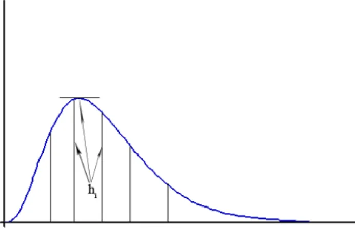
, i=1,2,",n−1in such a way that the enveloping functionover each interval, hi, is defined as a U[ai,ai+1] (See Figure 1).
In Figure 1, hiis defined as
} :
) (
{ ≤ < +1
= i i
i Sup f x a x a
h (8)
For instance, when the density function f(x)is monotonically decreasing over the interval
[
ai,ai+1)
we have hi = f(ai). In case f(x)is monotonically increasing over that interval theni
h assume a value equal to f(ai+1).
In this way, there are a maximum of n−1different uniform enveloping functions each of which is
defined over one of the intervals
[
ai,ai+1)
, i=1,2,",n−1. Once implemented, the rejectionmethod operates in its usual manner which means that a number of generated points will be discarded. The experimental results, however, agree with the expectation that the combination of UFP and the rejection method will drastically reduce the number of rejected points and hence increase the efficiency of this exact algorithm. Table 1 shows that as the number of intervals in the
range of X increases, the number of rejections tends to zero when f(x) is distributed as a negative
experimental distribution. This behavior can be expected regardless of the distribution of the
continuous random variableX .
At this point we present the modified algorithms in its final form. Algorithm 3 is an exact algorithm intended to generate values for any Beta distribution, while Algorithm 4 is the exact version of algorithm 2 and is intended to generate a deviate for the given order statistic. Step 2 in this algorithm takes the output of the Algorithm 3 as an input.
Algorithm 3 (UFPExact)
1) Determine the value of partition size p, and define the grid points a1,…an and the di values
2) Generate a random numberU'.
3) Set ⎥
⎦ ⎥ ⎢ ⎣ ⎢
+
p
U'
1 equal to I ,determine Int(X)=ai, and hi =Sup{f(x):ai ≤x<ai+1}
4) Generate a random number U.
5) SetX =Udi +ai.
6) Generate the uniform deviate Y over the interval
[ ]
0,hi .7) Accept X as defined in step 5 (and go to Algorithm 4) iff(x)≤Y; otherwise, reject it and
go to step 2.
Algorithm 4 (OSUFPExact)
1) Depending on the intended value of the jth order statistic, determine the parameter value of the
relevant Beta distribution as a= jandb=n− j+1.
3) Determine the partition size, p; the grid points, a1,…an; and d1,…,dn-1 for the intended
density function for which order statistics are to be generated.
4) Set ⎥
⎦ ⎥ ⎢ ⎣ ⎢ +
p
β
1 equal to i, determine Int(X)=ai, and hi =Sup{f(x):ai ≤x<ai+1}
5) Generate a random number U.
6) SetX =Udi +ai.
7) Generate the uniform deviate Y over the interval
[ ]
0,hi .8) Accept X(step 6) as a random variate for the intended order statistic if f(x)≤Y holds;
otherwise, rejectX and return to step 2.
It is obvious that Algorithms 3 and 4 are basically one in nature. The only difference between them
is the way that f(x) is defined in each algorithm. While f(x) in Algorithm 3 is always defined as
a Beta
[
j,n− j+1]
for the same specified values of nand j, in Algorithm 4 f(x)represents adensity function whose jth order statistic needs to be sampled on computer.
4. EXPERIMENTAL RESULTS
This section presents the results of employing the modified algorithms to generate deviates for Beta random variables as well as the order statistics. In each case the performance of the relevant modified algorithm is compared against the most viable existing methods in terms of speed of
computation (
μ
s) and the degree of conformity (P-value in goodness of fit testing). To run theexperiments we wrote Java programs for each method and ran all programs on an AMD Attlon processor. The numerical results displayed in Tables 2 to 5 are the averages of 20 independent runs of 1000 deviates each.
Table 1 The number of accepted points as a function of the number of segments in the partition 1000 500
200 100
50 20
10 No. of Segments
99.8 99.4
97.9 97
95.5 90.2
81.8 Number accepted
Since we have combined the rejection method and the UFP algorithm to construct the exact UFP algorithm, we have studied the number of rejections when the number of segments in the partition tends to increase. Table 1 shows that the number of rejected points in the application of the exact algorithm developed in this work tends to zero as the number of partitions becomes larger. Under these circumstances the efficiency of the exact algorithm improves beyond the conventional standards of any purely rejection method.
In this work we have examined a quite broad range of values representing the number of segments
but only three values are included in Tables 2, 3 and 4 which are identified by p = 0.05, 0.02, and
0.01. In other words, we have defined partitions with 20, 50, and 100 segments of equal probability. UFP and UFPExact are the only methods among those listed in Tables 2 through 4 which are
We now present the numerical results of our experiments for Beta and order statistics separately.
I. Generating Beta random deviates.
Depending on the parameter values of the Beta distribution being at least 1 or less than 1, there exist different methods for generating Beta deviates for each case. Since our proposed method is among the algorithms that can be applied to both cases, we have studied its performance against its competitors both when the parameters of Beta are 1 or larger (Tables 2 and 3) and when they are smaller than 1 (Table 4). The outcome of the comparisons can be summarized as follows.
a) It can be asserted that regardless of the parameter values of Beta distribution, the speed of the
exact algorithm developed in this work (UFPExact) is constant in generating Beta deviates while some methods show varying speeds when the parameters of Beta distribution assume different values (See Tables 2, 3 and 4).
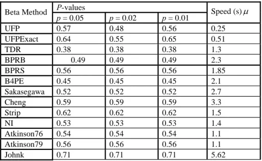
Table 2 Computing the performance of the exact UFP against 12 existing algorithms in generating
Beta deviates. (a =1.5, b = 2.2)
P-values
Beta Method
p = 0.05 p = 0.02 p = 0.01 Speed (s)
μ
UFP 0.57 0.48 0.56 0.25
UFPExact 0.64 0.55 0.65 0.51
TDR 0.38 0.38 0.38 1.3
BPRB 0.49 0.49 0.49 2.3
BPRS 0.56 0.56 0.56 1.85
B4PE 0.45 0.45 0.45 2.1
Sakasegawa 0.52 0.52 0.52 2.7
Cheng 0.59 0.59 0.59 3.3
Strip 0.62 0.62 0.62 1.5
NI 0.53 0.53 0.53 1.4
Atkinson76 0.54 0.54 0.54 1.1
Atkinson79 0.56 0.56 0.56 1.1
Johnk 0.71 0.71 0.71 5.62
b) Regardless of the number of segments in the partition, speed of the exact algorithm is
constant as shown in Tables 2, and 3.
c) Based on its biased performance in large samples, if we exclude the UFP method from
consideration, the exact algorithm developed in this work outperforms all the existing methods in terms of speed. In fact, as displayed in Tables 2, and 3, UFPExact is almost twice as fast as its closest competitor.
d) In terms of conformity of the generated samples, the proposed method shows a strong
performance too. The new algorithm leads to better P-values when compared to the
approximate UFP. This is due to the new method’s exact nature and is quite expected.
Among the remaining methods, we restrict our comparison to the case p = 0.01 where at
times UFPExact comes second to Johnk’s algorithm whose serious drawback is its very slow speed.
Table 3 Comparing the performance of the existing algorithms in generating Beta (a = 0.3,b = 0.7) deviates
P-values
Beta Method
p = 0.05 p = 0.02 p = 0.01 Speed (s)
μ
UFP 0.28 0.55 0.62 0.25
UFPExact 0.51 0.62 0.72 0.51
Strip 0.56 0.56 0.56 1.5
NI 0.52 0.52 0.52 1.4
Atkinson76 0.54 0.54 0.54 1.3
Atkinson79 0.56 0.56 0.56 1.3
Jonk 0.54 0.54 0.54 1.4
Table 4 Comparison of the speed of the exact UFP algorithm against other algorithms in generating deviates for order statistics
Order Statistics OS Method
1 200 500 1000
OSUFP 0.44 0.44 0.44 0.44
OSUFPExact 0.81 0.81 0.81 0.81
OSTDR 2.6 2.6 2.6 2.6
OSStrip 2.7 2.7 2.7 2.7
QE 9.4 - - 8.6
OSINV 2.1 2.1 2.1 2.1
NAIVE 443 443 443 443
II. Generating random deviates for the jth order statistic
To check the merits of our proposed method in generating deviates for order statistics, we assumed
) (x
f is defined as a Gamma density function with parameters 1.5 and 2.8. Table 4 displays the
speed of our proposed method in generating random deviates for the first, 200th, 500th, and 1000th
order statistics compared to other existing methods. As noted before, Quick Elimination (QE) method is just capable of. generating deviates for the minimum and the maximum in a sample. It can be seen that when not considering the approximate UFP, the exact algorithm developed in this study works 2.5 times faster than its nearest competitor.
5. CONCLUSION
In this work we introduced an exact method for the purpose of generating random deviates for order statistics which is based on the UFP and the Rejection methods. In order to come up with a definitive conclusion, we studied all the relevant methods in generating Beta deviates as well as methods designed for generating order statistics. Our findings indicate that the exact version of UFP outperforms all the existing methods in generating both Beta variates and order statistics except the approximate UFP. This still is considered as a breakthrough in the sense that the approximate UFP is at fault when it comes to generating large samples. The main advantage of the proposed method lies in its high speed of computations while the conformity of the generated samples to their intended distributions is very high.
REFERERENCES
[1] Ahrens J.H., Dieter U. (1974), Computer methods for sampling from gamma, beta, Poisson and binomial distributions; Computing 12; 233-246.
[2] Ahrens J.H., Dieter U. (1974), Acceptance-rejection techniques for sampling from the gamma and beta distributions; Technical Report 83; Stanford, California, Stanford University.
[3] Atkinson A.C., Whittaker J. (1976), A switching algorithm for the generation of beta random variables with at Least One Parameter less than 1; Journal of The Royal Statistical Society 139; 431-467.
[4] Atkinson A.C. (1979), A family of switching algorithms for computer generation of beta random variables; Biometrika 66; 141-145.
[5] Cheng R.C.H. (1978), Generating beta variates with nonintegral shape parameters; Comm. ACM 21; 317-322.
[6] Devroye L. (1980), Generating the maximum of independent identically distributed random variables; Comput. Math. Appl. 6; 305-315.
[7] Devroye L. (1986), Non-uniform random variate generation; Springer-Verlag.
[8] Hörmann W., Derflinger G. (2002), Fast generation of order statistics; ACM Transactions on Modeling and Computer Simulation 12(2); 83-93.
[9] Hörmann W., Leydold J., Derflinger G. (2004), Automatic nonuniform random variate generation; Sprigner-Verlag.
[10] Hörmann W., Leydold J. (2003), Continuous random variate generation by fast numerical inversion; ACM Trans. Model. Comput. Simul. 13(4); 347-362.
[11] Johnk M.D. (1964), Erzeugung von betaverteilten und gammaverteilten zufallszahlen; Metrika 8; 5-15. [12] Mahlooji H., Jahromi A. E., Mehrizi H. A., Izady N. (2008), Uniform fractional part: A simple fast
method for generating continuous random variates; Scientia Iranica 15(5); 613-622.
[13] Mahlooji H., Mehrizi H.A., Farzan A. (2005), A fast method for generating continuous order statistics based on uniform fractional parts; 35th International Conference on Computers and Industrial Engineering Turkey(Istanbul); 1355-1360.
[14] Sakasegawa H. (1983), Stratified rejection and squeeze method for generating beta random numbers; Ann. Inst. Statist. Math. 35; 291-302.
[15] Schmeiser B.W., Babu A.J.G. (1980), Beta variate generation via exponential majorizing functions; Oper. Research 28; 917-926.
[16] Zechner H., Stadlober E. (1992), Generating beta variates via patchwork rejection; Technical report; Institute for Statistik, Techn. University Graz.