2 The wireless channel

(1)

2

The wireless channel

A good understanding of the wireless channel, its key physical parameters and the modeling issues, lays the foundation for the rest of the book. This is the goal of this chapter.

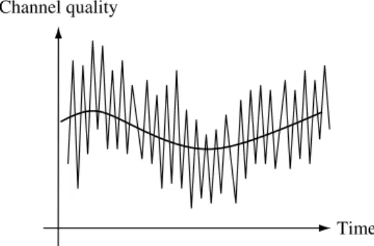
A defining characteristic of the mobile wireless channel is the variations of the channel strength over time and over frequency. The variations can be roughly divided into two types (Figure 2.1):

• Large-scale fading, due to path loss of signal as a function of distance and shadowing by large objects such as buildings and hills. This occurs as the mobile moves through a distance of the order of the cell size, and is typically frequency independent.

• Small-scale fading, due to the constructive and destructive interference of the multiple signal paths between the transmitter and receiver. This occurs at the spatial scale of the order of the carrier wavelength, and is frequency dependent.

We will talk about both types of fading in this chapter, but with more emphasis on the latter. Large-scale fading is more relevant to issues such as cell-site planning. Small-scale multipath fading is more relevant to the design of reliable and efficient communication systems – the focus of this book.

We start with the physical modeling of the wireless channel in terms of elec-tromagnetic waves. We then derive an input/output linear time-varying model for the channel, and define some important physical parameters. Finally, we introduce a few statistical models of the channel variation over time and over frequency.

2.1 Physical modeling for wireless channels

Wireless channels operate through electromagnetic radiation from the trans-mitter to the receiver. In principle, one could solve the electromagnetic field equations, in conjunction with the transmitted signal, to find the

(2)

11 2.1 Physical modeling for wireless channels

Figure 2.1Channel quality varies over multiple time-scales. At a slow scale, channel varies due to large-scale fading effects. At a fast scale, channel varies due to multipath effects.

Time Channel quality

electromagnetic field impinging on the receiver antenna. This would have to be done taking into account the obstructions caused by ground, buildings, vehicles, etc. in the vicinity of this electromagnetic wave.1

Cellular communication in the USA is limited by the Federal Commu-nication Commission (FCC), and by similar authorities in other countries, to one of three frequency bands, one around 0.9 GHz, one around 1.9 GHz, and one around 5.8 GHz. The wavelength of electromagnetic radiation at any given frequency f is given by =c/f, where c=3×108_{m/s is the}

speed of light. The wavelength in these cellular bands is thus a fraction of a meter, so to calculate the electromagnetic field at a receiver, the locations of the receiver and the obstructions would have to be known within sub-meter accuracies. The electromagnetic field equations are therefore too complex to solve, especially on the fly for mobile users. Thus, we have to ask what we really need to know about these channels, and what approximations might be reasonable.

One of the important questions is where to choose to place the base-stations, and what range of power levels are then necessary on the downlink and uplink channels. To some extent this question must be answered experimentally, but it certainly helps to have a sense of what types of phenomena to expect. Another major question is what types of modulation and detection techniques look promising. Here again, we need a sense of what types of phenomena to expect. To address this, we will construct stochastic models of the channel, assuming that different channel behaviors appear with different probabilities, and change over time (with specific stochastic properties). We will return to the question of why such stochastic models are appropriate, but for now we simply want to explore the gross characteristics of these channels. Let us start by looking at several over-idealized examples.

1 _{By obstructions, we mean not only objects in the line-of-sight between transmitter and} receiver, but also objects in locations that cause non-negligible changes in the electro-magnetic field at the receiver; we shall see examples of such obstructions later.

(3)

2.1.1 Free space, fixed transmit and receive antennas

First consider a fixed antenna radiating into free space. In the far field,2 _the

electric field and magnetic field at any given location are perpendicular both to each other and to the direction of propagation from the antenna. They are also proportional to each other, so it is sufficient to know only one of them ( just as in wired communication, where we view a signal as simply a voltage waveform or a current waveform). In response to a transmitted sinusoid cos 2ft, we can express the electric far field at timetas

Ef t r =s f cos 2ft−r/c

r (2.1)

Here,r represents the point u in space at which the electric field is being measured, wherer is the distance from the transmit antenna touand where represents the vertical and horizontal angles from the antenna tourespectively. The constantcis the speed of light, and_s f is the radiation pattern of the sending antenna at frequencyfin the direction ; it also contains a scaling factor to account for antenna losses. Note that the phase of the field varies withfr/c, corresponding to the delay caused by the radiation traveling at the speed of light.

We are not concerned here with actually finding the radiation pattern for any given antenna, but only with recognizing that antennas have radiation patterns, and that the free space far field behaves as above.

It is important to observe that, as the distancerincreases, the electric field decreases asr−1_{and thus the power per square meter in the free space wave}

decreases asr−2_{. This is expected, since if we look at concentric spheres of}

increasing radiusr around the antenna, the total power radiated through the sphere remains constant, but the surface area increases asr2_{. Thus, the power}

per unit area must decrease asr−2_{. We will see shortly that this}_r−2_reduction

of power with distance is often not valid when there are obstructions to free space propagation.

Next, suppose there is a fixed receive antenna at the locationu=r . The received waveform (in the absence of noise) in response to the above transmitted sinusoid is then

E_rf tu= f cos 2ft−r/c

r (2.2)

where fis the product of the antenna patterns of transmit and receive antennas in the given direction. Our approach to (2.2) is a bit odd since we started with the free space field atuin the absence of an antenna. Placing a

2 _{The far field is the field sufficiently far away from the antenna so that (2.1) is valid. For} cellular systems, it is a safe assumption that the receiver is in the far field.

(4)

receive antenna there changes the electric field in the vicinity ofu, but this is taken into account by the antenna pattern of the receive antenna.

Now suppose, for the givenu, that we define

Hf = f e

−j2fr/c

r (2.3)

We then have E_rf tu= Hf ej2ft_{. We have not mentioned it yet,}

but (2.1) and (2.2) are both linear in the input. That is, the received field (waveform) atu in response to a weighted sum of transmitted waveforms is simply the weighted sum of responses to those individual waveforms. Thus, Hf is the system function for an LTI (linear time-invariant) channel, and its inverse Fourier transform is the impulse response. The need for understanding electromagnetism is to determine what this system function is. We will find in what follows that linearity is a good assumption for all the wireless channels we consider, but that the time invariance does not hold when either the antennas or obstructions are in relative motion.

2.1.2 Free space, moving antenna

Next consider the fixed antenna and free space model above with a receive antenna that is moving with speedv in the direction of increasing distance from the transmit antenna. That is, we assume that the receive antenna is at a moving location described asut=rt withrt=r₀+vt. Using (2.1) to describe the free space electric field at the moving pointut(for the moment with no receive antenna), we have

Ef t r₀+vt =s f cos 2ft−r0/c−vt/c

r₀+vt (2.4) Note that we can rewrite ft−r₀/c−vt/c as f1−v/ct−fr₀/c. Thus, the sinusoid at frequency f has been converted to a sinusoid of frequency f1−v/c; there has been a Doppler shift of −fv/c due to the motion of the observation point.3 _{Intuitively, each successive crest in the transmitted}

sinusoid has to travel a little further before it gets observed at the moving observation point. If the antenna is now placed at ut, and the change of field due to the antenna presence is again represented by the receive antenna pattern, the received waveform, in analogy to (2.2), is

E_rf t r₀+vt = f cos 2f 1−v/ct−r0/c

r₀+vt (2.5) 3 _{The reader should be familiar with the Doppler shift associated with moving cars. When an}

ambulance is rapidly moving toward us we hear a higher frequency siren. When it passes us we hear a rapid shift toward a lower frequency.

(5)

This channel cannot be represented as an LTI channel. If we ignore the time-varying attenuation in the denominator of (2.5), however, we can represent the channel in terms of a system function followed by translating the frequencyf by the Doppler shift−fv/c. It is important to observe that the amount of shift depends on the frequencyf. We will come back to discussing the importance of this Doppler shift and of the time-varying attenuation after considering the next example.

The above analysis does not depend on whether it is the transmitter or the receiver (or both) that are moving. So long asrt is interpreted as the distance between the antennas (and the relative orientations of the antennas are constant), (2.4) and (2.5) are valid.

2.1.3 Reflecting wall, fixed antenna

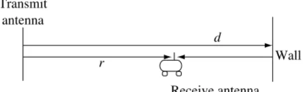
Consider Figure 2.2 in which there is a fixed antenna transmitting the sinusoid cos 2ft, a fixed receive antenna, and a single perfectly reflecting large fixed wall. We assume that in the absence of the receive antenna, the electromag-netic field at the point where the receive antenna will be placed is the sum of the free space field coming from the transmit antenna plus a reflected wave coming from the wall. As before, in the presence of the receive antenna, the perturbation of the field due to the antenna is represented by the antenna pattern. An additional assumption here is that the presence of the receive antenna does not appreciably affect the plane wave impinging on the wall. In essence, what we have done here is to approximate the solution of Maxwell’s equations by a method calledray tracing. The assumption here is that the received waveform can be approximated by the sum of the free space wave from the transmitter plus the reflected free space waves from each of the reflecting obstacles.

In the present situation, if we assume that the wall is very large, the reflected wave at a given point is the same (except for a sign change4_{) as the free space}

wave that would exist on the opposite side of the wall if the wall were not present (see Figure 2.3). This means that the reflected wave from the wall has the intensity of a free space wave at a distance equal to the distance to the wall and then

Figure 2.2Illustration of a direct path and a reflected path. Wall Transmit antenna Receive antenna r d

4 _{By basic electromagnetics, this sign change is a consequence of the fact that the electric field is} parallel to the plane of the wall for this example.

(6)

Figure 2.3Relation of reflected wave to wave without wall.

Transmit

antenna Wall

back to the receive antenna, i.e., 2d−r. Using (2.2) for both the direct and the reflected wave, and assuming the same antenna gainfor both waves, we get

E_rf t=cos 2ft−r/c

r −

cos 2ft−2d−r/c

2d−r (2.6) The received signal is a superposition of two waves, both of frequencyf. The phase difference between the two waves is

= 2f2d−r c + − 2fr c =4f c d−r+ (2.7) When the phase difference is an integer multiple of 2, the two waves add constructively, and the received signal is strong. When the phase difference is an odd integer multiple of , the two waves add destructively, and the received signal is weak. As a function ofr, this translates into a spatial pattern of constructive and destructive interference of the waves. The distance from a peak to a valley is called thecoherence distance:

x_c=

4 (2.8)

where =c/f is the wavelength of the transmitted sinusoid. At distances much smaller than x_c, the received signal at a particular time does not change appreciably.

The constructive and destructive interference pattern also depends on the frequencyf: for a fixedr, iff changes by

1 2 2d−r c − r c −1 (2.9)

we move from a peak to a valley. The quantity

T_d=2d−r

c −

r

c (2.10)

is called thedelay spreadof the channel: it is the difference between the propaga-tion delays along the two signal paths. The constructive and destructive interfer-ence pattern does not change appreciably if the frequency changes by an amount much smaller than 1/T_d. This parameter is called thecoherence bandwidth.

(7)

2.1.4 Reflecting wall, moving antenna

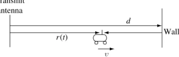
Suppose the receive antenna is now moving at a velocityv(Figure 2.4). As it moves through the pattern of constructive and destructive interference created by the two waves, the strength of the received signal increases and decreases. This is the phenomenon ofmultipath fading. The time taken to travel from a peak to a valley isc/4fv: this is the time-scale at which the fading occurs, and it is called thecoherence timeof the channel.

An equivalent way of seeing this is in terms of the Doppler shifts of the direct and the reflected waves. Suppose the receive antenna is at locationr₀ at time 0. Takingr=r₀+vtin (2.6), we get

E_rf t=cos 2f 1−v/ct−r0/c r₀+vt

−cos 2f 1+v/ct+r0−2d/c

2d−r₀−vt (2.11) The first term, the direct wave, is a sinusoid at frequencyf1−v/c, expe-riencing a Doppler shiftD₁= −fv/c. The second is a sinusoid at frequency f1+v/c, with a Doppler shiftD₂= +fv/c. The parameter

D_s=D₂−D₁ (2.12) is called theDoppler spread. For example, if the mobile is moving at 60 km/h andf =900 MHz, the Doppler spread is 100 Hz. The role of the Doppler spread can be visualized most easily when the mobile is much closer to the wall than to the transmit antenna. In this case the attenuations are roughly the same for both paths, and we can approximate the denominator of the second term byr=r₀+vt. Then, combining the two sinusoids, we get

E_rf t≈2sin 2f vt/c+r0−d/csin 2f t−d/c

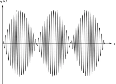
r₀+vt (2.13) This is the product of two sinusoids, one at the input frequencyf, which is typ-ically of the order of GHz, and the other one atfv/c=D_s/2, which might be of the order of 50 Hz. Thus, the response to a sinusoid atf is another sinusoid at f with a time-varying envelope, with peaks going to zeros around every 5 ms (Figure 2.5). The envelope is at its widest when the mobile is at a peak of the

Figure 2.4Illustration of a direct path and a reflected path. Wall Transmit antenna r(t) d υ

(8)

Figure 2.5The received waveform oscillating at frequencyfwith a slowly varying envelope at frequency Ds/2.

t

E_r(t)

interference pattern and at its narrowest when the mobile is at a valley. Thus, the Doppler spread determines the rate of traversal across the interference pattern and is inversely proportional to the coherence time of the channel.

We now see why we have partially ignored the denominator terms in (2.11) and (2.13). When the difference in the length between two paths changes by a quarter wavelength, the phase difference between the responses on the two paths changes by/2, which causes a very significant change in the overall received amplitude. Since the carrier wavelength is very small relative to the path lengths, the time over which this phase effect causes a significant change is far smaller than the time over which the denominator terms cause a significant change. The effect of the phase changes is of the order of milliseconds, whereas the effect of changes in the denominator is of the order of seconds or minutes. In terms of modulation and detection, the time-scales of interest are in the range of milliseconds and less, and the denominators are effectively constant over these periods.

The reader might notice that we are constantly making approximations in trying to understand wireless communication, much more so than for wired communication. This is partly because wired channels are typically time-invariant over a very long time-scale, while wireless channels are typically time-varying, and appropriate models depend very much on the time-scales of interest. For wireless systems, the most important issue is what approximations to make. Thus, it is important to understand these modeling issues thoroughly.

2.1.5 Reflection from a ground plane

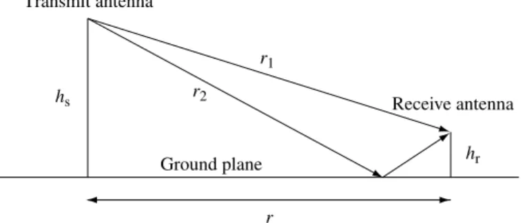
Consider a transmit and a receive antenna, both above a plane surface such as a road (Figure 2.6). When the horizontal distancerbetween the antennas becomes very large relative to their vertical displacements from the ground

(9)

Figure 2.6Illustration of a direct path and a reflected path off a ground plane.

Transmit antenna Ground plane Receive antenna h_r h_s r2 r r₁

plane (i.e., height), a very surprising thing happens. In particular, the differ-ence between the direct path length and the reflected path length goes to zero asr−1_{with increasing}_r_{(Exercise 2.5). When}_r_{is large enough, this difference}

between the path lengths becomes small relative to the wavelengthc/f. Since the sign of the electric field is reversed on the reflected path5_{, these two waves}

start to cancel each other out. The electric wave at the receiver is then attenu-ated asr−2_{, and the received power decreases as}_r−4_{. This situation is}

partic-ularly important in rural areas where base-stations tend to be placed on roads.

2.1.6 Power decay with distance and shadowing

The previous example with reflection from a ground plane suggests that the received power can decrease with distance faster thanr−2_{in the presence of}

disturbances to free space. In practice, there are several obstacles between the transmitter and the receiver and, further, the obstacles might also absorb some power while scattering the rest. Thus, one expects the power decay to be considerably faster thanr−2_{. Indeed, empirical evidence from experimental}

field studies suggests that while power decay near the transmitter is liker−2_,

at large distances the power can even decayexponentiallywith distance. The ray tracing approach used so far provides a high degree of numerical accuracy in determining the electric field at the receiver, but requires a precise physical model including the location of the obstacles. But here, we are only looking for the order of decay of power with distance and can consider an alternative approach. So we look for a model of the physical environment with the fewest parameters but one that still provides useful global information about the field properties. A simple probabilistic model with two parameters of the physical environment, the density of the obstacles and the fraction of energy each object absorbs, is developed in Exercise 2.6. With each obstacle

5 _{This is clearly true if the electric field is parallel to the ground plane. It turns out that this is} also true for arbitrary orientations of the electric field, as long as the ground is not a perfect conductor and the angle of incidence is small enough. The underlying electromagnetics is analyzed in Chapter 2 of Jakes [62].

(10)

absorbing the same fraction of the energy impinging on it, the model allows us to show that the power decays exponentially in distance at a rate that is proportional to the density of the obstacles.

With a limit on the transmit power (either at the base-station or at the mobile), the largest distance between the base-station and a mobile at which communication can reliably take place is called thecoverageof the cell. For reliable communication, a minimal received power level has to be met and thus the fast decay of power with distance constrains cell coverage. On the other hand, rapid signal attenuation with distance is also helpful; it reduces the interferencebetween adjacent cells. As cellular systems become more popular, however, the major determinant of cell size is the number of mobiles in the cell. In engineering jargon, the cell is said to be capacitylimited instead of coverage limited. The size of cells has been steadily decreasing, and one talks of micro cells and pico cells as a response to this effect. With capacity limited cells, the inter-cell interference may be intolerably high. To alleviate the inter-cell interference, neighboring cells use different parts of the frequency spectrum, and frequency is reused at cells that are far enough. Rapid signal attenuation with distance allows frequencies to be reused at closer distances. The density of obstacles between the transmit and receive antennas depends very much on the physical environment. For example, outdoor plains have very little by way of obstacles while indoor environments pose many obsta-cles. This randomness in the environment is captured by modeling the density of obstacles and their absorption behavior as random numbers; the overall phenomenon is calledshadowing.6_{The effect of shadow fading differs from}

multipath fading in an important way. The duration of a shadow fade lasts for multiple seconds or minutes, and hence occurs at a much slower time-scale compared to multipath fading.

2.1.7 Moving antenna, multiple reflectors

Dealing with multiple reflectors, using the technique of ray tracing, is in principle simply a matter of modeling the received waveform as the sum of the responses from the different paths rather than just two paths. We have seen enough exam-ples, however, to understand that finding the magnitudes and phases of these responses is no simple task. Even for the very simple large wall example in Figure 2.2, the reflected field calculated in (2.6) is valid only at distances from the wall that are small relative to the dimensions of the wall. At very large dis-tances, the total power reflected from the wall is proportional to bothd−2_and

to the area of the cross section of the wall. The power reaching the receiver is proportional tod−rt−2_{. Thus, the power attenuation from transmitter to}

receiver (for the large distance case) is proportional todd−rt−2_rather

(11)

than to2d−rt−2_{. This shows that ray tracing must be used with some}

caution. Fortunately, however, linearity still holds in these more complex cases. Another type of reflection is known as scattering and can occur in the atmosphere or in reflections from very rough objects. Here there are a very large number of individual paths, and the received waveform is better modeled as an integral over paths with infinitesimally small differences in their lengths, rather than as a sum.

Knowing how to find the amplitude of the reflected field from each type of reflector is helpful in determining the coverage of a base-station (although ultimately experimentation is necessary). This is an important topic if our objective is trying to determine where to place base-stations. Studying this in more depth, however, would take us afield and too far into electromagnetic theory. In addition, we are primarily interested in questions of modulation, detection, multiple access, and network protocols rather than location of base-stations. Thus, we turn our attention to understanding the nature of the aggregate received waveform, given a representation for each reflected wave. This leads to modeling the input/output behavior of a channel rather than the detailed response on each path.

2.2 Input/output model of the wireless channel

We derive an input/output model in this section. We first show that the mul-tipath effects can be modeled as a linear time-varying system. We then obtain a baseband representation of this model. The continuous-time channel is then sampled to obtain a discrete-time model. Finally we incorporate additive noise.

2.2.1 The wireless channel as a linear time-varying system

In the previous section we focused on the response to the sinusoidal input t=cos 2ft. The received signal can be written as_ia_if tt−_if t, wherea_if t and_if tare respectively the overall attenuation and prop-agation delay at time t from the transmitter to the receiver on path i. The overall attenuation is simply the product of the attenuation factors due to the antenna pattern of the transmitter and the receiver, the nature of the reflector, as well as a factor that is a function of the distance from the transmitting antenna to the reflector and from the reflector to the receive antenna. We have described the channel effect at a particular frequencyf. If we further assume that thea_if tand the _if t do not depend on the frequencyf, then we can use the principle of superposition to generalize the above input/output relation to an arbitrary inputxtwith non-zero bandwidth:

yt=

i

(12)

21 2.2 Input/output model of the wireless channel

In practice the attenuations and the propagation delays are usually slowly varying functions of frequency. These variations follow from the time-varying path lengths and also from frequency-dependent antenna gains. However, we are primarily interested in transmitting over bands that are narrow relative to the carrier frequency, and over such ranges we can omit this frequency dependence. It should however be noted that although theindividual attenua-tions and delays are assumed to be independent of the frequency, theoverall channel response can still vary with frequency due to the fact that different paths have different delays.

For the example of a perfectly reflecting wall in Figure 2.4, then,

a₁t= r₀+vt a2t= 2d−r₀−vt (2.15) ₁t=r0+vt c − ∠₁ 2f 2t= 2d−r₀−vt c − ∠₂ 2f (2.16)

where the first expression is for the direct path and the second for the reflected path. The term ∠_j here is to account for possible phase changes at the transmitter, reflector, and receiver. For the example here, there is a phase reversal at the reflector so we take₁=0 and₂=.

Since the channel (2.14) is linear, it can be described by the response h t at timet to an impulse transmitted at timet−. In terms of h t, the input/output relationship is given by

yt=

−h txt−d (2.17)

Comparing (2.17) and (2.14), we see that the impulse response for the fading multipath channel is

h t=

i

a_it−_it (2.18) This expression is really quite nice. It says that the effect of mobile users, arbitrarily moving reflectors and absorbers, and all of the complexities of solv-ing Maxwell’s equations, finally reduce to an input/output relation between transmit and receive antennas which is simply represented as the impulse response of a linear time-varying channel filter.

The effect of the Doppler shift is not immediately evident in this repre-sentation. From (2.16) for the single reflecting wall example, _it=v_i/c wherev_i is the velocity with which theith path length is increasing. Thus, the Doppler shift on theith path is−f_it.

In the special case when the transmitter, receiver and the environment are all stationary, the attenuationsa_itand propagation delays_itdo not

(13)

depend on timet, and we have the usual linear time-invariant channel with an impulse response

h=

i

a_i−_i (2.19) For the time-varying impulse responseh t, we can define a time-varying frequency response Hf t = −h te −j2f _d₌ i a_ite−j2fit _(2.20)

In the special case when the channel is time-invariant, this reduces to the usual frequency response. One way of interpretingHf tis to think of the system as a slowly varying function oftwith a frequency responseHf t at each fixed timet. Corresponding,h tcan be thought of as the impulse response of the system at a fixed time t. This is a legitimate and useful way of thinking about many multipath fading channels, as the time-scale at which the channel varies is typically much longer than the delay spread (i.e., the amount of memory) of the impulse response at a fixed time. In the reflecting wall example in Section 2.1.4, the time taken for the channel to change significantly is of the order of milliseconds while the delay spread is of the order of microseconds. Fading channels which have this characteristic are sometimes calledunderspreadchannels.

2.2.2 Baseband equivalent model

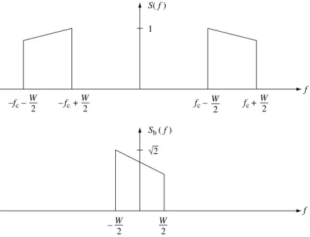
In typical wireless applications, communication occurs in a passband f_c−W/2 f_c+W/2 of bandwidth W around a center frequency f_c, the spectrum having been specified by regulatory authorities. However, most of the processing, such as coding/decoding, modulation/demodulation, synchronization, etc., is actually done at the baseband. At the transmitter, the last stage of the operation is to “up-convert” the signal to the carrier frequency and transmit it via the antenna. Similarly, the first step at the receiver is to “down-convert” the RF (radio-frequency) signal to the baseband before further processing. Therefore from a communication system design point of view, it is most useful to have a baseband equivalent representation of the system. We first start with defining the baseband equivalent representation of signals. Consider a real signal stwith Fourier transform Sf , band-limited in f_c−W/2 f_c+W/2withW <2f_c. Define itscomplex baseband equivalent s_btas the signal having Fourier transform:

S_bf =

√

2Sf+f_c f+f_c>0

(14)

Figure 2.7Illustration of the relationship between a passband spectrumS(f )and its baseband equivalent Sb(f ).

W 2 1 S_b( f ) S( f ) f f –f_c –W 2 fc – W 2 – f_c W 2 + W 2 f_c+ W 2 – 2 √

Sincestis real, its Fourier transform satisfiesSf =S∗−f , which means that s_btcontains exactly the same information asst. The factor of√2 is quite arbitrary but chosen to normalize the energies of s_btand stto be the same. Note thats_btis band-limited in−W/2 W/2. See Figure 2.7.

To reconstructstfroms_bt, we observe that

√

2Sf =S_bf−f_c+S_b∗−f−f_c (2.22) Taking inverse Fourier transforms, we get

st=√1 2 s_btej2fct+_s∗ bte− j2fct=√₂_s bte j2fct _(2.23)

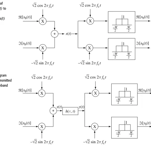
In terms of real signals, the relationship between st and s_bt is shown in Figure 2.8. The passband signal st is obtained by modulating

s_bt by √2 cos 2f_ct and s_bt by −√2 sin 2f_ct and summing, to get√2s_btej2fct_{(up-conversion). The baseband signal}_s

bt

(respec-tively s_bt) is obtained by modulating st by √2 cos 2f_ct (respec-tively −√2 sin 2f_ct) followed by ideal low-pass filtering at the baseband −W/2 W/2(down-conversion).

Let us now go back to the multipath fading channel (2.14) with impulse response given by (2.18). Let x_bt and y_bt be the complex baseband equivalents of the transmitted signal xt and the received signal yt, respectively. Figure 2.9 shows the system diagram from x_bttoy_bt. This implementation of a passband communication system is known asquadrature amplitude modulation (QAM). The signalx_btis sometimes called the

(15)

Figure 2.8Illustration of upconversion from sb(t)to s(t), followed by downconversion froms(t) back to sb(t). X X X X [s_b(t)] [s_b(t)] [s_b(t)] [s_b(t)] –√2 sin 2πf_ct –√2 sin 2πf_ct √2 cos 2πf_ct √2 cos 2πf_ct s(t) –W 2 W 2 –W 2 W 2 1 1 +

Figure 2.9System diagram from the baseband transmitted signal xb(t)to the baseband received signal yb(t). X X X X [x_b(t)] [x_b(t)] [y_b(t)] [y_b(t)] –W 2 W 2 –W 2 W 2 1 1 + x(t) _h₍_τ_,_t₎ y(t) –√2 sin 2πf_ct –√2 sin 2πf_ct √2 cos 2πf_ct √2 cos 2πf_ct

in-phase component I and x_bt the quadrature component Q (rotated by /2). We now calculate the baseband equivalent channel. Substituting xt=√2x_btej2fct_and_yt=√₂_y btej2fctinto (2.14) we get y_btej2fct = i a_itx_bt−_itej2fct−it = i a_itx_bt−_ite−j2fcit ej2fct (2.24)

Similarly, one can obtain (Exercise 2.13)

y_btej2fct= i a_itx_bt−_ite−j2fcit ej2fct (2.25)

Hence, the baseband equivalent channel is

y_bt=

i

(16)

where

ab_it =a_ite−j2fcit _(2.27)

The input/output relationship in (2.26) is also that of a linear time-varying system, and the baseband equivalent impulse response is

h_b t=

i

ab_it−_it (2.28) This representation is easy to interpret in the time domain, where the effect of the carrier frequency can be seen explicitly. The baseband output is the sum, over each path, of the delayed replicas of the baseband input. The magnitude of theith such term is the magnitude of the response on the given path; this changes slowly, with significant changes occurring on the order of seconds or more. The phase is changed by/2 (i.e., is changed significantly) when the delay on the path changes by 1/4f_c, or equivalently, when the path length changes by a quarter wavelength, i.e., by c/4f_c. If the path length is changing at velocity v, the time required for such a phase change is c/4f_cv. Recalling that the Doppler shift D at frequencyf isfv/c, and noting that f ≈f_c for narrowband communication, the time required for a /2 phase change is 1/4D. For the single reflecting wall example, this is about 5 ms (assumingf_c=900 MHz and v=60 km/h). The phases of both paths are rotating at this rate but in opposite directions.

Note that the Fourier transformH_bf tof h_b tfor a fixedtis simply Hf+f_c t, i.e., the frequency response of the original system (at a fixedt) shifted by the carrier frequency. This provides another way of thinking about the baseband equivalent channel.

2.2.3 A discrete-time baseband model

The next step in creating a useful channel model is to convert the continuous-time channel to a discrete-continuous-time channel. We take the usual approach of the sampling theorem. Assume that the input waveform is band-limited to W. The baseband equivalent is then limited toW/2 and can be represented as

x_bt=

n

xnsincWt−n (2.29)

wherexnis given byx_bn/Wand sinctis defined as

sinct =sint

t (2.30)

This representation follows from the sampling theorem, which says that any waveform band-limited to W/2 can be expanded in terms of the orthogonal

(17)

basissincWt−n_n, with coefficients given by the samples (taken uniformly at integer multiples of 1/W).

Using (2.26), the baseband output is given by

y_bt= n xn i ab itsincWt−Wit−n (2.31)

The sampled outputs at multiples of 1/W, ym =y_bm/W , are then given by ym= n xn i ab_im/W sincm−n−_im/W W (2.32) The sampled outputym can equivalently be thought of as the projection of the waveformy_bt onto the waveformWsincWt−m. Let =m−n. Then ym= xm− i ab_im/W sinc−_im/W W (2.33) By defining hm = i ab_im/W sinc−_im/W W (2.34) (2.33) can be written in the simple form

ym=

hm xm− (2.35) We denotehmas theth (complex) channel filter tap at timem. Its value is a function of mainly the gainsab

it of the paths, whose delaysit are

close to/W (Figure 2.10). In the special case where the gainsab

itand the

delays_itof the paths are time-invariant, (2.34) simplifies to

h=

i

ab_i sinc−_iW (2.36) and the channel is linear time-invariant. The th tap can be interpreted as the sample/W th of the low-pass filtered baseband channel responseh_b (cf. (2.19)) convolved with sinc(W).

We can interpret the sampling operation as modulation and demodulation in a communication system. At timen, we are modulating the complex symbol xm (in-phase plus quadrature components) by the sinc pulse before the up-conversion. At the receiver, the received signal is sampled at timesm/W

(18)

Figure 2.10Due to the decay of the sinc function, theith path contributes most significantly to theth tap if its delay falls in the window

/W−1/2W /W+ 1/2W . 1 W Main contribution l = 0 Main contribution l = 0 Main contribution l = 1 Main contribution l = 2 Main contribution l = 2 i=0 i=1 i=2 i=3 i=4 0 1 2 l

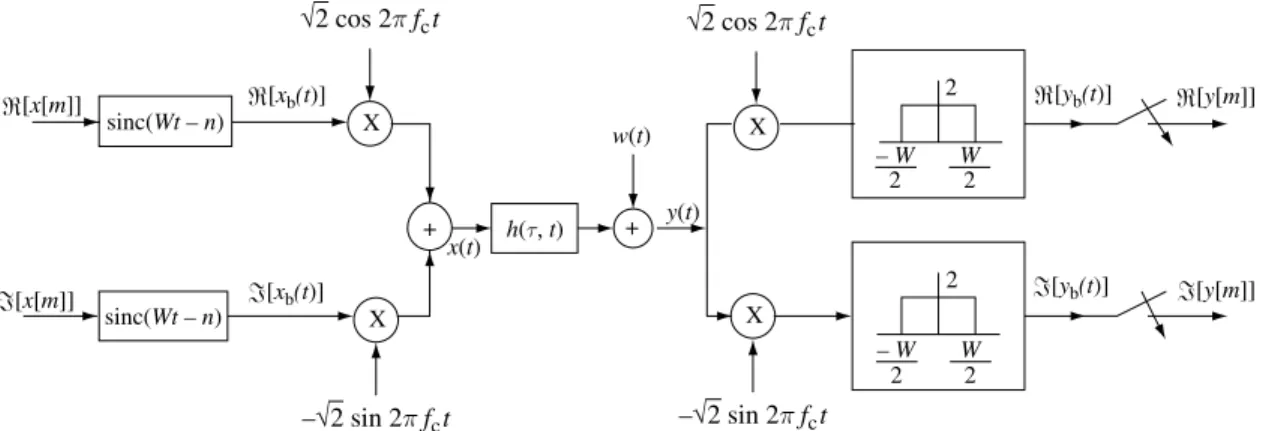
at the output of the low-pass filter. Figure 2.11 shows the complete system. In practice, other transmit pulses, such as the raised cosine pulse, are often used in place of the sinc pulse, which has rather poor time-decay property and tends to be more susceptible to timing errors. This necessitates sampling at the Nyquist sampling rate, but does not alter the essential nature of the model. Hence we will confine to Nyquist sampling.

Due to the Doppler spread, the bandwidth of the outputy_btis generally slightly larger than the bandwidthW/2 of the inputx_bt, and thus the output samplesymdo not fully represent the output waveform. This problem is usually ignored in practice, since the Doppler spread is small (of the order of tens to hundreds of Hz) compared to the bandwidth W. Also, it is very convenient for the sampling rate of the input and output to be the same. Alternatively, it would be possible to sample the output at twice the rate of the input. This would recapture all the information in the received waveform.

(19)

X X X X [x[m]] sinc (Wt – n) [x[m]] sinc (Wt – n) h(τ, t) 1 –W W –W W 1 + [x_b(t)] [y[m]] [y[m]] [y_b(t)] [y_b(t)] y(t) x(t) [x_b(t)] 2 2 2 2 –√2 sin 2πf_ct –√2 sin 2πf_ct √2 cos 2πf_ct √2 cos 2πf_ct

The number of taps would be almost doubled because of the reduced sample Figure 2.11System diagram

from the baseband transmitted symbolx[m] to the baseband sampled received signaly[m].

interval, but it would typically be somewhat less than doubled since the representation would not spread the path delays so much.

Discussion 2.1 Degrees of freedom

The symbol xm is the mth sample of the transmitted signal; there are W samples per second. Each symbol is a complex number; we say that it represents one (complex)dimensionordegree of freedom. The continuous-time signalxtof duration one second corresponds toW discrete symbols; thus we could say that the band-limited, continuous-time signal has W degrees of freedom, per second.

The mathematical justification for this interpretation comes from the following important result in communication theory: the signal space of complex continuous-time signals of duration T which have most of their energy within the frequency band −W/2 W/2 has dimension approx-imately WT. (A precise statement of this result is in standard com-munication theory text/books; see Section 5.3 of [148] for example.) This result reinforces our interpretation that a continuous-time signal with bandwidth W can be represented by W complex dimensions per second.

The received signalytis also band-limited to approximatelyW (due to the Doppler spread, the bandwidth is slightly larger thanW) and hasW complex dimensions per second. From the point of view of communication over the channel, the received signal space is what matters because it dictates the number of different signals which can be reliably distinguished at the receiver. Thus, we define the degrees of freedom of the channel to be the dimension of the received signal space, and whenever we refer to the signal space, we implicitly mean the received signal space unless stated otherwise.

(20)

2.2.4 Additive white noise

As a last step, we include additive noise in our input/output model. We make the standard assumption thatwtis zero-mean additive white Gaussian noise (AWGN) with power spectral densityN₀/2 (i.e.,Ew0wt=N₀/2t. The model (2.14) is now modified to be

yt=

i

a_itxt−_it+wt (2.37) See Figure 2.12. The discrete-time baseband-equivalent model (2.35) now becomes

ym=

hmxm−+wm (2.38) where wm is the low-pass filtered noise at the sampling instant m/W. Just like the signal, the white noise wt is down-converted, filtered at the baseband and ideally sampled. Thus, it can be verified (Exercise 2.11) that

wm = −wtm1tdt (2.39) wm = −wtm2tdt (2.40) where _m₁t = √2Wcos2f_ctsincWt−m _m₂t = −√2Wsin2f_ctsincWt−m (2.41) It can further be shown that_m₁t _m₂t_mforms anorthonormal setof waveforms, i.e., the waveforms are orthogonal to each other (Exercise 2.12). In Appendix A we review the definition and basic properties of white Gaus-sian random vectors (i.e., vectors whose components are independent and identically distributed (i.i.d.) Gaussian random variables). A key property is that the projections of a white Gaussian random vector onto any orthonor-mal vectors are independent and identically distributed Gaussian random variables. Heuristically, one can think of continuous-time Gaussian white noise as an infinite-dimensional white random vector and the above prop-erty carries through: the projections onto orthogonal waveforms are uncorre-lated and hence independent. Hence the discrete-time noise process wm is white, i.e., independent over time; moreover, the real and imaginary components are i.i.d. Gaussians with variances N₀/2. A complex Gaussian random variable X whose real and imaginary components are i.i.d. satis-fies a circular symmetry property: ej_X _{has the same distribution as} _X _for

(21)

X X X X [x[m]] [y[m]] [y[m]] [x[m]] [xb(t)] [yb(t)] [yb(t)] [xb(t)] sinc(Wt – n) sinc(Wt – n) w(t) y(t) x(t) h(τ, t) + + W 2 2 – W 2 W 2 2 – W 2 –√2 sin 2πf_ct –√2 sin 2πf_ct √2 cos 2πf_ct √2 cos 2πf_ct

Gaussian, denoted by 0 2_{, where}2₌_E_X2_{. The concept of}

cir-Figure 2.12A complete system

diagram. _{cular symmetry is discussed further in Section A.1.3 of Appendix A.} The assumption of AWGN essentially means that we are assuming that the primary source of the noise is at the receiver or is radiation impinging on the receiver that is independent of the paths over which the signal is being received. This is normally a very good assumption for most communication situations.

2.3 Time and frequency coherence

2.3.1 Doppler spread and coherence time

An important channel parameter is the time-scale of the variation of the channel. How fast do the tapshmvary as a function of timem? Recall that

hm= i ab im/W sinc−im/W W = i a_im/W e−j2fcim/W _sinc− im/W W (2.42)

Let us look at this expression term by term. From Section 2.2.2 we gather that significant changes ina_i occur over periods of seconds or more. Significant changes in the phase of the ith path occur at intervals of 1/4D_i, where D_i=f_c_it is the Doppler shift for that path. When the different paths contributing to the th tap have different Doppler shifts, the magnitude of hm changes significantly. This is happening at the time-scale inversely proportional to the largest difference between the Doppler shifts, theDoppler spreadD_s:

D_s=max

i j fc

(22)

31 2.3 Time and frequency coherence

where the maximum is taken over all the paths that contribute significantly to a tap.7_{Typical intervals for such changes are on the order of 10 ms. Finally,}

changes in the sinc term of (2.42) due to the time variation of each_itare proportional to the bandwidth, whereas those in the phase are proportional to the carrier frequency, which is typically much larger. Essentially, it takes much longer for a path to move from one tap to the next than for its phase to change significantly. Thus, the fastest changes in the filter taps occur because of the phase changes, and these are significant over delay changes of 1/4D_s.

The coherence time T_c of a wireless channel is defined (in an order of magnitude sense) as the interval over whichhmchanges significantly as a function ofm. What we have found, then, is the important relation

T_c= 1

4D_s (2.44)

This is a somewhat imprecise relation, since the largest Doppler shifts may belong to paths that are too weak to make a difference. We could also view a phase change of/4 to be significant, and thus replace the factor of 4 above by 8. Many people instead replace the factor of 4 by 1. The important thing is to recognize that the major effect in determining time coherence is the Doppler spread, and that the relationship is reciprocal; the larger the Doppler spread, the smaller the time coherence.

In the wireless communication literature, channels are often categorized as fast fadingandslow fading, but there is little consensus on what these terms mean. In this book, we will call a channel fast fading if the coherence timeT_c is much shorter than the delay requirement of the application, and slow fading if T_c is longer. The operational significance of this definition is that, in a fast fading channel, one can transmit the coded symbols over multiple fades of the channel, while in a slow fading channel, one cannot. Thus, whether a channel is fast or slow fading depends not only on the environment but also on the application; voice, for example, typically has a short delay requirement of less than 100 ms, while some types of data applications can have a laxer delay requirement.

2.3.2 Delay spread and coherence bandwidth

Another important general parameter of a wireless system is the multipath delay spread,T_d, defined as the difference in propagation time between the

7 _{The Doppler spread can in principle be different for different taps. Exercise 2.10 explores} this possibility.

(23)

longest and shortest path, counting only the paths with significant energy. Thus,

T_d=max

i j it−jt (2.45)

This is defined as a function oft, but we regard it as an order of magnitude quantity, like the time coherence and Doppler spread. If a cell or LAN has a linear extent of a few kilometers or less, it is very unlikely to have path lengths that differ by more than 300 to 600 meters. This corresponds to path delays of one or two microseconds. As cells become smaller due to increased cellular usage, T_d also shrinks. As was already mentioned, typical wireless channels are underspread, which means that the delay spread T_d is much smaller than the coherence timeT_c.

The bandwidths of cellular systems range between several hundred kilohertz and several megahertz, and thus, for the above multipath delay spread values, all the path delays in (2.34) lie within the peaks of two or three sinc functions; more often, they lie within a single peak. Adding a few extra taps to each channel filter because of the slow decay of the sinc function, we see that cellular channels can be represented with at most four or five channel filter taps. On the other hand, there is a recent interest inultra-wideband(UWB) communication, operating from 3.1 to 10.6 GHz. These channels can have up to a few hundred taps.

When we study modulation and detection for cellular systems, we shall see that the receiver must estimate the values of these channel filter taps. The taps are estimated via transmitted and received waveforms, and thus the receiver makes no explicit use of (and usually does not have) any information about individual path delays and path strengths. This is why we have not studied the details of propagation over multiple paths with complicated types of reflection mechanisms. All we really need is the aggregate values of gross physical mechanisms such as Doppler spread, coherence time, and multipath spread.

The delay spread of the channel dictates itsfrequency coherence. Wireless channels change both in time and frequency. The time coherence shows us how quickly the channel changes in time, and similarly, the frequency coherence shows how quickly it changes in frequency. We first understood about channels changing in time, and correspondingly about the duration of fades, by studying the simple example of a direct path and a single reflected path. That same example also showed us how channels change with frequency. We can see this in terms of the frequency response as well.

Recall that the frequency response at timetis

Hf t=

i

a_ite−j2fit _(2.46)

The contribution due to a particular path has a phase linear inf. For mul-tiple paths, there is a differential phase, 2f_it−_kt. This differential

(24)

33 2.3 Time and frequency coherence 10 0.55 0.6 0.65 0.7 0.75 0.8 0.85 0.9 0.95 1 –60 –50 –40 –30 –20 –10 0 0.65 0.66 0.67 0.68 0.69 0.7 0.71 0.72 0.73 0.74 0.75 0.76 0.45 0 –10 –20 –0.001 –0.0008 –0.0006 –0.0004 –0.0002 0 0.0002 0.0004 0.0006 0.0008 0.001 0 50 100 150 200 250 300 350 400 450 500 550 –30 –40 –50 –60 –70 –0.006 –0.005 –0.004 –0.003 –0.002 –0.001 0 0.001 0.002 0.003 0.004 50 100 150 200 250 300 350 400 450 500 550 0 0.5 (d) Power spectrum (dB) Power specturm (dB)

Amplitude _{(linear scale)} Amplitude _{(linear scale)}

(b) Time (ns) Time (ns) (a) (c) 40 MHz Frequency (GHz) Frequency (GHz) 200 MHz

phase causes selective fading in frequency. This says that E_rf t changes Figure 2.13(a) A channel over

200MHz is frequency-selective, and the impulse response has many taps. (b) The spectral content of the same channel. (c) The same channel over 40MHz is flatter, and has for fewer taps. (d) The spectral contents of the same channel, limited to 40MHz bandwidth. At larger bandwidths, the same physical paths are resolved into a finer resolution.

significantly, not only whentchanges by 1/4D_s, but also whenf changes by 1/2T_d. This argument extends to an arbitrary number of paths, so the coherence bandwidth,W_c, is given by

W_c= 1

2T_d (2.47)

This relationship, like (2.44), is intended as an order of magnitude relation, essentially pointing out that the coherence bandwidth is reciprocal to the multipath spread. When the bandwidth of the input is considerably less than W_c, the channel is usually referred to asflat fading. In this case, the delay spread T_d is much less than the symbol time 1/W, and a single channel filter tap is sufficient to represent the channel. When the bandwidth is much larger than W_c, the channel is said to be frequency-selective, and it has to be represented by multiple taps. Note that flat or frequency-selective fading is not a property of the channel alone, but of the relationship between the bandwidthW and the coherence bandwidthT_d (Figure 2.13).

The physical parameters and the time-scale of change of key parameters of the discrete-time baseband channel model are summarized in Table 2.1. The different types of channels are summarized in Table 2.2.

(25)

Table 2.1A summary of the physical parameters of the channel and the time-scale of change of the key parameters in its discrete-time baseband model.

Key channel parameters and time-scales Symbol Representative values

Carrier frequency f_c 1 GHz

Communication bandwidth W 1 MHz

Distance between transmitter and receiver d 1 km

Velocity of mobile v 64 km/h

Doppler shift for a path D=fcv/c 50 Hz Doppler spread of paths corresponding to

a tap Ds 100 Hz

Time-scale for change of path amplitude d/v 1 minute Time-scale for change of path phase 1/4D 5 ms Time-scale for a path to move over a tap c/vW 20 s

Coherence time Tc=1/4Ds 2.5 ms

Delay spread Td 1s

Coherence bandwidth Wc=1/2Td 500 kHz

Table 2.2A summary of the types of wireless channels and their defining characteristics. Types of channel Defining characteristic Fast fading Tcdelay requirement Slow fading Tcdelay requirement

Flat fading WWc

Frequency-selective fading WWc

Underspread TdTc

2.4 Statistical channel models

2.4.1 Modeling philosophy

We defined Doppler spread and multipath spread in the previous section as quantities associated with a given receiver at a given location, velocity, and time. However, we are interested in a characterization that is valid over some range of conditions. That is, we recognize that the channel filter taps {hm} must be measured, but we want a statistical characterization of how many taps are necessary, how quickly they change and how much they vary.

Such a characterization requires a probabilistic model of the channel tap values, perhaps gathered by statistical measurements of the channel. We are familiar with describing additive noise by such a probabilistic model (as a Gaussian random variable). We are also familiar with evaluating error probability while communicating over a channel using such models. These

(26)

35 2.4 Statistical channel models

error probability evaluations, however, depend critically on the independence and Gaussian distribution of the noise variables.

It should be clear from the description of the physical mechanisms gener-ating Doppler spread and multipath spread that probabilistic models for the channel filter taps are going to be far less believable than the models for additive noise. On the other hand, we need such models, even if they are quite inaccurate. Without models, systems are designed using experience and experimentation, and creativity becomes somewhat stifled. Even with highly over-simplified models, we can compare different system approaches and get a sense of what types of approaches are worth pursuing.

To a certain extent, all analytical work is done with simplified models. For example, white Gaussian noise (WGN) is often assumed in communication models, although we know the model is valid only over sufficiently small frequency bands. With WGN, however, we expect the model to be quite good when used properly. For wireless channel models, however, probabilistic models are quite poor and only provide order-of-magnitude guides to system design and performance. We will see that we can define Doppler spread, multi-path spread, etc. much more cleanly with probabilistic models, but the underly-ing problem remains that these channels are very different from each other and cannot really be characterized by probabilistic models. At the same time, there is a large literature based on probabilistic models for wireless channels, and it has been highly useful for providing insight into wireless systems. However, it is important to understand the robustness of results based on these models. There is another question in deciding what to model. Recall the continuous-time multipath fading channel

yt=

i

a_itxt−_it+wt (2.48) This contains an exact specification of the delay and magnitude of each path. From this, we derived a discrete-time baseband model in terms of channel filter taps as ym= hmxm−+wm (2.49) where hm= i a_im/W e−j2fcim/W _sinc− im/W W (2.50)

We used the sampling theorem expansion in which xm=x_bm/W and ym=y_bm/W . Each channel tap hm contains an aggregate of paths, with the delays smoothed out by the baseband signal bandwidth.

Fortunately, it is the filter taps that must be modeled for input/output descriptions, and also fortunately, the filter taps often contain a sufficient path aggregation so that a statistical model might have a chance of success.

(27)

2.4.2 Rayleigh and Rician fading

The simplest probabilistic model for the channel filter taps is based on the assumption that there are a large number of statistically independent reflected and scattered paths with random amplitudes in the delay window cor-responding to a single tap. The phase of theith path is 2f_c_imodulo 2. Now, f_c_i=d_i/, whered_iis the distance travelled by theith path andis the carrier wavelength. Since the reflectors and scatterers are far away relative to the car-rier wavelength, i.e.,d_i, it is reasonable to assume that the phase for each path is uniformly distributed between 0 and 2and that the phases of different paths are independent. The contribution of each path in the tap gainhmis

a_im/W e−j2fcim/W _sinc−

im/W W (2.51)

and this can be modeled as a circular symmetric complex random variable.8

Each tap hm is the sum of a large number of such small independent circular symmetric random variables. It follows thathmis the sum of many small independent real random variables, and so by the Central Limit Theorem, it can reasonably be modeled as a zero-mean Gaussian random variable. Similarly, because of the uniform phase,hmej _{is Gaussian}

with the same variance for any fixed . This assures us that hm is in fact circular symmetric0 2

(see Section A.1.3 in Appendix A for an

elaboration). It is assumed here that the variance ofhmis a function of the tap, but independent of timem(there is little point in creating a probabilistic model that depends on time). With this assumed Gaussian probability density, we know that the magnitude hm of the th tap is a Rayleigh random variable with density (cf. (A.20) in Appendix A and Exercise 2.14)

x 2 exp −x2 22 x≥0 (2.52) and the squared magnitudehm2_{is exponentially distributed with density}

1 2 exp −x 2 x≥0 (2.53) This model, which is calledRayleigh fading, is quite reasonable for scat-tering mechanisms where there are many small reflectors, but is adopted primarily for its simplicity in typical cellular situations with a relatively small number of reflectors. The wordRayleigh is almost universally used for this

8 _{See Section A.1.3 in Appendix A for a more in-depth discussion of circular symmetric} random variables and vectors.

(28)

model, but the assumption is that the tap gains are circularly symmetric complex Gaussian random variables.

There is a frequently used alternative model in which the line-of-sight path (often called a specularpath) is large and has a known magnitude, and that there are also a large number of independent paths. In this case, hm, at least for one value of, can be modeled as

hm= +1e j₊ 1 +1 0 2 (2.54)

with the first term corresponding to the specular path arriving with uniform phase and the second term corresponding to the aggregation of the large number of reflected and scattered paths, independent of . The parameter (so-called K-factor) is the ratio of the energy in the specular path to the energy in the scattered paths; the larger is, the more deterministic is the channel. The magnitude of such a random variable is said to have aRician distribution. Its density has quite a complicated form; it is often a better model of fading than the Rayleigh model.

2.4.3 Tap gain auto-correlation function

Modeling eachhmas a complex random variable provides part of the statis-tical description that we need, but this is not the most important part. The more important issue is how these quantities vary with time. As we will see in the rest of the book, the rate of channel variation has significant impact on several aspects of the communication problem. A statistical quantity that models this relation-ship is known as thetap gain auto-correlation function,Rn. It is defined as

Rn =h∗mhm+n (2.55) For each tap , this gives the auto-correlation function of the sequence of random variables modeling that tap as it evolves in time. We are tacitly assuming that this is not a function of timem. Since the sequence of random variableshm for any givenhas both a mean and covariance function that does not depend on m, this sequence is wide-sense stationary. We also assume that, as a random variable, hm is independent of hm for all =and allm m. This final assumption is intuitively plausible since paths in different ranges of delay contribute tohmfor different values of.9

The coefficient R0 is proportional to the energy received in the th tap. The multipath spread T_d can be defined as the product of 1/W times the range of which contains most of the total energy ₌₀R0. This is 9 _{One could argue that a moving reflector would gradually travel from the range of one tap to}

(29)

somewhat preferable to our previous “definition” in that the statistical nature ofT_dbecomes explicit and the reliance on some sort of stationarity becomes explicit. Now, we can also define the coherence timeT_c more explicitly as the smallest value of n >0 for which Rn is significantly different from R0. With both of these definitions, we still have the ambiguity of what “significant” means, but we are now facing the reality that these quantities must be viewed as statistics rather than as instantaneous values.

The tap gain auto-correlation function is useful as a way of expressing the statistics for how tap gains change given a particular bandwidthW, but gives little insight into questions related to choice of a bandwidth for communication. If we visualize increasing the bandwidth, we can see several things happening. First, the ranges of delay that are separated into different tapsbecome narrower (1/Wseconds), so there are fewer paths corresponding to each tap, and thus the Rayleigh approximation becomes poorer. Second, the sinc functions of (2.50) become narrower, andR0gives a finer grained picture of the amount of power being received in theth delay window of width 1/W. In summary, as we try to apply this model to largerW, we get more detailed information about delay and correlation at that delay, but the information becomes more questionable.

Example 2.2 Clarke’s model

This is a popular statistical model for flat fading. The transmitter is fixed, the mobile receiver is moving at speed v, and the transmitted signal is scattered by stationary objects around the mobile. There areK paths, the ith path arriving at an angle_i=2i/K,i=0 K−1, with respect to the direction of motion. K is assumed to be large. The scattered path arriving at the mobile at the angle has a delay of t and a time-invariant gaina, and the input/output relationship is given by

yt=

K−1 i=0

a

ixt−it (2.56)

The most general version of the model allows the received power distri-butionpand the antenna gain patternto be arbitrary functions of the angle, but the most common scenario assumes uniform power distri-bution and isotropic antenna gain pattern, i.e., the amplitudesa=a/√K for all angles. This models the situation when the scatterers are located in a ring around the mobile (Figure 2.14). We scale the amplitude of each path by√Kso that the total received energy along all paths isa2_{; for large}

K, the received energy along each path is a small fraction of the total energy. Suppose the communication bandwidth W is much smaller than the reciprocal of the delay spread. The complex baseband channel can be represented by a single tap at each time:

(30)

Rx

Figure 2.14The one-ring model.

The phase of the signal arriving at time 0 from an angle is 2f_c0 mod 2, wheref_c is the carrier frequency. Making the assumption that this phase is uniformly distributed in02and independently distributed across all angles, the tap gain processh₀mis a sum of many small independent contributions, one from each angle. By the Central Limit Theorem, it is reasonable to model the process as Gaussian. Exercise 2.17 shows further that the process is in fact stationary with an autocorrelation functionR₀ngiven by:

R₀n=2a2_J

0nDs/W (2.58)

whereJ₀·is the zeroth-order Bessel function of the first kind: J₀x = 1

0

ejxcosd (2.59)

andD_s=2f_cv/cis the Doppler spread. The power spectral densitySf, defined on−1/2+1/2, is given by Sf= ₄_a2_W Ds √ 1−2fW/Ds2 −D_s/2Wf +D_s/2W 0 else (2.60)

This can be verified by computing the inverse Fourier transform of (2.60) to be (2.58). Plots of the autocorrelation function and the spectrum for are shown in Figure 2.15. If we define the coherence timeT_c to be the value ofn/W such thatR₀n=0 05R₀0, then

T_c=J −1

0 0 05

D_s (2.61)

(31)

2000 2.5 3 3.5 1.5 1 0.5 0 –0.5 –1 –1.5 200 400 600 800 1000 1200 1400 1600 1800 2 R₀[n] –1/2 1/2 S ( f ) –Ds/(2W) 0 Ds/(2W)

Figure 2.15Plots of the auto-correlation function and Doppler spectrum in Clarke’s model.

In Exercise 2.17, you will also verify that Sfdf has the physical interpretation of the received power along paths that have Doppler shifts in the rangef f+df. Thus,Sfis also called theDoppler spectrum. Note thatSfis zero beyond the maximum Doppler shift.

Chapter 2 The main plot

Large-scale fading

Variation of signal strength over distances of the order of cell sizes. Received power decreases with distancer like:

1

r2 (free space)

1

r4 (reflection from ground plane)

(32)

Small-scale fading

Variation of signal strength over distances of the order of the carrier wavelength, due to constructive and destructive interference of multipaths. Key parameters:

Doppler spreadD_s←→coherence timeT_c∼1/D_s

Doppler spread is proportional to the velocity of the mobile and to the angular spread of the arriving paths.

delay spreadT_d←→coherence bandwidthW_c∼1/T_d

Delay spread is proportional to the difference between the lengths of the shortest and the longest paths.

Input/output channel models

• Continuous-time passband (2.14):

yt=

i

a_itxt−_it

• Continuous-time complex baseband (2.26): y_bt=

i

a_ite−j2fcit_x