An Adaptive System for Mode Detection:
How to Deal with Long-Distance Train Trips
Oliver Schweizer
Intitute for Transport Planning and Systems
Swiss Federal Institute of Technology, ETH
Z¨urich, Switzerland
[email protected]
Abstract—This thesis applies a new procedure to accurately detect train trips from GPS-traces. It uses the pre-elaboration (cleaning, trip detection and trip segmentation) introduced in [1] and implements a new train detection method. The new method uses the railway track network to detect train stages. Within such a stage, possible vehicles are searched and the correct one is then selected. The approach was tested on self-collected data. It achieves an accuracy of over 72.8% for long-distance train trips. It improves the accuracy of detection by 53.3% compared to the old algorithm.
I. INTRODUCTION
U
NDERSTANDING and predicting transport behaviour has been a goal of transport engineers for decades. Predicting where the costly investment in the infrastructure leads to the most significant benefit is one of the reasons behind it. In recent years, global problems such as climate change and air pollution became more prominent. Thus, the transport sector is trying to move into a direction where it does not rely on non-renewable energy anymore.Traditionally, travel diaries were the primary source of information for travel behaviour [2]. With the advancement of mobile and information technology, other possibilities to collect data were introduced. These new data sources include, amongst other things, GPS tracking. The cost of the new methods is relatively cheap and not labour intensive compared to travel diaries [3].
Today, GPS-tracking is mainly done by smartphones. How-ever, continuous tracking of the location through GPS places a heavy strain on the battery of mobile phones. For this reason, new systems with low battery consumption were developed. An example of such a system using passive GPS tracking (for long term travel behaviour tracking) is shown in [1]. The algorithm specially developed for this application can detect activities, trips, and transport modes.
This thesis improves the long-distance train detection ca-pabilities of the algorithm introduced in [1]. Firstly, the existing algorithm was studied with a self-collected dataset. By identifying the opportunities and challenges of the existing method, a new sequence specializing in train detection was added.
II. LITERATUREREVIEW
For mode detection, there are four different data sources. The first source is GPS log data, a source that is easily available as with the uprise in smartphones, everyone owns a device capable of logging GPS data. The second one, is the passive tracking data from mobile phone data. The position of mobile phones is tracked every time a call is made or a connection to a new towers is established. The third source is smart card data for automatic fare collection, and the last group is formed by geotagged social media posts. Each of these sources has its own advantages and disadvantages [4].
An analyses on which spatial accuracy and sampling in-tervals perform best is given in [5]. The initial sampling frequency is 1 Hz. Step by step, the sampling intervals are increased to identify which frequency performs best when applying it to several mode detection schemes. The sampling frequency that works best lies within an interval of 30 s to one minute.The same process was repeated for the spacial accuracy, is less critical compared to the sampling frequency. Geographic Information System (GIS) can increase the accuracy of a mode detection algorithm by including transport network information. With the live position of buses, bus stop location and rail line network an accuracy of over 93.5% can be achieved. It improves the accuracy by 17% compared to the approach only using GPS [6].
What makes tracking train trips so tricky? A train carriage is, when simplified, a metal box. For better insulation, the windows of modern trains are coated with a thin metallic film. Inside the train, the radio waves are attenuated as in a Faraday cage [7], leading to a poor performance of GPS tracking inside of trains. For mobile phones, several repeaters inside the carriage help by transmitting the electromagnetic waves used for telecommunications from outside [8].
Overall, many different papers present different approaches of mode detection. Unfortunately, only very few fall into the restricted boundary condition of this thesis, which are given by [1] and the research question.
III. METHODOLOGY
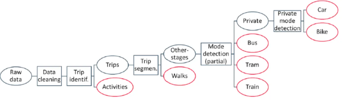
For elaboration of the GPS data in this thesis, a pre-viously developed tool was provided [1]. Figure 1 shows the
in [1].
A. Train Detection
To improve the detection of long-distance train trips, an extensive analysis of the existing algorithm was carried out. By studying the shortcomings of the current solution, valuable information was gathered to find possible approaches for a new solution. A summary of the results of this analysis is found in Chapter IV-B. Before implementing a new method, the existing parameters were modified. The goal was to find better values, especially for train trips. However, the downside of using values streamlined for train travel is a decreased accuracy for all other trip types.
After completing the analysis of the existing model, a new method for train trips was added. As shown in [6], additional geographic information can significantly increase the accuracy of a mode detection. Therefore, the goal is to import not just the position of the stops but also the location of the rails or lines. A method which calculates the rail closeness helps with the identification of all stages travelled by train. The search for train stations is not limited to only the first and last point of a given stage, therefore increasing the chance of finding the right vehicle even with falsely split up stages.
1) Train Network: The network of all rail tracks in Switzer-land is extracted from Open Street Map [9] on a daily basis. However, as there is not much addition to the existing network, even less so within the time frame of this thesis, the same dump is used for the entire thesis. In Open Street Map (OSM) the tag ”railway” contains all information related to railways. It includes any type of railway including mainlines, metros, monorails and sometimes even model railways. Additionally, it also includes any railway infrastructure (stations, platforms etc.). During the import, the data is cleaned up and only the necessary geographic information is kept.
2) Train Stage: For the detection of journeys, a new stage is added to the existing two. With the newly gathered positioning of the rail network, stages travelled by train can be identified. A new function calculates the Euclidean distance of each point to the closest rail. Several methods were then considered to determine if a stage is labelled as a train-stage.
The simplest method used is the average distance to rails over the stage. If the average is below a set train distance threshold, it is considered a train-stage. The second method uses quartiles (percentage) over the stage instead of the aver-age. Several quartiles were tested to find the optimal solution. The results of the analysis are shown in Section IV-C. Due to the bad performance of stages with minimal points, the train
Starting with the first station, each station gets paired with each following one. As in the existing algorithm, the actual data is used to find any railway vehicles in a time window around the time point. The intersection of the two lists forms all the possible connections in between the two points. This process is repeated for each train station up until the second last railway station.
At this point, the right vehicle must be selected based on a list of possible trips. The first assumption for the selection process is that, if there is a direct connection from the first to the last station, it is seen as the correct one. When several vehicles are found, a likelihood function is used to asses the options. Where no direct connection exists, indirect ones with transfers are considered. For a change of train to be possible, another train must stop at the same place. Therefore, any trains in the list starting at a station where no other train stops are ignored. From the starting point of the stage, the train with the longest possible duration is selected. If several are found, the likelihood function is considered once more for the decision. At the end of the first trip, the process is repeated until the destination of a vehicle is the same as the last train station on the list. If no such connection from the beginning to the end is possible, the longest overall trip within the stage is selected.
B. Z¨urich Main Station
Z¨urich Main Station provided an additional challenge, as it has a total of eight platforms underground. Many long-distance trains depart from the lowest section on platforms 31 to 34. This decreased the accuracy of the GPS-points further. Therefore, a particular case for Z¨urich HB was implemented. The time match threshold for vehicles between Z¨urich Main Station and any other station further away than 20 km is increased. The supplementary time is up to 150 s and increases linearly between 20 km and 90 km. Trips longer than 90 km from Z¨urich HB now have a time match threshold of 450 s.
C. Train Station Stop Points
The dataset used for the position of all public transport (PT) stop points is called Location documentation PT-Swiss (DiDok). It includes a single GPS location for each stop. The positioning of the point for train stations is usually at the ticket counter. For the points, any PT stop within 250 m is considered. When arriving at a train station, the official DiDok-point can be further away than 250 m, especially considering the longest trains are 400 m long.
Fig. 1. Sequence of algorithms used for mode detection. Rectangles indicate algorithms; ovals indicate data; red ovals represent the output. [1]
After checking the position of several stops, some were updated with an additional point to better represent the po-sitioning of the platforms instead of the ticket counter. The two stops concerned were Z¨urich Main Station and Bern.
IV. RESULTS
In this section, the different results are presented. First, some details about the data used for the mode detection is shown. It consists of the data collected by the users and the actual public transport operation data. Then the results of the tuning of the input parameters for the old model. They are followed by the same process for the proposed solutions. In the end, the accuracy of the new model with included rail network is compared to the old algorithm.
A. Data
In total, five different users offered their help to collect data. Next to tracking their activities via the phone application, each user wrote down all journeys in a travel diary for validation purposes. Overall, the dataset consists of 170 days. Four train journeys leading outside of Switzerland were ignored.
Unfortunately, due to the Covid-19 pandemic, travel be-haviour changed dramatically. During the lockdown, many days were spent at home. Therefore, for the second part of the data collection from the middle of March onwards, very few journeys with public transport were made. The data set was split up in two different sets. The first half was used as a training set and the second one for validation purposes.
Table I shows the number of journeys made for each dataset by mode. Although both datasets feature a similar amount of days, the consequences of the lockdown can be seen. However, not all differences are due to the lockdown. Part of the reduction is also a result of tracking of different users with other travel behaviour. Additionally, a substantial decrease in journeys on buses and trams is also due to the seasonal change. In good weather, many of those five users use a bicycle as their primary mode of transport.
1) Data Quality: A comparison of point size before and after the cleaning process by mode measures how accurate the tracking of each mode is. For train journeys, on average 65% of all points get removed. Whereas for bus and tram rides, only 15% are eliminated. It clearly shows the difficulty of tracking a user on a train.
TABLE I
NUMBER OFTRIPS PERMODE
Train Bus/
Tram total long short training 62 41 21 174 validation 23 21 2 17
B. Tuning of the different input parameters
Different input parameters were tested on a ten-day data sample including train journeys. The goal was to find better parameters, which are specially tuned for identifying and splitting up trips that include a stage on a train.
1) Cleaning: Before starting with the identification and segmentation of the trips, the data is cleaned. Within the clean-ing process, one parameter has an impact on train journeys during the filtering of the data. It is the maximum allowed speed. The speed of Intercity trains, on the high-speed tracks, is significantly larger than the maximum achievable speed on rails or highway inside cities. Therefore, the default value of 150 km/h used in [1] is too low. To account for the higher speed, an alternative maximum allowed speed of 220 km/h was tested. This is 10% higher than the maximum speed of trains within Switzerland while running under ETCS Level 2 supervision [10].
Looking at an example train journey from Bern to Z¨urich HB. For the slower allowed speed, a total of 60 valid points remain of the 164 measured points during this stage. The higher allowed speed left 78 data points.
2) Trip Segmentation: Analysing the results showed that for trips with good data points, the trips were split up at each longer stop. In between was a walk-stage for the dwelling time at the train station.
At this point, it was not yet clear if such a walk-stage included a transfer between two different trains or is just a stop. Transfer times of three minutes are not unusual for mid-sized train stations. Therefore, joining too many stages together might lead to a loss of valuable information.
The values of the minimum time for a walk, the time under which small groups between large ones are merged and the time to consider near points to adjust their label were tweaked. No real improvement to the default values was achieved. Therefore, the same parameters as presented in [1] are used
Fig. 2. Accuracy of different rail closeness methods expressed as percentage of correct detected rail stages
for this thesis. The main reason behind the sometimes wrong segmentation is the bad quality of the raw data.
C. Tuning of Rail Closeness Metric
For the rail closeness of a stage, five different metrics are tested on the same ten days as above. The accuracy of each approach is measured by the percentage of correctly identified train stages. For all of them, the distance threshold to be considered a train-stage is 200 m. Figure 2 presents the accuracy of the tuning. There is no difference between the average, median and 60% quartile. The accuracy decreases with higher quartiles, first slightly for the 70% quartile but then drastically for the 80% quartile.
In the given test data set, an additional disadvantage of the current process to detect train stages was found. For stages with few points, even a small number of wrongly placed points have a significant impact on the rail closeness. Therefore, for stages with eight points or less, the distance threshold was increased to 400 m. This results in a further increase of accuracy by two per cent to almost 98% (60% quartile plus). In the following sections, the ‘60% quartile plus’ method is used to calculate the rail closeness over a stage.
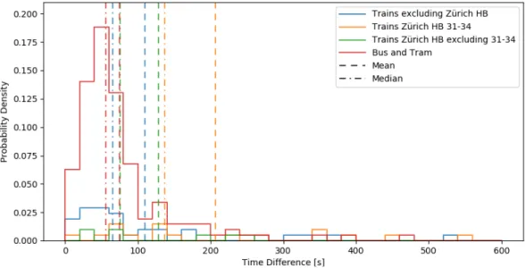
D. Time Difference
While studying the shortcomings of the previous algorithm, a difficulty in the correct detection at Z¨urich Main Station was noticed. Figure 3 shows the distribution of the time difference for the different modes. The train trips are split up into three different sections. One section includes all trips except those arriving or departing at Z¨urich Main Station. The other sections include stages from Z¨urich Main Station which are split up into two groups, one leaving from platform 31 to 34 and the other for all other platforms. Not included in the Z¨urich Main Station set are the trains leaving from Z¨urich HB SZU (platform 21 and 22) as it is classified as a separate train station.
The time difference for Bahnhof L¨owenstrasse (platform 31-34) is significantly larger than any other. In contrast, all other platforms in Z¨urich Main Station only have a slightly
101 s and a median value of 65 s. Without including Bahnhof L¨owenstrasse the two results are almost identical.
E. Accuracy of the Mode Detection Algorithm
Table II shows the results of the mode detection for the algorithm presented in [1] and with the proposed solution. The accuracy of train trips is higher by 45.2% and 43.5% for the training and validation set respectively. Only looking at long-distance train rides the increase is even more significant with 53.6% and 52.4%.
The accuracy of the tram and bus rides remains unchanged. Over all days, only one less trip for each mode was detected with the new algorithm. However, there are now some false positive train trips detected. In each dataset, three incorrect train vehicles are present.
V. DISCUSSION
The dataset for the testing includes many different long-distance train trips. Almost every major train station within Switzerland is represented at least once. Unfortunately, due to the circumstances, the validation set is smaller. Luckily the decrease in train trips is not as significant than the one for tram and bus rides. Due to the few journeys in the second dataset, proper validation of the new process is only limitedly possible.
The parameters of the old models remained unchanged. The results from [1] and the ones presented here are therefore comparable, as the same process is used just on a different dataset. The reason for keeping the same parameters for the trip segmentation and identification is that no better solution was found. It also made the process easier as the first part of the algorithm could remain unchanged.
The only room for improvement is by increasing the max-imum allowed speed. A speed of only 150 km/h filters too many points on the high-speed rail lines. Therefore, changing the value to 220 km/h would have been the better option. Unfortunately, the discovery of this fact occurred after all data sets were already identified.
The higher allowed speed would not have increased the mode detection accuracy of the proposed solution. Currently the way the solution is implemented, it does not matter how many points are between two stops. The old model, on the other hand, would profit from the additional points along the railway line. The splitting up of train journeys into too many small stages could mean that the algorithm is not able not find the right vehicle. Currently, only two adjacent non-matched stages are merged into a single stage for a second try at
Fig. 3. Distribution of the time difference for the detected stages (grouped each 20 s) TABLE II
MODE DETECTION ACCURACY FOR EACH DATASET,EXPRESSED AS PERCENTAGE OF CORRECT DETECTION
[1] proposed solution
Train Bus/
Tram
Train Bus/
Tram [%] total long short total long short
training correct 32.26 21.95 52.38 56.9 77.42 75.61 80.95 56.32 partly correct 14.52 14.63 14.29 16.09 6.45 7.32 4.76 16.09 not found 53.23 65.85 28.57 27.01 16.13 17.07 14.29 27.59 false positive 0.0 0.0 0.0 - 4.84 4.88 4.76 -v alidation correct 21.74 14.29 0.0 58.82 65.22 66.67 50.50 58.82 partly correct 34.78 38.1 0.0 29.41 26.09 23.81 50.50 29.41 not found 52.17 47.62 10.00 11.76 4.35 4.76 0.0 11.76 false positive 0.0 0.0 0.0 - 13.04 14.29 0.0
-matching. Train trips divided into three or more other-stages will therefore remain undetected.
Tuning the new metric for the detection of train stages resulted in equally accurate solutions. Comparing the accuracy of the chosen subset of the testing data, no difference was seen between the first three options (average, median and 60% quartile). Therefore, none of them is clearly a better choice. In the end, the 60% quartile plus was used for all subsequent tests and validation. However, using an average metric adapted with the plus would have most likely resulted in the same outcomes. The additional points added to the service point-data for Z¨urich Main Station and Bern make a considerable difference for the detection of the arrival and departure at both these stations. For both train stations, the official point only covers roughly 50% of the platform area. With the new points, all platforms are covered by the detection radius of 250 m.
Z¨urich Main Station itself remains a challenge, especially Bahnhof L¨owenstrasse. Adding together the bad reception inside the wagon and the tunnel of the train station, the data quality decreases drastically. In the most extreme cases, the GPS points are up to 900 m away from the actual position of the user, while sitting in a train waiting for departure.
By increasing the time match threshold, especially for
long-distance trips, the poor quality of the data can be counteracted. Figure 3 clearly shows the distinction between the time difference. Generally, the impact is seen on all train trips. Nevertheless, not to the same extent as trips which depart from Bahnhof L¨owenstrasse in Z¨urich. As the increase is tied to the distance to Z¨urich Main station, false positives on short S-Bahn trips can be avoided. The added time threshold of 150 s is set to include the longest dwelling time of an intercity train at the station.
Including the rail network as an additional method to detect train stages leads to a significant increase in train detection accuracy. In total, 77.4% are identified correctly for the training dataset and 65.2% for the validation dataset. In addition to the entirely correct identified train journeys, there are another 6.4% and 26% partly identified trips. Here most of the time, the last or first stop are not recognised. Overall, only 16.1% during the training and 4.3% during the validation phases remain unidentified. Comparing the results to the one achieved in [1], it is an increase in train detection accuracy form 68.8% to 78.2%, but now including long-distance trips. This has been done without affecting the accuracy of the other modes.
proposed algorithm can overwrite already matched stages is that testing was only done with operational data of train trips. The performance for searching through a couple ten thousand train trips rather than hundreds of thousands of PT trips was a lot better and thus used for implementing and testing the new method.
Adding together the partly detected and fully detected train trips gives a better performance for the validation dataset. One reason being the slightly better quality of the data for the second part. Also, there were fewer trips involving Z¨urich HB, which made the detection slightly easier. The proposed solution performs better on long-distance trips than short-distance ones. A possible explanation of this is the longer transfer times at larger stations. Therefore, more time is available for a GPS point within the radius of the train station. Something that has not yet been talked about, is the time it takes to compute the mode detection. Calculating the train closeness takes under a second for each day, which is barely noticeable. Searching for the close-by train station is also done quickly as the PT stop file can be filtered for only train stations. It leaves only 1700 points to compare to, which also takes less than a second for each train-stage. However, where the time drastically increases, is searching for vehicles within the time distance threshold at each stop. There is no shortened train vehicle list, and thus the search goes through millions of vehicle stops in Switzerland. Depending on the number of stations along a train stage, looking for vehicles can take up to ten times as long as the previous algorithm did.
VI. CONCLUSION ANDOUTLOOK
The new approach significantly increased the accuracy of the long-distance train trips, while still keeping the accuracy for all other modes the same. It shows that by using additional GIS information of the rail network, the detection of train stages can be improved. Thus making it easier to detect the origin and destination of a train journey.
The proposed solution was only tested on a small self-collected dataset. Nevertheless, the five users taking part in the study managed to travel to almost all larger train stations in Switzerland. The most significant amount of data was collected on the intercity between Z¨urich and Bern. This is inconvenient, as Z¨urich Main Station proved to be the biggest challenge for the mode detection.
The biggest downside is the long computation time. This is because a significant increase in searches through the actual data is necessary to match the exact vehicle. By pre-sorting the train stations, the process could be sped up. Any railway
to reach an accuracy of over 90% with this approach. Not finding the correct destination, origin or a too significant time difference makes the matching with the operational data impossible. Currently, a new type of train window is being research. The goal is to combine mobile reception and thermal insulation [11]. Radio waves from GPS satellites operate in the same range as mobile telephone signals; these would then be able to pass through the windows as well. Thus, the tracking quality of users on board trains would increase.
REFERENCES
[1] A. D. Marra, H. Becker, K. W. Axhausen, and F. Corman, “Developing a passive gps tracking system to study long-term travel behavior,”
Transportation Research Part C: Emerging Technologies, vol. 104, pp. 348 – 368, 2019. [Online]. Available: http://www.sciencedirect.com/ science/article/pii/S0968090X18315729
[2] R. Schlich and K. W. Axhausen, “Habitual travel behaviour: Evidence from a six-week travel diary,” Transportation, vol. 30, no. 1, pp. 13–36, Feb 2003. [Online]. Available: https://doi.org/10.1023/A: 1021230507071
[3] K. E. Zannat and C. F. Choudhury, “Emerging big data sources for public transport planning: A systematic review on current state of art and future research directions,” Journal of the Indian Institute of Science, vol. 99, pp. 601–619, 2019. [Online]. Available: https://doi.org/10.1007/s41745-019-00125-9
[4] L. Wu, B. Yang, and J. Peng, “Travel mode detection based on gps raw data collected by smartphones: a systematic review of the existing methodologies,”Sciprints, 07 2016.
[5] O. Burkhard, H. Becker, R. Weibel, and K. Axhausen, “On the requirements on spatial accuracy and sampling rate for transport mode detection in view of a shift to passive signalling data,”Transportation Research Part C: Emerging Technologies, vol. 114, pp. 99 – 117, 2020. [Online]. Available: http://www.sciencedirect.com/science/article/ pii/S0968090X1831814X
[6] L. Stenneth, O. Wolfson, P. S. Yu, and B. Xu, “Transportation mode detection using mobile phones and gis information,” in Proceedings of the 19th ACM SIGSPATIAL International Conference on Advances in Geographic Information Systems, ser. GIS ’11. New York, NY, USA: Association for Computing Machinery, 2011, p. 54–63. [Online]. Available: https://doi.org/10.1145/2093973.2093982
[7] O. Bouvard, M. Lanini, L. Burnier, R. Witte, B. Cuttat, A. Salvad`e, and A. Sch¨uler, “Structured transparent low emissivity coatings with high microwave transmission,” Applied Physics A, vol. 123, pp. 66 – 123, 2016. [Online]. Available: https://doi.org/10.1007/s00339-016-0701-8 [8] A. Brand and C. N¨anni, “Railway and passenger communication:
the transition from 2G/GSM-R to 5G/FRMCS as viewed by SBB,”
Signalling & Datacommunication, vol. 111, pp. 6 – 15, 2019. [9] OpenStreetMap contributors, “Switzerland dump retrieved from
http://planet.osm.ch/ ,” https://www.openstreetmap.org, 2020.
[10] M. Meyer, “Eisenbahn-Systemtechnik I,” ETH Z¨urich Lecture Script, 2018.
[11] A.-M. Brouet, “Train windows that combine mobile reception and thermal insulation,” News EPFL, 29. August 2016. [Online]. Available: https://actu.epfl.ch/news/ train-windows-that-combine-mobile-reception-and-th/