Some Analyses of Interval Data
Lynne Billard
Department of Statistics, University of Georgia, Athens, USA
Contemporary computers bring us very large datasets, datasets which can be too large for those same computers to analyse properly. One approach is to aggregate these data(by some suitably scientific criteria)to provide more manageably-sized datasets. These aggregated data will perforce be symbolic data consisting of lists, intervals, histograms, etc. Now an observation is ap-dimensional hypercube or Cartesian product ofpdistributions inRp, instead of thep-dimensional point inRpof classical data. Other data can be naturally symbolic. We give a brief overview of interval-valued data and show briefly that it is important to use symbolic analysis methodology since, e.g., analyses based on classical surrogates ignore some of the information in the dataset.
Keywords: aggregate data, symbolic data analysis, prin-cipal component analysis, p-dimensional hypercube, interval-valued data, divisive clustering method
1. Introduction
Suppose Y = (Y1,· · ·,Yp) is a p-dimensional
random variable. Classical data values ofYare points in p-dimensional space Rp. In contrast, symbolic data are hypercubes inRpor a
Carte-sian product of p distributions. Symbolic data typically are in the form of lists, intervals, or modal values; the most common form of modal data is histogram-valued data, but it can include other formats such as models, or “histograms” weighted by possibilities, necessities, capaci-ties, credibilicapaci-ties, and the like. A classical value is a special case. See Billard and Diday(2006) for detailed descriptions of symbolic data. Symbolic data arise in a number of different ways. One way is as the result of aggregation of(usually)large or enormous datasets. The ag-gregation can occur simply to produce a dataset of more manageable size in order to conduct ap-propriate analyses; or it can occur as a result of some scientific question(s)of interest. Take the
Patient Hospital Age Smoker
Patient 1 Hospital 1 74 heavy Patient 2 Hospital 1 78 light Patient 3 Hospital 2 69 no Patient 4 Hospital 2 73 heavy Patient 5 Hospital 2 80 light Patient 6 Hospital 1 70 heavy Patient 7 Hospital 1 82 heavy Patient 8 Hospital 3 74 heavy
..
. ... ... ...
Table 1.(a)Classical Values.
Hospital Age Smoker
Hospital 1 [70, 82] {light 1/4, heavy 3/4} Hospital 2 [69, 80] {no, light, heavy} Hospital 3 [74, 74] {heavy}
..
. ... ...
Table 1.(b)Symbolic Values.
path-way ‘Hospital 1’ had ages over the interval[70, 82]. Here,Y1=age becomes an interval-valued
symbolic value. The variableY2=smoker
be-comes a list or multi-valued symbolic value, and can be modal multi-valued as for Hospital 1 or a list as for Hospital 2. Classical values are special cases of symbolic data. Thus, the point valuea≡[a,a], and the categorical value c≡ {c}; see Hospital 3 in Table 1(b).
There are many possible aggregations. Clearly, those driven by relevant scientific questions are best. Medical insurance companies may not be particularly interested in your details for a spe-cific visit to a physician, hospital, clinic, . . ., but rather are interested in the aggregate of your visits over a time period such as 5-years. Or, they may be interested in 20-year-old males, or 30-year-old females; or, in those with lung can-cer collectively or by age×gender, or. . ., and so on. The automobile manufacturer is less in-terested in the type of car you purchased but rather in the automobile purchases of 40-year-olds(or 40-year-old males), or of purchases of cars by model and make, etc.
Some data are naturally symbolic. For exam-ple, Table 2 contains values for Y1 = pileus
cap width,Y2 =stipe length,Y3 =stipe
thick-ness, and Y4 = edibility of species of
mush-rooms (from Billard and Diday, 2006, Table 3). Thus, for the species aroraethe cap width is Y1 = [3,8]. Any one mushroom from that
species has a specific length, e.g., Y1 = 5.2,
i.e., a classical point value; but it cannot be said that all mushrooms of that species have the same Y1(=5.2, say) value. NoticeY4 however
is a classical value for each species.
2. Symbolic or Classical Analysis?
In the absence of techniques to analyse sym-bolic data directly, it is tempting to use classical surrogates. To do so, however, loses informa-tion contained in the data. Consider the three different realizations of the random variable Y = weight, viz., Y1 = 135, Y2 = [132,138],
Y3 = [129,141]. Let these be three samples
each of sizem = 1. It is easily shown that the sample mean is ¯Y1 =Y¯2= Y¯3 =135; the
sam-ple variance isS21 = 0, S22 = 3, S23 = 12. [See (1) below for the definition ofS2 for
interval-valued observations.] Thus, had we taken the midpoints as a classical surrogate for our analy-ses, all three samples would have produced the same answer. Yet, since S2
i = S2i, i = i, it is
clear that the samples are differently valued. In this case, the differences revolve around the in-ternal variation of symbolic observations. Clas-sical observations have no internal variation. Therefore, the use of classical surrogates im-plies that these internal variations are not taken into account.
Bertrand and Goupil (2000) have shown that under the assumption that values are uniformly distributed within each interval, the sample vari-ance(of each variableY)of a set of observations Yu= [au,bu],u=1,. . . ,m, is
S2=31m
m
u=1
(a2u+aubu+b2u)−4m12 m
u=1
(au+bu) 2
(1)
wu Species Pileus Cap Width Stipe Length Stipe Thickness Edibility
w1 arorae [3.0, 8.0] [4.0, 9.0] [0.50, 2.50] U w2 arvenis [6.0, 21.0] [4.0, 14.0] [1.00, 3.50] Y w3 benesi [4.0, 8.0] [5.0, 11.0] [1.00, 2.00] Y w4 bernardii [7.0, 6.0] [4.0, 7.0] [3.00, 4.50] Y w5 bisporus [5.0, 12.0] [2.0, 5.0] [1.50, 2.50] Y w6 bitorquis [5.0, 15.0] [4.0, 10.0] [2.00, 4.00] Y w7 califorinus [4.0, 11.0] [3.0, 7.0] [0.40, 1.00] T
. . . . . . . . . . . . . . . . . .
and the sample mean is
¯ Y = 21m
m
u=1
(au+bu). (2)
This sample variance can be shown to satisfy (see Billard, 2007)
mS2= 13
m
u=1
(au−Y¯u)2+(au−Y¯u)(bu−Y¯u)
+ (bu−Y¯u)2
+
m
u=1
au+bu 2 −Y¯
2
(3) where the midpoint of each observation[au,bu]
is
¯
Yu= (au+bu)/2. (4)
That is, the Total Sum of Squares(SS)is
mS2=Total SS=Within SS+Between SS. (5) The Between SS term represents the variation between the midpoints of the observations. The Within SS is the sum of the internal variations of the observations. When all observations are classically valued,au =bu =Y¯u, and so Within
SS = 0, as a special case. When the interval midpoints are used as classical surrogates, this Within SS component of the total variation is ignored. Hence, the results will differ from the (correct)symbolic analyses results.
Exploiting the analogous relationship (5) for sums of products, we can show that for obser-vationsYu = (Y1u,Y2u)withYju= [aju,bju],
Cov(Y1,Y2) = 61m
m
u=1
2(a1u−Y¯1)(a2u−Y¯2)
+ (a1u−Y¯1)(b2u−Y¯2)
+ (b1u−Y¯1)(a2u−Y¯2)
+2(b1u−Y¯1)(b2u−Y¯2)
(6)
As for the variances, analyses using classical surrogates such as interval midpoints lose the within observations “covariances”. Suitable ad-justments for those interval observations where the internal distribution is non-uniform follow through. wu Y1 Pulse Rate Y2 Systolic Pressure Y3 Diastolic Pressure
w1 [44, 68] [90, 110] [50, 70] w2 [60, 72] [90, 130] [70, 90]
w3 [56, 90] [140, 180] [90, 100] w4 [70, 112] [110, 142] [80, 108]
w5 [54, 72] [90, 100] [50, 70]
w6 [70, 100] [134, 142] [80, 110]
w7 [72, 100] [130, 160] [76, 90]
w8 [76, 98] [110, 190] [70, 110]
w9 [86, 96] [138, 180] [90, 110]
w10 [86, 100] [110, 150] [78, 100]
w11 [53, 55] [160, 190] [205, 219]
w12 [50, 55] [180, 200] [110, 125]
w13 [73, 81] [125, 138] [78, 99]
w14 [60, 75] [175, 194] [90, 100]
w15 [42, 52] [105, 115] [70, 82]
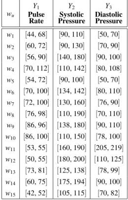
Table 3.Blood Dataset.
To illustrate, take the blood data of Table 3 (taken from Billard and Diday, 2006, Table 3.5). Here,Y1=pulse rate,Y2=systolic
pres-sure, and Y3 = diastolic pressure. These data
may have arisen by aggregating values for in-dividuals making up the respective categories Ω ={w1,· · ·,w15}. Or, since it is known that
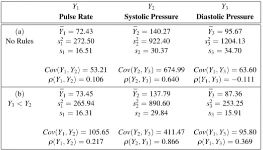
pulse rates and blood pressure values typically fluctuate considerably, the categories{wu}can be measurements over time on single individ-uals. The sample mean and variance for each variable obtained from(1) and (2), as well as the covariances from(6)and hence the correla-tion funccorrela-tions, are shown in Table 4(a).
It is often the case that logical dependency rules exist to maintain the integrity of the data and/or to perform the role of data cleaning. Here, since diastolic pressure is less than systolic pressure, Y3 < Y2, the observationw11, by violating this
axiom, should be omitted as a data cleaning ex-ercise. The resulting sample means, variances, covariances and correlations are given in Ta-ble 4(b). In this case, the Y2 and Y3 values
are such that all Y3/Y2 values violate the rule
ν :Y3<Y2. More generally, aggregation of
in-dividual values, each of which has Y3 < Y2,
Y1 Y2 Y3
Pulse Rate Systolic Pressure Diastolic Pressure
(a) Y1¯ =72.43 Y2¯ =140.27 Y3¯ =95.67 No Rules s2
1 =272.50 s22=922.40 s23=1204.13 s1=16.51 s2=30.37 s3=34.70 Cov(Y1,Y2) =53.21 Cov(Y2,Y3) =674.99 Cov(Y1,Y3) =63.60
ρ(Y1,Y2) =0.106 ρ(Y2,Y3) =0.640 ρ(Y1,Y3) =−0.111
(b) Y¯1 =73.45 Y¯2=137.79 Y¯3=87.36 Y3<Y2 s2
1 =265.94 s22=890.60 s23=253.25 s1=16.31 s2=29.84 s3=15.91 Cov(Y1,Y2) =105.65 Cov(Y2,Y3) =411.47 Cov(Y1,Y3) =95.80
ρ(Y1,Y2) =0.217 ρ(Y2,Y3) =0.866 ρ(Y1,Y3) =0.369
Table 4.Descriptive Statistics.
(Y2,Y3) = ([160,190],[170,185]), say. Now,
only that portion bounded by the vertices(160, 170),(160, 185),(185, 185),(170, 170) form-ing a hexagon in R2 is a valid region. This is
analogous to the baseball dataset analysed in detail in Billard and Diday(2006), q.v.
3. Principal Component Analysis
Chouakria(1998)and Billard et al. (2008)have proposed a principal component methodology based on the vertices of the data hypercubes. They show that theνth symbolic principal com-ponent is
Yu∗ν = [yauν,ybuν], ν =1, . . . ,s≤p, (7) where
yauν = min
k∈Lu{y
u
νk}, ybuν =maxk∈L
u{y
u
νk} (8)
where yuνk is the νth principal component for the vertexkof the hypercube of observationwu
andLuis the set of vertices associated withwu.
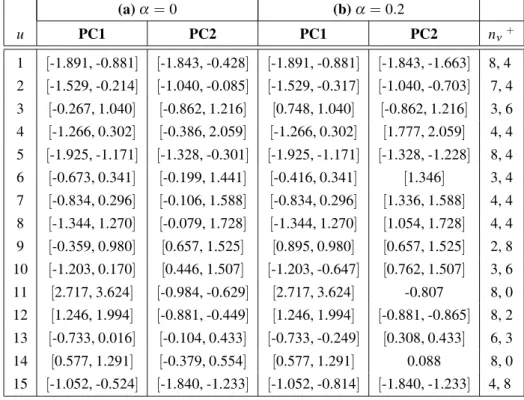
The resultingν = 1 and ν = 2 principal com-ponents PCν for the blood data of Table 3 are shown in Table 5(a)and plotted in Figure 1. In order to help clarify the visualization and in-terpretation of these principal components, it is further proposed to retain for use in (8) only those verticesxuk whose contribution
Ctr(xik,PCν) = [d((xyiνik)2
k,G)]2
exceeds a specified α. In (9), xuk is the vertex k inLu, d(·,G)is the Euclidean distance from
that vertex and the centroid G of all observa-tions. Eqn (8)directly corresponds to α = 0. Whenα =0.2, the principal componentsPCν, ν = 1,2, are as shown in Table 5(b); the num-ber of vertices nν which satisfies this condi-tion, ν = 1,2, is also shown. The resulting PCν,ν =1,2, are plotted in Figure 2.
The clusters become more apparent in Figure 2. Thus, we see that observations{w1,w2,w5,w15}
=C1constitute one cluster;{w4,w6,w7,w8,w9,
w10} = C2 form a second cluster, with maybe
w13part of this second cluster if not its own
clus-ter; {w3,w12,w14} are a single cluster C3 (or
perhaps two clusters); and finally{w11} = C4
is a cluster on its own.
Figure 3 is the plot of thePC1 andPC2 obtained when the interval midpoints are used as classi-cal surrogates. Unlike the distinctness of w3
and w14 in the symbolic analysis, these
obser-vations would seem to be part of the central clus-terC2. The degree of these differences depends
on the varied lengths of the intervals. More importantly, however, the relative sizes of the principal component hypercubes reflect those of the data hypercubes. For example, compar-ing those for w3 and w14 in Figure 1 (or in
Figure 4 below), we see how the data hyper-cube forw4 fits “inside” that ofw14 as do also
Figure 1.
Figure 3.
(a)α =0 (b)α =0.2
u PC1 PC2 PC1 PC2 nν+
1 [-1.891, -0.881] [-1.843, -0.428] [-1.891, -0.881] [-1.843, -1.663] 8, 4 2 [-1.529, -0.214] [-1.040, -0.085] [-1.529, -0.317] [-1.040, -0.703] 7, 4 3 [-0.267, 1.040] [-0.862, 1.216] [0.748, 1.040] [-0.862, 1.216] 3, 6 4 [-1.266, 0.302] [-0.386, 2.059] [-1.266, 0.302] [1.777, 2.059] 4, 4 5 [-1.925, -1.171] [-1.328, -0.301] [-1.925, -1.171] [-1.328, -1.228] 8, 4 6 [-0.673, 0.341] [-0.199, 1.441] [-0.416, 0.341] [1.346] 3, 4 7 [-0.834, 0.296] [-0.106, 1.588] [-0.834, 0.296] [1.336, 1.588] 4, 4 8 [-1.344, 1.270] [-0.079, 1.728] [-1.344, 1.270] [1.054, 1.728] 4, 4 9 [-0.359, 0.980] [0.657, 1.525] [0.895, 0.980] [0.657, 1.525] 2, 8 10 [-1.203, 0.170] [0.446, 1.507] [-1.203, -0.647] [0.762, 1.507] 3, 6 11 [2.717, 3.624] [-0.984, -0.629] [2.717, 3.624] -0.807 8, 0 12 [1.246, 1.994] [-0.881, -0.449] [1.246, 1.994] [-0.881, -0.865] 8, 2 13 [-0.733, 0.016] [-0.104, 0.433] [-0.733, -0.249] [0.308, 0.433] 6, 3 14 [0.577, 1.291] [-0.379, 0.554] [0.577, 1.291] 0.088 8, 0 15 [-1.052, -0.524] [-1.840, -1.233] [-1.052, -0.814] [-1.840, -1.233] 4, 8
+nν=# of vertices retained
Table 5.Principal Components.
α =0.2
u PC1 PC2 nν
1 [-2.838, -1.302] [-1.149, -1.149] 8, 1 2 [-1.833, -0.836] [-0.662, -0.662] 6, 1 3 [0.402, 1.579] [-1.370, 0.777] 5, 6 4 [-0.896, 1.469] [1.738, 2.229] 4, 4 5 [-2.677, -1.439] 0.022 8, 0 6 [-0.414, 1.351] [1.113, 1.414] 6, 4 7 [-0.612, 0.964] [1.115, 1.479] 3, 4 8 [-1.174, 2.282] [1.285, 1.595] 4, 2 9 [0.297, 2.049] [0.591, 1.099] 7, 3 10 [-0.713, 1.138] [0.582, 1.635] 3, 7 12 [1.309, 2.352] [-2.039, -1.498] 8, 8 13 [-0.622, 0.553] [0.378, 0.541] 5, 3 14 [0.622, 1.619] [-1.286, -1.046] 8, 4 15 [-1.821, -1.011] [-1.386, -0.785] 8, 7
Table 6.Principal Components,Y3 <Y2.
Finally, under the rule ν : Y3 < Y2, the
sym-bolic principal components PCν, ν = 1,2 for α =0.2 are shown in Table 6 and plotted in Fig-ure 4. The effect of the invalid datapoint w11
is immediately apparent by comparing Figure 2 and Figure 4.
4. Clusters
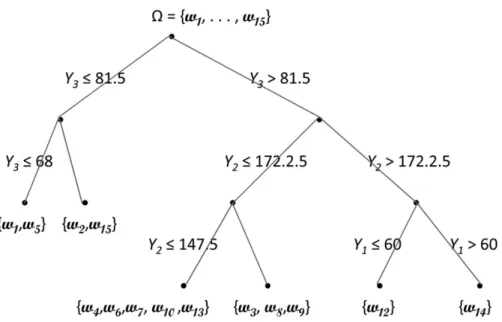
As another example of the distinctness of a sym-bolic analysis over a classical analysis, the divi-sive clustering method of Chavent(1997, 1998, 2000)is applied to the symbolic data in Table 3, under the ruleY3 <Y2. The resulting hierarchy
Figure 5.Divisive clustering on symbolic data,Y3<Y2.
Figure 6.Divisive clustering on classical midpoints,Y3<Y2.
5. Conclusion
With the advent of the modern computer, large datasets are ubiquitous. Aggregation across cat-egories in these large datasets will inevitably produce symbolic data. Therefore, it is
References
[1] P. BERTRAND, F. GOUPIL, Descriptive statistics for
symbolic data. In: Analysis of Symbolic Data: Exploratory Methods for Extracting Statistical In-formation from Complex Data (eds. H.-H. Bock and E. Diday). Springer-Verlag, Berlin, (2000), 103–124.
[2] L. BILLARD, Dependencies and variation compo-nents of interval-valued data. In: Selected Contri-butions in Data Analysis and Classification(eds. P. Brito, P. Bertrand, G. Cucumel and F. de Carvalho), Springer,(2007), 3–12.
[3] L. BILLARD, A. CHOUAKRIA-DOUZAL, E. DIDAY,
Symbolic principal components for interval-valued observations,(2007).
[4] L. BILLARD, E. DIDAY, Symbolic Data Analysis:
Conceptual Statistics and Data Mining, (2006). John Wiley.
[5] L. BILLARD, E. DIDAY, Descriptive statistics for
interval-valued observations in the presence of rules. Computational Statistics. 21,(2006), 187–210.
[6] M. CHAVENT, Analyse de Donne´es Symboliques
Une M´ethode Divisive de Classification, Th´ese de Doctorat, Universit´e Paris Dauphine,(1997).
[7] M. CHAVENT, A monothetic clustering algorithm. Pattern Recognition Letters19,(1998), 989–996.
[8] M. CHAVENT, Criterion-based divisive clustering for symbolic data. In: Analysis of Symbolic Data: Exploratory Methods for Extracting Statistical In-formation from Complex Data (eds. H.-H. Bock and E. Diday). Springer-Verlag, Berlin, (2000), 299–311.
[9] A. CHOUAKRIA,Extension des M´ethodes d’analyse
Factorielle a des Donn´ees de Type Intervale, Th´ese de Doctorat, Universit´e Paris, Dauphine,(1998).
[10] E. DIDAY, M. NOIRHOMME-FRAITURE, (EDS.)
Sym-bolic Data Analysis and the SODAS Software,
(2008). Wiley.
Received:June, 2008
Accepted:September, 2008
Contact address:
Lynne Billard Department of Statistics University of Georgia Athens, GA 30602, USA e-mail:[email protected]