Volume 13, Issue 1, January 2016 · Econ Journal Watch

Scholarly Comments on Academic Economics

ECONOMICSIN PRACTICE

INVESTIGATINGTHE APPARATUS

CHARACTER ISSUES

Editor’s Notes: Acknowledgments 2014–15 1–4

A Unit Root in Postwar U.S. Real GDP Still Cannot Be Rejected, and Yes, It Matters

David O. Cushman 5–45

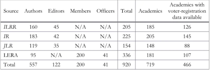
The Left Orientation of Industrial Relations

Mitchell Langbert 46–74

Eli Heckscher’s Ideological Migration Toward Market Liberalism

Benny Carlson 75–99

SYMPOSIUM

SYMPOSIUM

CLASSICAL LIBERALISMIN ECON, BY COUNTRY (PART III)

Liberalism in Korea

Young Back Choi and Yong J. Yoon 100–128

Liberalism in Mexican Economic Thought, Past and Present

WATCHPAD

Foreword to “Glimpses of Adam Smith”

Daniel B. Klein 168

Glimpses of Adam Smith: Excerpts from the Biography by Ian Simpson Ross

Editor’s Notes:

Acknowledgments 2014–15

I thank co-editors Garett Jones, George Selgin, and Larry White for their fine work, and Bruce Benson and Fred Foldvary, who are now co-editors emeriti. The managing editor Jason Briggeman not only continues to do an astounding job in improving every piece we publish, by copy-editing, fact-checking, and ensuring accuracy throughout every reference and virtually every detail, but also in advising on refashioning papers in structure and substance, and on what to select for publi-cation. Jason’s excellence and commitment to the project is crucial to whatever success it enjoys.

We are grateful to Jane Shaw Stroup, who has helped greatly with many manuscripts, in particular many of the pieces (twelve, and counting) for the

symposium “Classical Liberalism in Econ, by Country.” We also thank Kurt Schuler, for his guidance and ideas. We are grateful to web virtuoso John Stephens for continuing to fine-tune the superb website and document-production system that he created, and to Ryan Daza, Eric Hammer, and Erik Matson for occasional service to the journal.

For friendship and vital sponsorship over the past two years, we are grateful to donors. From the start of EJW, the project has enjoyed faithful and generous support from the Earhart Foundation, which has now come to the end of its mission. Like many others, EJW will always remember and be grateful for Earhart’s friendship and beneficence. For support we also thank the Charles G. Koch Foundation, Gerry Ohrstrom, and the John William Pope Foundation. I am very grateful to Rich and Mary Fink and the Fink family, for the generous Mercatus Center JIN chair (“JIN” for three of the family’s beloved), which I hold and that helps to support EJW.

We are ever deeply grateful to Atlas Network, for housing EJW within their organization and for their friendship and utterly in-kind support (accounts, pay-ments, reporting, etc.), especially Romulo Lopez, Harry Kalsted, Brad Lips, and Alejandro Chafuen.

for asymposiumon economists on the welfare state and the regulatory state, in particular Claire Morgan for facilitating the collaboration and organizing anevent

at Mercatus in connection with the symposium.

We are grateful to our authors, for generously contributing their creativity, craftsmanship, and industriousness, as well as for their patience and cooperation in our editorial process.

The “Classical Liberalism in Econ, by Country”authorsshould be thanked in particular for their courage in standing up for liberal causes, often under pro-fessional and ideological adversity, some under conditions of personal danger to themselves and their family.

We thank the following individuals for generously providing intellectual accountability to EJW:

Referees during 2014–15

Sarah Babb Boston College

James T. Bennett George Mason University Jagdish Bhagwati Columbia University Charles Ballard Michigan State University

Chris Berg RMIT University, Melbourne

Robert Ciborowski University of Białystok

John Cochrane Hoover Institution, Stanford University William Coleman Australian National University

Tyler Cowen George Mason University

David O. Cushman Westminster College (Pennsylvania) Charles de Bartolomé University of Colorado, Boulder Bryan Caplan George Mason University Shikha Sood Dalmia Reason Foundation

Michael Davis Missouri University of Science and Technology Maren Duvendack University of East Anglia

Hugo Faria University of Miami

Amihai Glazer University of California, Irvine

Robin Grier University of Oklahoma

Michael Hadani Saint Mary College of California James Hamilton University of California, San Diego

Eric Hammer George Mason University

Mark Hanssen Catholic University

Björn Hasselgren Royal Institute of Technology (Sweden) Philip Hersch Wichita State University

Fergus Hodgson PanAm Post

Jeffrey Rogers Hummel California State University, San Jose

Dragan Ilić University of Basel

William Jeynes California State University, Long Beach

April Kelly-Woessner Elizabethtown College

Chung-Ho Kim Yonsei University

Arnold Kling Mercatus Center, George Mason University

Mark Koyama George Mason University

Pravin Krishna Johns Hopkins University Pavel Kuchař University of Guanajuato Ashish Lall National University of Singapore Cesar A. Martinelli George Mason University James McClure Ball State University Bruce McCullough Drexel University Brian Meehan Florida State University

Boško Mijatović Center for Liberal-Democratic Studies Jeffrey Milyo University of Missouri

Carl Moody College of William & Mary

Adrian Moore Reason Foundation

Steven Mullins Drury University Peter Nedergaard University of Copenhagen

Martin Paldam Aarhus University

Svetozar Pejovich Texas A&M University Marta Podemska-Mikluch Gustavus Adolphus College Danica Popović University of Belgrade John Quiggin University of Queensland Suri Ratnapala University of Queensland Pedro Romero Universidad San Francisco de Quito

Paul Rubin Emory University

Christos Sakellariou Nanyang Technical University Walter Schumm Kansas State University Jane Shaw Stroup John William Pope Foundation Slaviša Tasić University of Mary

Ian Vasquez Cato Institute

Gary Walton University of California, Davis Glen Whitman California State University, Northridge Michael Wolf University of Zurich

Todd Zywicki George Mason University

Commented-on authors replying in EJW, published 2014–15

Laura Langbein American University (article link)

John A. List University of Chicago (article link)

Zacharias Maniadis University of Southampton (article link)

Fabio Tufano University of Nottingham (article link)

Other individuals who published commentary on EJW material in EJW, published 2014–15

Olav Bjerkholt University of Oslo (article link)

Ib E. Eriksen University of Agder (article link)

Robert Kadar Evolution Institute (article link)

Steve Roth Independent researcher (article link)

Arild Sæther University of Agder (article link)

Lawrence H. White George Mason University (article link)

David Sloan Wilson State University of New York at Binghamton (article link)

A Unit Root in Postwar U.S. Real

GDP Still Cannot Be Rejected,

and Yes, It Matters

David O. Cushman

LINKTO ABSTRACT

Does real gross domestic product (GDP) have an autoregressive unit root or is it trend stationary, perhaps with very occasional trend breaks? If real GDP has an autoregressive unit root, then at least a portion of each time period’s shock to real GDP is permanent. Booms and recessions therefore permanently change the future path of real GDP. But if real GDP is trend stationary, (almost all) shocks to real GDP are transitory, and real GDP (almost always) reverts to an already existing trend.2

Here I present evidence that, despite the findings or implications of some recent papers and blog entries, the hypothesis of a unit root in U.S. real GDP after World War II cannot be rejected, once the issues of individual and multiple-test size distortion are dealt with. But are the implied permanent shocks important relative to transitory shocks? They are, according to an unobserved components model and a vector error correction model (VECM) proposed by John Cochrane (1994). Moreover, permanent shocks have strong effects according to impulse response analysis of the Cochrane VECM. Finally, models with unit roots forecast better over the postwar period than trend stationary models. This is particularly true for forecasts of recoveries from seven postwar recessions, and Cochrane’s VECM, with its specific identification of permanent and transitory shocks, performs best ECON JOURNAL WATCH 13(1) January 2016: 5–45

1. Westminster College, New Wilmington, PA 16172; University of Saskatchewan, Saskatoon, SK S7N 5A5, Canada.

overall. Thus, by every measure the unit root has “oomph,” as Stephen Ziliak and Deirdre McCloskey would say.3

Background

In a landmark paper, Charles Nelson and Charles Plosser (1982) argued against the then-prevailing assumption (noted by Stock and Watson 1999) of trend stationarity for U.S. real GDP. Nelson and Plosser showed that the unit root could not be rejected in favor of trend stationarity. Their claim has led to a large number of papers examining the issue with a variety of tests, specifications, data periods, and countries. For U.S. real GDP, James Stock and Mark Watson (1999) judged that the unit root testing literature supported Nelson and Plosser’s (1982) conclu-sion. More recently, Spencer Krane (2011) concluded that the Blue Chip Consensus real GDP forecasts have important permanent components. Sinchan Mitra and Tara Sinclair (2012) stated that “fluctuations in [U.S. real GDP] are primarily due to permanent movements.” But other papers since Stock and Watson’s (1999) judgment have claimed that the unit rootcanbe rejected (see, e.g., Ben-David, Lumsdaine, and Papell 2003; Papell and Prodan 2004; Vougas 2007; Beechey and Österholm 2008; Cook 2008; Shelley and Wallace 2011).

In recent years, the unit root-GDP issue has made lively appearances in in economics blogs. Greg Mankiw (2009a) argued that the likely presence of a unit root cast doubt on the incoming Obama administration’s 2009 forecast of strong recovery (Council of Economic Advisers 2009). Brad DeLong (2009) and Paul Krugman (2009) immediately disputed Mankiw’s invocation of a unit root as cause for pessimism, arguing that the shocks that generated the 2008–09 recession were transitory, although Krugman allowed that shocks could occasionally be per-manent (Cushman 2012; 2013). In commenting on the Mankiw-DeLong-Krugman controversy, Menzie Chinn (2009) ran an econometric test that rejected the unit root. Stephen Gordon (2009), responding in turn to “DeLong-Krugman-Mankiw-Chinn,” said: “There’s little evidence that we should be operating under the unit-root hypothesis during recessions. Or during expansions, come to that.” He provocatively followed this with: “The world would be a better place if…the whole unit root literature never existed.”

Cochrane (2012) wrote that “the economy has quite reliably returned to the trend line after recessions,” providing a GDP graph with a trend line fitted over 1967–2007. This claim seems to support the trend stationarity hypothesis. But Cochrane has believed for some time that GDP has a unit root (Cochrane 1994;

3.SeeZiliak and McCloskey 2008; McCloskey and Ziliak 2012.

2015a). The Cochrane (2012) graph may be a dramatic illustration of the blog entry’s title (“Just How Bad Is the Economy?”) and reflect a belief that shocks causing recessions were mostly transitory prior to 2007. Cochrane’s blog entry cited John Taylor (2012), who wrote (citing in turn Bordo and Haubrich 2012) that “deep recessions have always been followed by strong rather than weak recoveries.” Similarly, Marcus Nunes (2013) presented a graph that looks like a linear trend stationary model with a break in 2008 from a one-time shock that is permanent and transitory in roughly equal proportions. Nevertheless, although Taylor’s presen-tation and certainly Nunes’s are suggestive of the trend spresen-tationary hypothesis, Taylor and Nunes did not mention unit roots or stationarity, and so it is not clear what, if anything, they may have believed about the issue. Meanwhile, William Easterly (2012) wrote, facetiously, that the unit root question could be a factor in the 2012 U.S. presidential election, because a unit root in output could be seen as relieving President Obama of blame for the weak recovery. Scott Sumner (2014) pointed out that Mankiw’s (2009a; 2009b) unit root-based skepticism about re-covery by 2013 had been confirmed.4

Quite recently, Roger Farmer (2015) applied a unit root test to U.S. real GDP 1955:2–2014:1. The result was a clear failure to reject the unit root. Farmer concluded: “There is no evidence that the economy is self-correcting.”5_Arnold

Kling (2015) used Farmer’s result to argue that “the concept of potential GDP can have no objective basis.” In contrast, John Taylor (2015) reprinted a graph (from Taylor 2014) showing a linear trend based on the 2001–2007 GDP growth rate that extends through 2024, a trend which he argued could be reached if certain policies are followed. This looks like trend stationarity. Finally, Larry Summers (2015) wrote that for “over 100 recessions [in] industrial countries over the last 50 years…in the vast majority of cases output never returns to previous trends” (referring to Blanchard, Cerutti, and Summers 2015). This implies a unit root.

Thus, seventeen years after Stock and Watson’s (1999) judgment about GDP and unit roots, the issue remains controversial.

A summary of what I do and find

I start by analyzing whether the recent unit root rejections in the academic literature (and one in a blog), when combined with earlier rejections, are numerous or strong enough to overturn the 1999 Stock-Watson assessment in favor of unit roots in postwar real GDP. I implement corrections for two problems that cast doubt on the various existing rejections of the unit root in real GDP:

1. Size distortion in individual unit root tests: the tendency of a test to reject at rates exceeding the stated significance level when the null is actually true. The distortion results from the pre-testing for lag order and from the magnitude of the lag parameters, and has seldom been addressed in papers that reject the unit root in real GDP.

2. The multiple-test problem: what to decide when some tests reject but others do not, while maintaining the stated significance level. This has not been addressed in any papers on the GDP/unit root question.

For problem (1), I use bootstrapped distributions to get size-adjusted p -values for individual tests. For problem (2), I use the bootstrapped distributions to get several variations of size-adjusted jointp-values for various sets of unit root tests. The most comprehensive jointp-values show no rejections at the 0.05 level, and hardly any at the 0.10 level. I thus conclude that the unit root null cannot be rejected.

I then turn to the question of the economic importance of the unit root. The question matters because the unit root could be dominated by a transitory component, rendering its statistical significance economically unimportant. I there-fore compute indicators of the relative importance of permanent shocks using an unobserved components approach, as in Krane (2011) and Mitra and Sinclair (2012), and the vector error correction approach of Cochrane (1994). The esti-mates of permanent shocks are economically significant.

Finally, I examine how allowing for unit roots would have affected forecasts of real GDP in the postwar period. Lawrence Christiano and Martin Eichenbaum (1990) and Cochrane (1991a; 1991b) pointed out that a unit root process could be very closely approximated by a stationary process. Nevertheless, I find that specifying a unit root usually does improve forecasts, particularly after recessions. The advantage is most consistent using Cochrane’s (1994) VECM that separately identifies both transitory and permanent shocks.

The unit root test literature on

postwar U.S. real GDP, and its interpretation

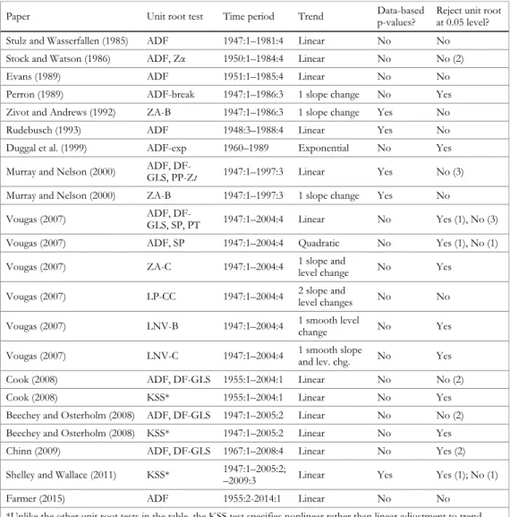
Table 1 lists papers over the last 31 years that have applied unit root tests to postwar U.S. real GDP.6The null hypothesis in these papers is that a unit root is present. I am unaware of any papers in peer-reviewed journals focusing on U.S. real GDP for which trend stationarity is the null.7_{This is consistent with a sentiment,}

attributed to Bennett McCallum, that “it seems strange that anything could be trend stationary” (see McCallum 1991).

In indicating the unit root rejections in Table 1, I have corrected two er-roneous interpretations by Vougas (2007). He reported that his PT and LP-CC test values rejected the unit root, but he apparently misinterpreted the tests’ rejection regions; the two results are not rejections. See Appendix 1 for details. I use the correct interpretation for the two tests because I don’t want my assessment of the prevalence of unit root rejections affected by this problem.

In Table 1 there are 33 test results reported, and 12 (36 percent) reject the unit root at the 0.05 level.8_{The table also presents the state of affairs regarding several}

issues that could affect test outcome or validity:

1. Data period: Tests with more data will, ceteris paribus, have more power.

2. Trend specification: A simple linear trend (under alternative hypothesis of stationarity) has been the most common specification, but some tests have specified trends with breaks to allow for infrequent perma-nent shocks. Other tests have specified nonlinear trends to allow for gradual evolutions in growth rates. If stationarity is the case and real GDP has a breaking or nonlinear trend, then a test that correctly speci-fies the trend will tend to have more power, although estimating the extra trend parameters tends to offset the power gain.

6. I do not include the few papers that have tested for a unit root in U.S. per capita real GDP (e.g., Stock and Watson 1986; Cheung and Chinn 1997), only in real GDP itself, the more common approach. The table contains standard journal articles with two exceptions, Chinn (2009) and Farmer (2015), which are blog entries. One might not want to include work found in blogs because blogs are not vetted for their econometrics as refereed journal articles normally are. But in this case I include the blog entries as an illustration of the continued interest in applying unit root tests to GDP, and because Chinn and Farmer are highly respected scholars.

7. Cheung and Chinn (1997) test the null of trend stationarity in postwarper capitareal GNP. Chinn (2009) and Farmer (2015) apply the KPSS test in their blogs.

3. The adjustment process: The KSS test, applied three times, features nonlinear adjustment. With traditional, so-called ‘linear’ adjustment specified in a test, then—under stationarity and in the absence of further shocks—a constant fraction of the deviation from the long-run trend is assumed to be eliminated in each time period. The more recent KSS approach is to specify ‘nonlinear’ adjustment in unit root tests. With nonlinear adjustment, the fraction of the deviation from trend that is eliminated is assumedlargerwhen the variable is far from the trend than when it is close. The motivation to model real GDP this way, as given by Meredith Beechey and Pär Österholm (2008), is that the central bank would be likely to respond disproportionately more strongly to significant inflationary booms and recessions than to small fluctuations. If, under stationarity, adjustment is indeed nonlinear and the test’s specification of the nonlinear adjustment is reasonably accurate, then the test could have higher power.

4. Sampling distributions: Christian Murray and Charles Nelson (2000) emphasized that unit root tests were likely to suffer from size distor-tion: excessive rejections under the null, because of data heterogeneity and data-based lag selection. The lag selection issue is that unit root tests often require an autoregressive lag order choice, which is usually based on the same data as used for the test itself. G. William Schwert (1989) and Glenn Rudebusch (1993) discussed another problem: the ef-fect of specific serial correlation parameter values of relevant sign and/ or sufficient magnitude. Murray and Nelson’s (2000) response was, in addition to using only postwar data, to employ data-based sampling distributions—bootstrapping—and to include the lag choice decision process in the bootstrapping. Schwert (1989), Rudebusch (1993), and Eric Zivot and Donald Andrews (1992) had also previously used data-based sampling distributions to address size distortion.

In Table 1, the reported unit root rejections tend to be associated with more recent papers having longer data sets (10 of the 12 test rejections are in papers published after 2000), with specifications including breaking or nonlinear trends, and/or with specifications with nonlinear adjustment to trend. However, with just one exception the rejections also come from sampling distributions that are not data-based. So, do the rejections reflect higher power from longer data sets and better trend or adjustment specifications, or do the rejections just reflect size distortion from using non-data-based distributions?

TABLE 1. Various papers and their unit root conclusions

Paper Unit root test Time period Trend Data-based_p-values? Reject unit root_{at 0.05 level?}

Stulz and Wasserfallen (1985) ADF 1947:1–1981:4 Linear No No

Stock and Watson (1986) ADF, Zα 1950:1–1984:4 Linear No No (2)

Evans (1989) ADF 1951:1–1985:4 Linear No No

Perron (1989) ADF-break 1947:1–1986:3 1 slope change No Yes

Zivot and Andrews (1992) ZA-B 1947:1–1986:3 1 slope change Yes No

Rudebusch (1993) ADF 1948:3–1988:4 Linear Yes No

Duggal et al. (1999) ADF-exp 1960–1989 Exponential No Yes

Murray and Nelson (2000) ADF, DF-_{GLS, PP-Zt} 1947:1–1997:3 Linear Yes No (3)

Murray and Nelson (2000) ZA-B 1947:1–1997:3 1 slope change Yes No

Vougas (2007) ADF, DF-_{GLS, SP, PT} 1947:1–2004:4 Linear No Yes (1), No (3)

Vougas (2007) ADF, SP 1947:1–2004:4 Quadratic No Yes (1), No (1)

Vougas (2007) ZA-C 1947:1–2004:4 1 slope and_{level change} No Yes

Vougas (2007) LP-CC 1947:1–2004:4 2 slope and_{level changes} No No

Vougas (2007) LNV-B 1947:1–2004:4 1 smooth level_change No Yes

Vougas (2007) LNV-C 1947:1–2004:4 1 smooth slope_{and lev. chg.} No Yes

Cook (2008) ADF, DF-GLS 1955:1–2004:1 Linear No No (2)

Cook (2008) KSS* 1955:1–2004:1 Linear No Yes

Beechey and Osterholm (2008) ADF, DF-GLS 1947:1–2005:2 Linear No No (2)

Beechey and Osterholm (2008) KSS* 1947:1–2005:2 Linear No Yes

Chinn (2009) ADF, DF-GLS 1967:1–2008:4 Linear No Yes (2)

Shelley and Wallace (2011) KSS* 1947:1–2005:2;_–2009:3 Linear Yes Yes (1); No (1)

Farmer (2015) ADF 1955:2-2014:1 Linear No No

*Unlike the other unit root tests in the table, the KSS test specifies nonlinear rather than linear adjustment to trend under the trend stationary alternative hypothesis.

Test definitions and sources:

ADF = augmented Dickey-Fuller test with linear or quadratic trend (Ouliaris et al. 1989) ADF-exp = ADF test with exponential trend (Duggal et al. 1999)

ADF-break = ADF test of residuals of the regression ofyon a trend with a slope change at a known date (Perron 1989) DF-GLS = modified ADF test of Elliott et al. (1996) with linear or quadratic trend

KSS = Kapetanios et al. (2003) test with linear trend

LNV-B, LNV-C = Leybourne et al. (1998) test, models B and C LP-CC = Lumsdaine and Papell (1997) test, model CC PP-Zt= Phillips and Perron (1988) Z(t) test with a linear trend PT = Point optimal test of Elliott et al. (1996) with linear trend

SP = Schmidt and Phillips (1992) tau test with linear trend or quadratic trend Zα = Phillips (1987) Zα test modified with assumed trend

There is another issue, however, for which the table does not present dence. Is the rejection by 36 percent of tests, as in Table 1, sufficiently strong evi-dence against the unit root for an overall rejection? When a null is true and many tests are applied either by one researcher or by many, getting at least one rejection becomes increasingly likely. The overall significance of results such as in Table 1 is thus unknown without further work. The problem is a version of the classic multiple test problem, which is the problem of getting correct significance levels when there are many tests using a single sample (see on this Romano et al. 2010).

Suppose 10 tests of the unit root null are applied to a data set (as in Vougas 2007). If, under the null, the 10 tests are uncorrelated with each other, then we will observe one or more rejections not 5 percent of the time, the nominal level of significance, but 40 percent of the time (from the binomial distribution). And when we get rejections, there will be two or more 21 percent of the time. But the unit root test results are hardly uncorrelated because they are applied to the same data set.

For a concrete example, suppose the correlation for each test pair (with 10 tests, there are 45 pairs) under the null is 0.80 and the individual test statistics happen to be standard normal. Then the probability of getting one or more rejec-tions falls to 16 percent, but this still exceeds 5 percent. Moreover, if we get any rejections in this case, there will now be two or more about 40 percent of the time. And there will be four rejections (approximately the proportion in Table 1) or more 33 percent of the time. Overall, under the null, observing more than one rejection among 10 tests with a probability significantly exceeding the stated 5 percent significance level is quite likely.9

Unit root tests with the above issues addressed

I apply a large number of previously used unit root tests and variations, 42 tests in all. The same estimation period is used for all, so different conclusions from the tests do not reflect different time periods.10To account for individual-test size distortion, I employ a bootstrap approach using five data-generating processes (DGPs). To account for the multiple test problem, for each DGP I compute joint p-values in four ways for all 42 tests and several subsets. And then I compute overall jointp-values of the four joint p-values for the various subsets. Finally, because results differ among the DGPs, I try several ways of weighting the DGPs’ jointp -values to yield an overallp-value for each group of tests using eachp-value method.

9. Under independence, the probabilities can be calculated using the binomial distribution. For the correlated case, the probabilities are estimated with 40,000 replications assuming a multivariate normal distribution for the test statistics.

10. Generally, TSP 5.1 is used for econometric computations in the paper. Exceptions are noted below.

Data set

The data sets in most papers in Table 1 start in 1947:1 (or not too long thereafter) and end shortly before the paper was written, and I could follow this pattern. But Gary Shelley and Frederick Wallace (2011) find no rejections, contrary to Beechey and Österholm (2008), when the data are extended to include the 2008–2009 recession. Farmer’s (2015) data also includes the recession, and he reports non-rejection. This could reflect a permanent shock to a generally trend stationary real GDP. Such a break adds a challenge to the rejection of the unit root (supposing it should be rejected) that earlier papers did not face. But I do not want my critique to be influenced by this problem. Therefore, my data set starts in 1947:1 and ends not with the most recent data available to me, but in 2007:3, just before the recession’s start in 2007:4.11

The unit root tests

I employ all the tests and trend specifications in Table 1, but with a few changes. Regarding trends, I omit one and add one. The omitted trend is the expo-nential trend of Vijaya Duggal, Cynthia Saltzman, and Lawrence Klein (1999), who included the term exp(tΦ_{) as the (only) deterministic term in an ADF test. But the}

estimated trend curvature and the unit root test result are then dependent on setting the initial date fortequal to 1. An exponential trend without this defect is used by Robert Barro and Xavier Sala-i-Martin (1992), but there is no unit root test with this trend. For postwar U.S. real GDP, however, the Barro and Sala-i-Martin (1992) exponential trend and the quadratic trend are almost identical, so the unit root tests with a quadratic trend approximate the Barro and Sala-i-Martin trend.12

The trend I add has two slope changeswithout level changes. This extends the Zivot and Andrews (1992) one-slope-change model B to the two-slope-change case and is therefore like the Robin Lumsdaine and David Papell (1997) model CC but with no level changes. I label the result ZA-LP. Thus, we now have one-and two-slope-change tests both with level changes and without them.

The additional adjustments to the Table 1 tests are the following. First, in-stead of Stock and Watson’s (1986) inclusion of an assumed trend in Peter Phillips’s (1987) Zα test, I follow Phillips and Pierre Perron’s (1988) inclusion of an estimated trend. I label the latter version PP-Zα. The second adjustment is to substitute the superior DF-GLS test for the regular ADF test in the case of the quadratic

trend, and the third is to substitute the modified feasible point optimal test (MPT) from Serena Ng and Pierre Perron (2001) for the unmodified version (PT) of Graham Elliott, Thomas Rothenberg, and James Stock (1996).13Next, I do not use Perron’s (1989) known-breakpoint approach, only the Zivot and Andrews (1992) estimated-breakpoint version, ZA-B. And, because the unit root rejections in Table 1 for the three KSS applications with a simple linear trend suggest relevance for nonlinear adjustment, I add tests with KSS nonlinear adjustment for all other trend specifications.14

To adjust for serial correlation, the tests in Table 1 almost always use auto-regressive lags. The most common method for lag order choice is the AIC, followed by the BIC and the Ng and Perron (1995) recursive test-down. Steven Cook (2008) simply employs the same lag order every time. Consistent with accounting for many test procedures, I try both the AIC (or the Ng and Perron 2001 modification, MAIC) and BIC for all autoregressive cases. But time is limited so I omit the test-down and fixed-lag approaches. The exceptions in Table 1 to using autoregressive lags are the nonparametric approaches in the Zα, PP-Zα, and PP-Zt tests and in Vougas’s (2007) implementation of the PT test. I use the standard PP-Zα and PP-Zttests but, because I replace the PT test with the MPT test, I follow Ng and Perron’s (2001) use of autoregressive lags for the MPT test. And I use the MAIC for the DF-GLS and MPT tests as in Ng and Perron (2001).

In choosing the lag, the maximum considered is usually 14, frommaxlag= Int[12(T/100)0.25_{] (Schwert 1989) whereT= 243, the sample size. The exceptions} are the tests from Peter Schmidt and Peter Phillips (1992). With linear trend,maxlag = 14 gives lag order 1, not 2 as in Vougas (2007), and then the unit root is not rejected, unlike in Vougas (2007). Perhaps he used a smallermaxlag. Withmaxlag= 12, I get his result. I do not want my critique of unit root rejections to be affected by this minor distinction, and so for the Schmidt-Phillips tests I setmaxlag= 12.15

Bootstrapping and exact

pp

-value procedure for the individual

tests

I compute individual testp-values using a wild bootstrap that adjusts for size distortion from the specific lag coefficients in DGPs and heteroskedasticity from the Great Moderation, viz., the reduction in real GDP variance from 1984 onwards

13. Cushman (2002) is the first I know of to include a quadratic trend in the DF-GLS test.

14. The KSS test first detrends the data with OLS, then applies a Dickey-Fuller-like test with nonlinear adjustment. One can apply this procedure to any form of trend.

15. The difference in lag order and unit root test result from themaxlagchoice is the same whether I use my data period or his. I am able to exactly replicate his results with his data period and vintage of real GDP data from the February 2005 BEA release, which is consistent with when he likely worked on the paper.

(see Kim and Nelson 1999; Stock and Watson 2002). Plausible DGP equations must first be determined. Under the null they are first-difference models with a constant. In the unit root tests, the AIC, MAIC, and BIC almost always choose one or two lags, so AR(1) and AR(2) first-difference models are my first two DGPs.

Next, I apply “sequential elimination of regressors” (Brüggemann and Lütkepohl 2001) to the autoregressive 14-lag first-difference model (AR(14)). The procedure is similar to general-to-specific modeling in David Hendry and Hans-Martin Krolzig (2001). The full model is estimated, and then the lag with thet-ratio closest to zero is dropped. The equation is re-estimated and once again the lag with thet-ratio closest to zero is dropped. This continues until all remaining lags have at-ratio that in absolute value exceeds a given value. The result (using either 1.96 or 1.65) has nonzero coefficients at lags 1, 5, and 12. This gives my third DGP, designated as AR(12-3).16

A different general-to-specific approach is Ng and Perron’s (1995) test-down approach. I apply it to the DF-GLS test with a linear and then a quadratic trend, starting with the AR(14) specification. For both trends, the choice is an AR(12). Thus, an AR(12) first-difference model becomes my next DGP. It is also one of the two DGPs used by Murray and Nelson (2000). Their other was the AR(1).

John Campbell and Greg Mankiw (1987) extensively used first-difference autoregressive, moving-average models (ARMAs) to analyze unit roots in real GDP. More recently, James Morley, Nelson, and Zivot (2003) proposed an ARMA(2,2) for the first differences of U.S. real GDP. The ARMA(2,2) is thus my final DGP.17

The wild bootstrap is from Sílvia Gonçalves and Lutz Kilian (2004) and Herman Bierens (2011). Random errors are applied to the estimated DGP equation to recursively build data sets. The error for each time period is a random normal error with a mean of zero and standard deviation equal to the absolute value of the model’s error for the given time period.18_{The actual values of real GDP are used}

to initialize each simulated data set, and 5,000 sets are created for each DGP. The unit root tests are applied to the same sequence of simulated data sets so that the

16. Brüggemann and Lütkepohl (2001) also propose the alternative that in each round one removes the lag that gives the greatest improvement in an information criterion like the AIC or BIC until no more improvement is possible. In the present case, the AIC leads to the same model already determined by the

t-statistic approach. The BIC additionally eliminates the fifth lag.

jointp-value computations can account for the simulated correlations among the test statistics. The two-break tests (LP-CC, ZA-LP, and their KSS versions) take such a long time to compute that I use only the first 2,500 data sets for them. Each test chooses its lag order in every replication, just as with the actual data. This gives Papell (1997) and Murray and Nelson’s (2000) “exactp-values.”

Results for individual tests

The total number of tests is 42. Table 2 presents the results for 21 tests. The 21 tests omitted from the table generally consist of the same tests but with the lag order determined by the alternative information criterion. The exception is the PP-Zα test as the alternative to the PP-Zttest. The alternative lag-choice criterion (usually the BIC) almost always givesp-values less significant (thus, the omitted tests are not more favorable towards rejecting the unit root). Table 2 also gives p-values based on published critical values that are either asymptotic or adjusted only for sample size. The comparison of exact p-values with those from published critical values shows the size distortion from using such critical values.

Where one of my tests repeats one in Table 1, my test statistic is similar in value to that in the cited paper. Therefore, differences in my conclusions probably don’t reflect the difference in sample periods. In Table 2, the bootstrappedp-values usually show lower statistical significance than do thep-values from published criti-cal values. For example, the number of 0.05 rejections from the ten Vougas (2007) tests falls from six to one, two, or three, depending on the DGP.

Overall, my size-adjusted results show a rejection rate far less than the 36 percent rate in Table 1, at most 5 of 21 tests (24 percent). The importance of accounting for size distortion in individual tests is thus confirmed. Nevertheless, rejections do remain after bootstrapping. Are the remaining rejections sufficiently strong or numerous for an overall unit root rejection? Jointp-values provide an answer.

TABLE 2. Individual tests: statistics, and tabular and bootstrappedpp-values

Data generating process

Test Criterion Trend Group Test statistic Lag order Non-bootp-value AR(1) AR(2) AR(12-3) AR(12) ARMA

ADF AIC Linear A −2.79 1 0.20 0.34 0.33 0.43 0.33 0.37

DF-GLS MAIC Linear A −2.08 1 > 0.10 0.24 0.23 0.34 0.31 0.23

SP AIC Linear A −3.14 2 0.0400.040 0.055 0.054 0.14 0.092 0.10

MPT MAIC Linear A 10.16 1 > 0.10 0.24 0.23 0.31 0.29 0.19

DF-GLS MAIC Quadratic A −3.72 1 0.0290.029 0.0170.017 0.0130.013 0.072 0.0400.040 0.0310.031

SP AIC Quadratic A −4.12 2 < 0.010< 0.010 0.0240.024 0.0230.023 0.089 0.0500.050 0.072

ZA-C BIC 1 slope & level change A −5.68 2 < 0.010< 0.010 0.064 0.065 0.24 0.37 0.44

LNV-B AIC 1 smooth level change A −5.27 2 < 0.010< 0.010 0.0370.037 0.0340.034 0.11 0.078 0.14

LNV-C AIC 1 smooth slope & level change A −5.38 2 0.0140.014 0.067 0.060 0.15 0.11 0.19

LP-CC BIC 2 slope & level changes A −6.20 2 > 0.100 0.39 0.37 0.70 0.82 0.88

KSS AIC Linear B −4.11 2 < 0.010< 0.010 0.057 0.057 0.068 0.054 0.12

PP-Zt n.a. Linear C −2.14 14 0.52 0.57 0.56 0.80 0.79 0.70

ZA-B AIC 1 slope change C −4.72 2 0.0220.022 0.10 0.11 0.20 0.15 0.21

ZA-LP AIC 2 slope changes D −5.66 2 0.24 0.24 0.37 0.28 0.43

KSS AIC Quadratic D −4.91 2 0.0330.033 0.0320.032 0.0370.037 0.0280.028 0.071

KSS-ZA-B AIC 1 slope change D −5.41 2 0.063 0.067 0.056 0.0440.044 0.13

KSS-ZA-C AIC 1 slope & level change D −7.14 2 0.48 0.51 0.37 0.38 0.49

KSS-LNV-B AIC 1 smooth level change D −4.56 2 0.15 0.14 0.13 0.099 0.2

KSS-LNV-C AIC 1 smooth slope & level change D −5.13 2 0.12 0.12 0.084 0.062 0.15

KSS-ZA-LP AIC 2 slope changes D −6.52 2 0.39 0.40 0.26 0.26 0.46

KSS-LP-CC AIC 2 slope & level changes D −9.07 3 0.72 0.76 0.56 0.59 0.70

Joint

pp

-values

I first compute jointp-values for the complete set of 42 tests. Is this an excessive number? If we knew some of the tests had little power, then it would be good to omit them. Failure to reject when using a jointp-value would not be very persuasive if the jointp-value was partly computed from useless tests. One might also argue for the omission of tests whose results are very highly correlated with other tests. Such tests would add little new evidence. To avoid cherry picking, the decision to omit a test would have to be done based on information exogenous to the data and before running the test and seeing the result. In any event, all the test types, trends, adjustments, and lag selection techniques in my 42 tests have been judged potentially useful and powerful by various authors in the past. Also, my joint p-value procedures take account of the correlations among the tests. I see no sound basis to omit any of the tests.

Nevertheless, as a sensitivity check I do look at the following subsets of tests composed of the groups identified in Table 1: A, A+B, A+B+C, and A+B+C+D.19 Subset A contains the tests (with my modifications) that Vougas (2007) used. Subset A+B adds the KSS nonlinear adjustment test with linear trend and thus contains all tests applied to the real GDP-unit root question in the last 10 years (with my modifications). Subset A+B+C contains all the trends, adjustment specifications, and test types ever appearing in the real GDP-unit root literature (with my modifications), with one lag choice method for each. Finally, subset A+B+C+D adds the two-slope-change test and the nonlinear adjustment, KSS-type tests for all the trends beyond the simple linear one, with one lag choice method for each.

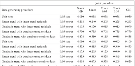
The literature contains several approaches to jointp-value computation, but it does not tell us which is best. To see whether my results are robust to different methods, I try four. Each involves a comparison of how unusual the actual boot-strappedp-values for the tests of interest are compared with the joint distribution of their simulated p-values for a given DGP. For a given set of tests, the joint distribution ofp-values reflects the correlations among the test statistics. I briefly describe the four joint methods here. Details are given in Appendix 2.

The first method is a bootstrapped version of the “improved Bonferroni procedure” of R. J. Simes (1986), which gives a jointp-value based on the actual

19. Of course, even my list of 42 tests omits many possible tests. There are other lag specification methods and an endless array of possible trend specifications, and no doubt additional unit root test approaches yet to be invented. I am implicitly assuming that as these possibilities increase in number, they become increasingly redundant and not remarkably more powerful.

p-values adjusted according to their number and rank in terms of size. The next two methods compute how unusual, relative to the bootstrapped distribution, are the actual number of individual rejections, i.e., the number of small-enough p -values (Cushman 2008). The two methods are differentiated by their use of the 0.05 or 0.10 level to determine rejection. The fourth method determines how unusual relative to the bootstrapped distribution are the specificp-values themselves (Cush-man and Michael 2011). There are several other techniques that I do not use (Ayat and Burridge 2000; Harvey et al. 2009; Hanck 2012) because they only apply to two tests.

I should provide evidence that the joint procedures I employ do work, in the sense of having good size and power properties. Existing evidence on the joint procedure properties is meager. Simes (1986) shows that his improved Bonferroni procedure has good size properties and better power than the standard Bonferroni method in the case of 10 tests, particularly when the test statistics are correlated. There is not any evidence concerning the counting methods I used in Cushman (2008). Nils Michael and I (2011) found good size properties for our approach as applied to six tests, but we did not examine power.

Given this shortage of evidence and the centrality of the joint approaches to my critique, I conducted a Monte Carlo examination of size and power of the unbootstrapped and bootstrapped Simes procedure, the 0.10 and 0.05 counting methods, and the Cushman-Michael procedure. The details are in Appendix 3. All the approaches have good size and power. The unbootstrapped and bootstrapped Simes p-values are very highly correlated (r ≥ 0.990) for every data-generating process, and so including just one is reasonable.

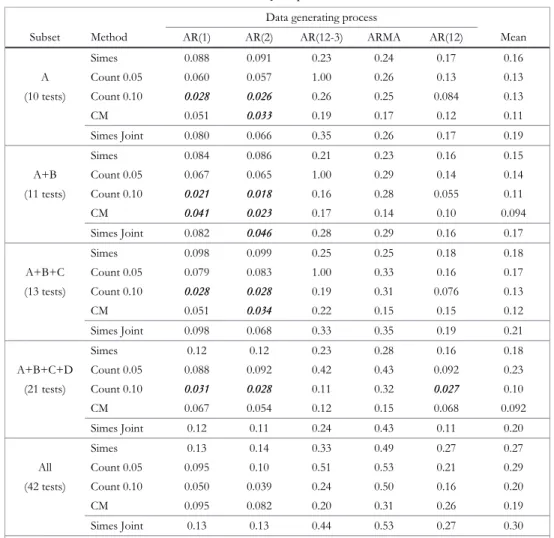
Table 3 gives the results for the four joint procedures for the various subsets of tests using the various DGPs. If one includes all 42 tests and uses the 0.05 level for rejection, the unit root is not rejected for any combination of DGP and joint p-value approach. But what if the significance level is relaxed to 0.10 or certain smaller test groups are considered more appropriate? Then unit root rejection remains possible. It depends on how we resolve the varying conclusions from the joint approaches, and on which DGPs are more plausible.

Let us first consider the issue of varying joint p-value conclusions. We are back to a multiple test problem. Given my conclusion that the four joint ap-proaches are all reasonable, then a joint approach can be applied to the joint tests. I therefore apply the unbootstrapped Simes procedure to the joint tests.20 _The

resultingp-values are labeled “Simes Joint” in Table 3. Only one is significant at the

0.05 level, for the subset A+B using the AR(2) DGP. However, several more are significant at the 0.10 level, for subsets A and A+B using the AR(1) or AR(2) DGP.

TABLE 3. Jointpp-values Data generating process

Subset Method AR(1) AR(2) AR(12-3) ARMA AR(12) Mean

Simes 0.088 0.091 0.23 0.24 0.17 0.16

A Count 0.05 0.060 0.057 1.00 0.26 0.13 0.13

(10 tests) Count 0.10 0.0280.028 0.0260.026 0.26 0.25 0.084 0.13

CM 0.051 0.0330.033 0.19 0.17 0.12 0.11

Simes Joint 0.080 0.066 0.35 0.26 0.17 0.19

Simes 0.084 0.086 0.21 0.23 0.16 0.15

A+B Count 0.05 0.067 0.065 1.00 0.29 0.14 0.14

(11 tests) Count 0.10 0.0210.021 0.0180.018 0.16 0.28 0.055 0.11 CM 0.0410.041 0.0230.023 0.17 0.14 0.10 0.094

Simes Joint 0.082 0.0460.046 0.28 0.29 0.16 0.17

Simes 0.098 0.099 0.25 0.25 0.18 0.18

A+B+C Count 0.05 0.079 0.083 1.00 0.33 0.16 0.17

(13 tests) Count 0.10 0.0280.028 0.0280.028 0.19 0.31 0.076 0.13

CM 0.051 0.0340.034 0.22 0.15 0.15 0.12

Simes Joint 0.098 0.068 0.33 0.35 0.19 0.21

Simes 0.12 0.12 0.23 0.28 0.16 0.18

A+B+C+D Count 0.05 0.088 0.092 0.42 0.43 0.092 0.23

(21 tests) Count 0.10 0.0310.031 0.0280.028 0.11 0.32 0.0270.027 0.10

CM 0.067 0.054 0.12 0.15 0.068 0.092

Simes Joint 0.12 0.11 0.24 0.43 0.11 0.20

Simes 0.13 0.14 0.33 0.49 0.27 0.27

All Count 0.05 0.095 0.10 0.51 0.53 0.21 0.29

(42 tests) Count 0.10 0.050 0.039 0.24 0.50 0.16 0.20

CM 0.095 0.082 0.20 0.31 0.26 0.19

Simes Joint 0.13 0.13 0.44 0.53 0.27 0.30

Notes: Ap-value of 1.00 means there were no rejections at the 0.05 level for the Count 0.05 test. In such cases I omit the test in computing the averagep-value. CM is the method of Cushman and Michael (2011).P-value significance is highlighted as in Table 2.

This brings us to the question of resolving the different results from different DGPs. We could assume that each is equally plausible. If so, multiplying each joint p-value by 1/5 and summing (i.e., computing the mean) generates an overallp-value for a given test group.21_{The final column of Table 3 gives the results. There are no}

rejections at the 0.05 level, but there are two marginal rejections at the 0.10 level.

21. This reflects the Law of Total Probability. Each individualp-value is the probability of a test statistic at least as extreme as the one observed given the DGP. Thus, the overall probability of a test statistic at least

But are the DGPs equally plausible? The data can be used to generate AIC and BIC weights using methods from Bruce Hansen (2007). Using AIC weights overwhelmingly favors the AR(12-3) model with a weight of 0.997. Using BIC weights almost equally favors the AR(12-3) model, with a weight of 0.932; the AR(1) is second at 0.067. With either the AIC or BIC, the weighted-meanp-values are essentially thep-values for the AR(12-3), and there are no rejections at even the 0.10 level.

The economic importance

of the permanent shocks

Given the failure to reject the unit root, from here on I assume real GDP has a unit root. I now present several estimates of the unit root’s economic impor-tance—addressing Ziliak and McCloskey’s (2008) desire for “oomph” analysis.

An unobserved components model

The first oomph estimate is from an unobserved components model. Krane (2011) also used such a model. The model gives an estimate of the relative magnitude of permanent shock variance to transitory shock variance. I use the local level model with constant drift in Koopman et al. (2000) and found in their STAMP software (version 6.21), which I use for the estimations. Letybe real GDP. The model is (with variables in logs):

(1a)

y_t=μ_t+ε_t , ε~NID

(

)

(1b)

μt=d+μt−1+ηt, η~NID

(

)

where ε is the transitory shock and η the permanent shock. The current, long-run level of yis determined byμt, and the long-run rate of growth is d. The key

parameters are the transitory varianceσ_ε2and permanent varianceσ_η2. To identify the two variances, Koopman et al. (2000) assume zero contemporaneous correlation between the errors. Serial correlation can be specified with the substitution of y_t− ∑_jk₌₁ρ_jy_t−jforytin equations (1a) and (1b). I use lag orderk= 3, consistent with

two lags in first differences as is sometimes suggested by the information criteria applied to the unit root tests. The substitution is equivalent to assuming thateandη are autoregressively correlated with identical lag coefficients.

An estimate of the relative importance of the permanent shocks is sη/se,

permanent to transitory shock standard deviation. The value for the 1947–2007 data is 1.17. This magnitude is, however, quite misleading because of significant small-sample bias. The estimation procedure has a hard time distinguishing partial persistence (ρj) from permanent persistence (η), and it tends to interpret partial

persistence as permanent. To compensate, I have computed bias-adjusted estimates. Details are given in Appendix 4. The mean-bias-adjusted ratio is 0.42. However, the estimate is subject to very large uncertainty (see Appendix 4).

Evidence from a vector error correction model

Cochrane (1994) proposed a two-variable vector error correction model (VECM) to identify the permanent and transitory components of real GDP. Non-durable goods consumption plus services consumption gives households’ perma-nent consumption. According to the permaperma-nent income hypothesis, permaperma-nent consumption is a random walk and is a constant fraction of permanent income on average. Thus, income (real GDP) and permanent consumption are cointegrated. Changes in permanent consumption reflect consumers’ views of permanent shocks to GDP. Deviations of GDP from the cointegration vector reflect transitory shocks to GDP. With two first-difference lags as employed by Cochrane (1994), the VECM model is:

(2a) ∆ct=ac+ec

(

)

(

)

(2b) ∆yt=ay+ey

(

)

(

)

wherecis permanent consumption andyis real GDP. With permanent consump-tion a random walk, ec = 0. The constant ratio of permanent consumption to

income gives the unitary coefficient onyt−1in the cointegration vector.22Actually, consumption in equation (2a) is not a pure random walk because of the presence of the first-difference lag terms. Nevertheless, theec= 0 constraint ensures that the

permanent shocks can be solely associated with consumption.23

22. The value of the ratio is contained in the constant of equation (2b), which also includes the long-run growth rate.

23. The constraint is accepted at the 0.05 level when the VECM is estimated over the 1947–2007 period and for three subperiods defined by consumption break dates of 1969:4 and 1991:4 found by Stock and Watson (2002).

I use the Cochrane VECM model to estimate the relative importance of permanent shocks. But what about possible structural change? Perron (1989) and Perron and Tatsuma Wada (2009) argued that a permanent change in real GDP’s growth rate occurred in 1973. Stock and Watson (2002) found a break in services consumption in 1969 and in nondurables consumption in 1991. There is also the Great Moderation (Kim and Nelson 1999). A VECM that is estimated for the entire data period but ignores such changes might give misleading results. Unfortunately, the dates are not definite and standard VAR/VECM estimation procedures do not allow for variance breaks. Therefore, I employ an alternative method, which is to estimate rolling VECMs. This approach gets estimates that gradually adapt to changing conditions. The rolling estimation periods are 15 years long.24

I use impulse response (IR) analysis to measure the importance of the unit root. Suppose some unexpected event, a shock, occurs. An impulse response is the deviation of a variable’s subsequent path from the path it would have followed if no shock had occurred. I wish to compare the effects of permanent shocks with those of transitory shocks. To do so unambiguously, we need a structural model with orthogonal permanent and transitory shocks. But the VECM is a reduced form model and does not reveal the orthogonal shocks. (The structural vector autoregression model can have unlagged terms forcandyon the right-hand sides of the equations.) To identify the structural model and shocks, I use the Choleski recursive approach. I assume that shocks to ycontemporaneously affect onlyy, notc, while shocks toccontemporaneously affect bothcandy. This follows from the permanent income model’s implication that consumption alone contains the single unit root process. If we were to reverse the Choleski ordering, orthogonal income shocks would have permanent effects, contradicting the model. Under the Choleski ordering I use, permanent shocks in the structural model are theυcterms

in the VECM consumption equation (2a).25_{The impulse responses are estimated}

with JMulti 4.24.

In the IR analysis, the magnitudes of the initiating shocks are the estimated standard deviations of the structural shocks over the estimation period (they are thus of ‘typical’ size). Withηthe permanent shock andethe transitory shock in the structural model, the initiating shocks for the impulse responses are thereforesηand

se. Across all 181 rolling models,sηhas a mean of 0.0041 andsehas a mean of 0.0067.

There is noticeable variation in both, illustrated below. The relative importance of the permanent shock,sη/se, has a mean across the 181 rolling periods of 0.64 (much

more than the estimate of 0.42 from the unobserved components model applied to the full data period).26

Important though the structural shock magnitudes are, IR analysis shows that their relative magnitudes are not very good indicators of subsequent real GDP responses. In what follows, the impact quarter is 0, and the forecast horizons are from 1 to 20 quarters ahead. To indicate relative importance, I report the sizes of the real GDP responses relative to the size of the initial transitory shock. In Figures 1a–1f, solid red solid lines depict permanent shocks or their GDP responses, and blue dashed lines depict transitory shocks or their GDP responses. The horizontal lines give the means across the 181 rolling periods. The dates on the horizontal axes give the starting period of the rolling VECM.

Figure 1a gives the actual shocks. A decline in shock magnitude in the Great Moderation is easily seen. Figures 1b–1f give GDP responses. At horizon 0 (the impact period), the response to the permanent shock averages half the value of the transitory shock. At horizon 1, the response to the smaller permanent shock has already caught up to that from the transitory shock. At horizon 4, the response to the permanent shock is on average 1.7 times the response to the transitory shock and 2.25 times the size of its initiating permanent shock. And at horizon 8, the permanent shock response is over 3 times the response to the transitory shock, and still 2 times the size of its initiating shock. During the Great Moderation, the responses at horizons 4 and 8 to transitory shocks have become relatively more important, but still not equal to those from permanent shocks. Note also that, at longer horizons, the growing relative importance of the permanent shock is increasingly a consequence of the dying away of the effects of the transitory shock.

25. If we don’t impose the permanent income model, then we can relax its error correction zero restriction on consumption adjustment and try both Choleski variable orderings. As a check, I compared the results of these alternative specifications with those of my main model using the full 1947:1 to 2007:3 period. The only significant difference is that, with income first in the ordering, it takes two years instead of less than one for consumption shocks to dominate income shocks in their effects on real GDP. The responses to income shocks continue to largely die away, just taking a bit longer.

26. Note that 0.64 ≠ 0.0041/0.0067: the mean of the ratios is not equal to the ratio of the means.

Figure 1a. Initial shocks (horizon 0) Figure 1b. Impulse responses at horizon 0

Figure 1c. Impulse responses at horizon 1 Figure 1d. Impulse responses at horizon 4

Figure 1e. Impulse responses at horizon 8 Figure 1f. Impulse responses at horizon 20

By horizon 20, the responses are close to their long-run values, with the permanent shock response 1.5 times its initiating shock in all but the early rolling VECMs, and the transitory shock response nearly back to zero. From these results, it would be hard to argue that permanent shocks are unimportant.27

These results are similar to those of Cochrane (1994). For instance, the mag-nitudes of the absolute and relative sizes of shocks and their responses at horizons 0, 4, and 8 are almost the same. Differences likely reflect that Cochrane (1994) did not imposeec= 0 when computing impulse responses, and that he did not compute

rolling VECMs. Because he did not imposeec= 0, a small part of Cochrane’s GDP

shock is permanent and never dies away. The rolling approach then reveals that transitory shocks become relatively more persistent during the Great Moderation (GDP’s relative responses to transitory shocks become larger at horizons 4 and 8).

Forecasting contests

The measures of unit root oomph presented so far are computed from within-sample data. Let’s turn to out-of-sample forecasts. I compare the forecasts of 6 models. The first two are the just-analyzed bivariate VECM and a univariate ARMA(2,2) in first differences. These specify both permanent and temporary shocks.28_{They are therefore unit root models. The second two models are a}

uni-variate AR(2) in first differences and a biuni-variate VAR(2) in first differences using real GDP and permanent consumption. These two models (called AR-dif and VAR-dif below) specify all shocks as having permanent effects, although they do allow transitory dynamics. These, too, are unit root models. The final two models are a univariate trend stationary AR(3) model in levels and a bivariate trend stationary VAR(3) model in levels (with real GDP and permanent consumption). In these two models (called AR-tr and VAR-tr below), all shocks are transitory.

The first forecasting experiment applies the rolling regression approach to the six forecasting models to make forecasts at horizons ofh= 1 to 20. The number ofh-period-ahead forecasts for each model and horizon is 181 −h. My measure of forecast accuracy is the square root of the mean squared forecast error, i.e., the standard deviation of the forecast errors where the mean in the standard deviation formula is set to zero.29_{Results for a few key horizons are in Figures 2a and 2b.}

Each cluster of bars shows the forecast error standard deviations for the six models for one forecast horizon. The vertical axis measures the values of the forecast standard deviations. Figure 2a is computed using all forecasts through 2007:3.

Fig-28. I have already discussed the way the VECM specifies permanent and transitory shocks. Tsay (2005) shows how various ARMA models are reduced forms of unobserved component models with permanent and transitory shocks.

29. Mean square forecast errors, not standard deviations as I am using, are often employed to reflect the assumption that large errors are disproportionately more costly than small errors. And they assume the disproportionalities are specifically quadratic. The reader can make adjustments if desired. I employ standard deviations so that the differences among them correspond to easy-to-interpret growth rates, not squared growth rates.

Figure 2a. Forecast error standard deviations: earliest through 2007:3

Figure 2b. Forecast error standard deviations: 2007:4–2013:4

ure 2b shows forecasts from 2007:4 through 2013:4 (for the first time in the paper). The longer-horizon forecasts are dominated by the inability to forecast the Great Recession.

In Figure 2a, the unit root models almost always outperform the linear trend stationary models (in 27 of 32 paired comparisons—four unit root models with two trend stationary models for four horizons). The VECM model always is best. But the margins of victory for the unit root models are not usually large in relative terms. The unit root models win less often in Figure 2b (23 of 32 comparisons), but the VECM model is still best in every case.30

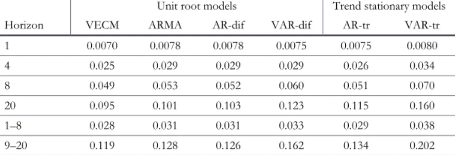
Tables 4a and 4b give the underlying numerical values for Figures 2a and 2b, with the addition of summary measures in the form of the mean forecast standard errors for horizons 1–8 and 9–20. The previous conclusions are supported, with the additional revelation that, for the means, every unit root model beats the trend stationary models for forecasts through 2007:3.

Interest in unit root models and forecasting has often centered on whether or not recoveries from recessions would be robust, involving rebounds. Thus, for the second forecasting contest I use actual postwar recessions. Suppose, in what turns out to be the final quarter of the seven postwar recessions with sufficient data preceding them, a hypothetical econometrician uses the above six models to forecast the recovery. The models are estimated using the 60 quarters of data ending in the last quarter prior to the peak that defines the beginning of recession

according to the BEA. This is to follow a number of economists who, as previously mentioned, implicitly or explicitly drew trend lines based on pre-recession data.31

TABLE 4a. Forecast standard errors, from first rolling model through 2007:3

Unit root models Trend stationary models

Horizon VECM ARMA AR-dif VAR-dif AR-tr VAR-tr

1 0.0072 0.0084 0.0080 0.0075 0.0083 0.0081

4 0.019 0.023 0.022 0.020 0.024 0.026

8 0.031 0.036 0.035 0.033 0.039 0.043

20 0.0501 0.052 0.052 0.052 0.0503 0.054

1–8 0.020 0.023 0.023 0.021 0.025 0.027

9–20 0.043 0.0466 0.0457 0.045 0.0468 0.052

TABLE 4b. Forecast standard errors, 2007:3–2013:4

Unit root models Trend stationary models

Horizon VECM ARMA AR-dif VAR-dif AR-tr VAR-tr

1 0.0070 0.0078 0.0078 0.0075 0.0075 0.0080

4 0.025 0.029 0.029 0.029 0.026 0.034

8 0.049 0.053 0.052 0.060 0.051 0.070

20 0.095 0.101 0.103 0.123 0.115 0.160

1–8 0.028 0.031 0.031 0.033 0.029 0.038

9–20 0.119 0.128 0.126 0.162 0.134 0.202

Note: I sometimes increase decimal accuracy beyond three places to allow distinction of slight differences in magnitude, but this is not to imply that such differences are necessarily of statistical or economic significance.

The results are presented graphically in Figures 3a–3g. The figures include 20 forecast periods after the end of the recession and six quarters prior. In two cases, the 1969:4–1970:4 and 1980:1–1980:3 recessions, the next recession starts before 20 quarters have elapsed. In these cases, vertical lines indicate the middle of the peak quarter that defines the beginning of the next recession. All values are detrended with a simple OLS linear trend from the same 60-quarter forecast period used for the forecasting models. The horizontal zero line corresponds to this trend.

31. My results will not be precisely what the hypothetical econometrician would have obtained in real time because I am using 2014 vintage data, not the data available at the time of the forecasts. In addition, several of the modeling techniques had not been invented at the time of the earlier recessions. Finally, since real-time econometricians would not know the ending period of the recession until sometime later, my approach gives the trend stationary models an advantage in that, if there is going to be a return to a former trend line, it should be most accurately measured starting at the end of the recession.

Fig. 3a. After the 1969:4–1970:4 recession Fig. 3b. After the 1973:4–1975:1 recession

Fig. 3c. After the 1980:1–1980:3 recession Fig. 3d. After the 1981:3–1982:4 recession

Fig. 3e. After the 1990:3–1991:1 recession Fig. 3f. After the 2001:1–2001:4 recession

After recessions 1 (1969:4–1970:4), 3 (1980:1–1980:3), and 4 (1981:3– 1982:4), real GDP more or less returns to the simple prior trend given by the zero line. However, in contrast to some beliefs previously noted, real GDPoften has no tendency to return to a prior trend; see recessions 2 (1973:4–1975:1), 5 (1990:3–1991:1), and 7 (2007:4–2009:2). And after recession 6 (2001:1–2001:4), GDP’s path follows an ambiguous path. It thus appears that the relative importance of the permanent and transitory shocks associated with recessions has varied.

Which forecasting models manage these diverse situations best? Consider the two linear trend stationary models (AR-tr and VAR-tr) versus the two first difference models (AR-dif and VAR-dif). The linear trend stationary models do better when GDP heads back to the prior trend. This is not surprising as these models always assume reversion to trend. The first difference models do better when there is no significant return to the former trend, again unsurprising as these models assume shocks are permanent. The first difference models somewhat out-perform the trend stationary models in the ambiguous case of recession 6. But what about the ARMA and VECM models? The graphs suggest that the ARMA model is a sort of compromise, consistent with its forecasts estimating any recent shock to be a typical blend of permanence and transience. The VECM provides a better compromise, doing reasonably well after every recession, which can be attributed to its explicit, and apparently often successful, identification of recent permanent versus transitory shocks. Thus, unless you know what kind of shock caused the recession, the VECM seems to be the best choice.32

The impressions from looking at Figure 3 are sharpened by examining the forecast error standard deviations. I compute them for the six models and seven recessions using the same 20 post-recession quarters as in Figure 3, except for the two recessions where another recession intervenes in less than 20 quarters. In those cases, the final forecast error quarter is that of the peak defining the beginning of the next recession. The results are in Figure 4.33_{For example, as it appeared from}

the graphs, after recessions 2, 5, 6, and 7, the trend stationary models generally do much worse than the models specifying unit roots. The trend stationary models do well after recessions 1, 3, and 4. The VECM model, although frequently not the best, always does fairly well with no huge mistakes as sometimes occur with the other models.

32. Regarding the VECM’s success in forecasting no recovery from the last recession, Cochrane (2015c) remarked: “It’s interesting that consumers seem to have seen the doldrums coming that all the professional forecasters did not.”

33. The forecast error bars from the linear trend stationary models for the final recession are so large that I have truncated the height of the graph to maintain reasonably visible differences among the other forecast error bars.

Figure 4. Forecast error standard deviations after recessions

I obtain overall conclusions from the Figure 4 results by computing averages of each model’s forecast error standard deviations across the recessions. They are in Table 5. The first row gives the arithmetic means of the seven forecast error standard deviations for each model. The second row gives the means with forecast error standard deviations weighted by the number of forecast periods used to compute them (fewer for the two recessions whose recoveries were cut short by another recession). The mean standard deviations for the AR-tr and VAR-tr models are strongly influenced by very large forecast error standard deviations for the final recession. To see what difference the last recession makes, the third and fourth rows omit the last recession.

TABLE 5. Average forecast error standard deviations across recessions

Unit root models Trend stationary models

Type of average VECM ARMA AR-dif VAR-dif AR-tr VAR-tr

Mean 0.014 0.020 0.025 0.026 0.028 0.044

Weighted mean 0.015 0.024 0.031 0.031 0.038 0.060

Mean

without last recession 0.014 0.021 0.028 0.029 0.020 0.026

Weighted mean

without last recession 0.016 0.027 0.036 0.036 0.027 0.036

models explicitly specifying only permanent shocks, AR-dif and VAR-dif, are next best. The linear trend models are worst. Accordingly, concluding that GDP is trend stationary, or that unit roots don’t matter, is likely to lead to the worst forecasts, on average. Meanwhile, if the 2007:4–2009:2 recession is omitted, perhaps because one believes it was an extraordinary event, the tidy pattern just described is somewhat muted. In rows 3 and 4, the ARMA is now only the approximate equal of the AR-tr. The VECM model, however, continues to be substantially better than the other models.

The above results suggest that:

1. Models specifying only one kind of shock only do well when that kind of shock dominates. The modest advantage on average of the AR-dif and VAR-dif models over the AR-tr and VAR-tr models thus reflects a history where the causes of recessions have been dominated by permanent shocks a bit more often than by transitory shocks. 2. The ARMA and VECM outperform the other models because they

allow both kinds of shocks. However, the multivariate approach of the VECM is significantly better than the ARMA approach because, unlike the univariate ARMA model, a multivariate approach has the potential to separately identify the two kinds of shocks.

3. The advantage of a multivariate model disappears entirely if it is misspecified as trend stationary. In the tables, the VAR-tr model is generally the worst of all.

Final remarks

I have first provided evidence that, despite a significant literature to the contrary, the null hypothesis of a unit root in U.S. real GDP in postwar real GDP cannot be rejected. The key innovation is to account for the multiple test problem. Nevertheless, failure to reject is not a strong result, and it may well be that lack of power still hobbles the unit root testing approach despite all the data now available. It is also surprising that a large literature testing the trend stationarity null did not arise, although those tests may also lack sufficient power. Regardless, the difficulty of discerning between nearly equivalent null and alternative hypotheses in the unit root context has long been understood (see discussion by Stock 1990).