Contents lists available atSciVerse ScienceDirect
Future Generation Computer Systems
journal homepage:www.elsevier.com/locate/fgcs
Enabling cost-aware and adaptive elasticity of multi-tier cloud applications
Rui Han
,
Moustafa M. Ghanem
,
Li Guo
,
Yike Guo
∗,
Michelle Osmond
Department of Computing, Imperial College London, London SW7 2AZ, UK
a r t i c l e i n f o
Article history:
Received 30 October 2011 Received in revised form 30 March 2012 Accepted 17 May 2012 Available online xxxx Keywords: Cloud computing Elasticity Multi-tier applications Cost-aware criteria Adaptive scaling algorithm
a b s t r a c t
Elasticity (on-demand scaling) of applications is one of the most important features of cloud computing. This elasticity is the ability to adaptively scale resources up and down in order to meet varying application demands. To date, most existing scaling techniques can maintain applications’ Quality of Service (QoS) but do not adequately address issues relating to minimizing the costs of using the service. In this paper, we propose an elastic scaling approach that makes use of cost-aware criteria to detect and analyse the bottlenecks within multi-tier cloud-based applications. We present an adaptive scaling algorithm that reduces the costs incurred by users of cloud infrastructure services, allowing them to scale their applications only at bottleneck tiers, and present the design of an intelligent platform that automates the scaling process. Our approach is generic for a wide class of multi-tier applications, and we demonstrate its effectiveness against other approaches by studying the behaviour of an example e-commerce application using a standard workload benchmark.
©2012 Elsevier B.V. All rights reserved.
1. Introduction
Cloud computing has received wide attention over the past few years. New services offered by cloud IaaS (Infrastructure-as-a-Service) providers, such as Amazon Web Services (WS) [1], GoGrid [2] and IBM [3], are generating a huge demand from ap-plication owners. The pay-as-you go model used by such providers is appealing to most application owners. It removes the costs of buying, installing and maintaining a dedicated infrastructure for running an application. Moreover, most IaaS providers allow the application owners to scale up and down the resources used based on the computational demands of their applications, thus letting them pay only for the amount of resources they use. This model is appealing for deploying applications that provide services for third parties, e.g. traditional e-commerce sites, financial services appli-cations, online healthcare appliappli-cations, gaming appliappli-cations, me-dia servers and bioinformatics applications. If the workload of a service increases (e.g. more end users start submitting requests at the same time), the application owner can ideally scale up the re-sources used to maintain the Quality of Service (QoS) of their ser-vice. When the workload eases down, they can then scale down the resources used. Within this context, elasticity (on-demand scal-ing), also known as redeploying or dynamic provisioning, of ap-plications has become one of the most important features of a
∗Corresponding author. Tel.: +44 07869562039.
E-mail addresses:[email protected](R. Han),[email protected]
(M.M. Ghanem),[email protected](L. Guo),[email protected](Y. Guo),
[email protected](M. Osmond).
cloud computing platform. This elasticity enables real-time ac-quisition/release of computing resources to scale the applications themselves up and down in order to meet their run-time require-ments, while letting application owners pay only for the resources used.
Our motivation in this paper is investigating the development of new methods that assist the owners of applications deployed on IaaS clouds in managing the costs of their own applications while still maintaining the Quality of Service (QoS) they provide to their end users. Addressing this issue effectively requires taking a closer look at the structure of most common services and applications deployed on IaaS clouds to provide services to other parties. Such applications are typically implemented as multi-tier applications running on distributed software platforms. Taking the example of an e-commerce website, there are at least three tiers: a frontend web server for handling HTTP requests; a middle-tier application server for implementing business logic; and a backend database with data store and processing. Each of the tiers can be implemented using one or more servers. Depending on different types of incoming requests, servers at each tier can be stressed by heavy workloads, or can become idle due to light workloads. When scaling up and down an application, it is thus crucial to discover the real bottlenecks that may be caused at any, or all, of the servers.
Although some of the existing scaling techniques [1,4–16] address the question of how to maintain an applications’ Quality of Service (QoS), they rarely consider the equally important aspect of cloud computing—the cost of using the resources themselves. Applications deployed in a cloud environment require both good performance and cost-efficient resource usage.
In this paper, we propose a scaling approach that is both cost-aware and workload-adaptive, allowing application owners to
0167-739X/$ – see front matter©2012 Elsevier B.V. All rights reserved.
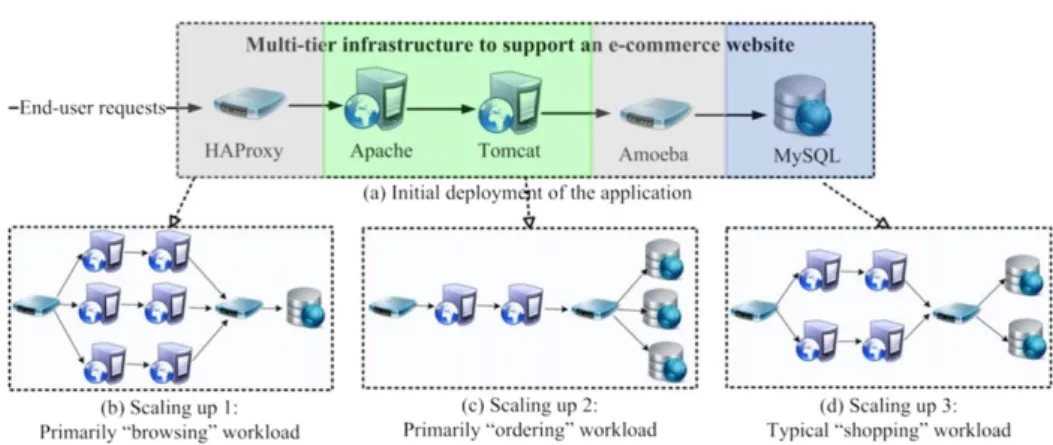
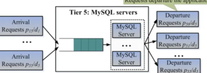
Fig. 1. Multi-tier infrastructure of an e-commerce website and three types of workloads.
perform more efficient cloud elasticity management. The paper features four key elements:
•
Cost-aware criteria: a flexible analytical model is developed to capture the behaviour of multi-tier applications. Cost-aware criteria are introduced to measure the effect of cost of resources on every unit of response time.•
Workload-adaptive scaling: using the above criteria, a Cost-Aware Scaling (CAS) algorithm is designed to handle changing workloads of multi-tier applications by adaptively scaling up and down bottlenecked tiers within applications.•
Automation of application scaling: a standard and extensible specification is introduced to describe the properties of the servers, including their VM configuration, IaaS user settings, linking relationships and other constraints. Based on this specification, the best cost-aware scaling approach required for an application can be automatically computed and executed.•
Implementation and experimental evaluation: an intelligent platform based on the CAS algorithm is implemented to automate the scaling process of cloud applications on the IC-Cloud infrastructure [17]. The proposed cost-aware ap-proach is tested using an industry standard benchmark [18] and the test results show: (1) the CAS algorithm responds to chang-ing workloads effectively by scalchang-ing applications up and down appropriately to meet their QoS requirements; (2) deployment costs are reduced compared to other scaling techniques. The remainder of this paper is organised as follows: Section2 il-lustrates the need for this new approach to elasticity by describing some current examples and challenges; Section3discusses related work; Section4provides a more detailed overview of the proper-ties of typical multi-tier applications and describes the architecture of the Imperial Smart Scaling engine (iSSe) implemented to support our approach; Section5explains the proposed CAS algorithm and its details; Section6reports the experimental evaluation of the al-gorithm’s effectiveness; Sections7and8present discussion of the approach and summarise directions for future work.2. Motivation
This section illustrates two challenges that need to be addressed in order to achieve elastic scaling in a large class of multi-tier applications deployed on IaaS clouds. Without loss of generality, we use a simple example based on an e-commerce website to capture the typical behaviour of such applications. Also for simplicity, we focus only on applications that are deployed on the resources of single IaaS cloud provider. As discussed in the introduction, the workload for such applications depends on the number of end users submitting requests at the same time. The workload may be composed of different types of requests that need to be handled by different parts of the application. For example
some end users may be browsing the web site itself, while others may be querying the product catalogue or making a payment transaction. To highlight the key challenges, consider the typical infrastructure for a multi-tier e-commerce application as shown in
Fig. 1(a). This application is composed of five tiers of components (servers): the HAProxy and Amoeba load-balancing servers, the Apache HTTP server, the Tomcat application server and the MySQL database server. These servers work together to handle end users’ requests. Depending on the application workload, servers at each tier can be stressed at different times and the application owner would need to scale up or down the appropriate resources to maintain the QoS of their application.
Challenge1:Cost-aware scaling. In a highly scalable cloud en-vironment where computing resources are consumed as a utility such as water and electricity [19], application owners would ex-pect to spend the least cost for the desired application perfor-mance. To this aim, the elastic scaling must take cost-aware criteria into consideration and use them to guide application scaling. Take
Fig. 1(a)’s application for example, these criteria should be aware of both the cost of adding a server (e.g., an Apache or a MySQL) and the performance effect brought by this scaling up (e.g., reducing response time).
When the application is initially deployed (Fig. 1(a)), five servers of this application are hosted across different VMs to support a small number of customers. When the demand increases, the application should be scaled up. An interesting point here is that this scaling process is greatly influenced by the behaviour (i.e., the type of workload) of the application itself. We examine three typical types of workloads, where each workload places varying demands on different tiers of the application. In the primarily ‘‘browsing’’ workload (Fig. 1(b)), end users mainly browse webpages and preview products. This workload mainly stresses the service tier including the Apache and Tomcat servers, so their resources are saturated and the number of these servers needs to be increased. By contrast, the primarily ‘‘ordering’’ workload mainly stresses the storage tier including the MySQL database and so the number of these database servers needs increasing (Fig. 1(c)). Finally, the typical ‘‘shopping’’ workload simultaneously stresses the service and storage tiers and so the number of servers in both two tiers is increased (Fig. 1(d)).
Challenge 2: Workload-adaptive scaling. Due to the dynamic cloud environment, two types of uncertainties exist in the application workload: (1) the type of workload, such asFig. 1’s three types of workload; (2) the volume of workload, which is denoted in terms of the arrival rate of incoming requests, namely the number of incoming requests per time unit. In this context, the elastic scaling must be adaptive to the changing workload, and such adaptive scaling has triple meanings. First of all, bottleneck tiers of applications should be automatically identified both for scaling up and down. Secondly, scaling should be performed as
an iterative process because fixing a bottleneck tier may create another bottleneck at a different tier of the application. For instance, inFig. 1(d)’s workload, the bottleneck is shifted to the storage tier if multiple Apache and Tomcat servers are added to the service tier. Finally, agile scaling is needed to rapidly restore acceptable application performance.
In the remainder of this paper we develop a framework and algorithms that address both challenges effectively. We implement and evaluate our approach using the IC-Cloud platform [17] as an example. The advantage of using the IC-Cloud platform is that supports a fine-grained pricing strategy (e.g., VM instances are charged by minute rather than by the hour as in Amazon WS) which simplifies the evaluation. However, the approach and algorithms are generic and can be applied on most IaaS environments.
3. Related work
3.1. Traditional scaling techniques before clouds
Scaling of applications has been studied extensively before clouds. Early work considers single-tier applications and focuses on transforming performance targets into underlying computing resources such as CPU and memory [4–6]. Further investigations classify an application into multiple tiers [7–10]. They then break down the end-to-end response time by each tier and conduct the worst-case capacity estimation to ensure applications meeting the peak workload. Overall, the single-tier model can be viewed as a special case of a multi-tier model and the latter model can guide the scaling in a more accurate way.
However, although scaling of traditional applications, which are often hosted on physical servers, shares many commonalities with that of cloud applications, these two types of scaling technique have different emphases. Conventional techniques mainly concentrate on how to schedule compute nodes to meet the QoS requirements of applications by predicting their long-term demand changes. In contrast, clouds focus on providing metered resources on-demand and on quickly scaling applications up and down whenever application demand changes. Further investigations, therefore, are needed to address the challenges brought about by this requirement for high elasticity. For example, a CloudSim toolkit is proposed to simulate an application in order to accurately estimate its required resources before the actual deployment in clouds [20]. Another example, Merino et al. introduce a hybrid grid-cloud architecture and propose a market-based economic mechanism to assist grid users in performing scaling with cloud resources [21].
3.2. Policy-based scaling techniques
At present, numerous efforts have contributed to scale cloud applications. Some resource provisioning systems [22], frame-works [23,24] and lifecycle management toolkits [25] are proposed to manage cloud resources based on the idea of autonomic con-trol [26]. Rather than developing concrete scaling methods, these studies generally discuss higher-level concerns in building an ef-fective provisioning system. Examples are performance metrics used in resource allocation, service-level agreement (SLA) analyser, performance monitor and VM allocator.
Most of the cloud providers (e.g., Amazon WS [1]) and vendors (e.g., RightScale [11]) employ pre-defined policies (or rules) to guide application scaling. Taking RightScale [11] as an example, application owners need to manually define an application’s rules for triggering scaling after its deployment. These rules specify the minimum and maximum number of servers in the application, the condition to scale these servers, the number of servers in each scaling and even the scaling speed. Server monitor triggers
these rules to perform scaling. Inheriting from Rightscale, UniCloud extends the policy-based scaling by considering further issues such as work priority and CPU speed [12]. In addition, Nathania et al. introduce four types of policy to manage the allocation of VMs for different types of applications [13].
Policy-based scaling allocates additional servers in scaling up whenever some performance metrics exceed a threshold and removes redundant servers in scaling down whenever these metrics are less than a threshold. This scaling mechanism assumes that application owners have the relevant knowledge of the application being executed to define proper policies and this assumption is sometimes not applicable to application owners. In addition, this kind of scaling is designed to meet applications’ QoS requirements, and cost-effective resource provision is not achievable in many cases.
3.3. Scaling techniques using analytical models
Many researchers apply the analytical modelling technique to help application owners make scaling decisions by informing them of the performance analysis results of applications. Xiong et al. model an application by a network of queuing models and conduct the performance analysis to show relationships among workloads, server number and QoS level [27]. In [28], Ghosh et al. divide an application into three types of sub analytic model: the resource provisioning decision model, VM provisioning model and run-time model. By iteratively solving each individual sub-model, their analysis obtains two results: response time and service availability. In addition, Ghosh et al. utilise a stochastic reward net to model an application and give two analysis results: job rejection rate and response delay [29]. In [30], Pal et al. propose a pricing framework with economic models designed for multiple cloud providers in the marketplace, where each cloud provider is modelled as a queueing system. Using this queueing system, the framework aims at informing application owners of the price and its related QoS level. In [31], Huu et al. introduce several network provisioning strategies based on a cost estimation model. These strategies are used by application owners to predict the amount of resources and their deploying cost for an application.
Moreover, a variety of application scaling approaches are proposed using the analysis results of queueing models. In [14], Bacigalupo et al. model an application by a queueing model with three tiers, namely application, database and database disk tiers. Each tier is then solved to analyse the mean response time, throughput and utilisation of a server. Using these results, a resource management algorithm is proposed to scale applications in dynamic-urgent clouds.
Similar to [7–10], Bi et al. break down an application’s end-to-end response time to each tier [15]. They then calculate the number of servers allocated to the application subject to constraints of average response time and arrival rate.
In [16], Hu et al. consider two allocation strategies using queueing models: (1) shared allocation (SA) strategy where all incoming requests have the same queuing; (2) dedicated allocation (DA) strategy where requests with different arrival rate are divided into multiple queues. An algorithm is then proposed to decide which strategy (SA or DA) requires the smaller number of servers to satisfy the QoS requirement.
Other stochastic models are also applied in guiding the scaling of applications. In [32], Iqbala et al. present a methodology supporting both the scaling up and down of a two-tier web application. Scaling up is based on a reactive model that actively profiles CPU utilisations of VMs. Scaling down uses a regression-model-based predictive mechanism. In addition, Li et al. use a network flow model to analyse applications and introduce an approach to assist application owners in making a trade-off between cost and QoS [33].
To the best of our knowledge, previous scaling techniques either provide general information to application owners and rely on them to make proper scaling decisions [27–31], or propose scaling approaches using the analysis results of analytical models [7–10,14–16]. This sort of investigation has solved the scaling of applications to meet their QoS satisfactorily. However, existing scaling approaches rarely consider the equally important issue of cloud computing—the cost. Applications deployed in a highly scalable cloud environment require not just good performance but also cost-efficient resource provision. An elastic scaling approach for more efficient cloud elasticity management, therefore, could be a desirable advance.
4. A system to support elastic scaling
In this section, we first present an overview of the properties of multi-tier applications (Section4.1). A platform, called iSSe, is then introduced to support the elastic scaling of these applications (Section4.2). Finally, we explain how iSSe achieves the automation of application scaling (Section4.3).
4.1. Multi-tier cloud applications
A cloud application can either be an infrastructure application or an end-user application [34]. Examples of infrastructure appli-cations are DNS servers, email servers or databases. Appliappli-cations of this sort often have simple structures, such as having one or two tiers. By contrast, the structure of an end-user application is more complex. For example, the e-commerce website inFig. 1has five tiers. This work uses an end-user application as an example be-cause it can also incorporate the simpler infrastructure application scenario.
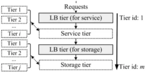
In a multi-tier application, servers are categorized into different tiers according to their functionalities, as listed inFig. 2: servers at the two load balancing (LB) tiers, such as HAProxy and Amoeba, distribute requests to servers at the service or storage tiers; servers at the service tier, such as Apache and Tomcat, are responsible for handling HTTP requests and implementing business logic; and servers at the storage tier, such as the MySQL database, are used for managing application data. In addition, servers at the service or storage tier can be further divided into different sub-tiers.
Typically, each application has a set of demands and constraints specified by the application owner in the form of a SLA. A performance demand is defined by the maximum end-to-end response time for a request. This time can either be an average response time or a high percentile of response time distribution (e.g., 90% of the response times should be less than 2 s). A cost constraint is the budget of the total application deployment. In addition, each tier has a resource constraint that restricts the maximum number of servers in this tier. For instance, the maximum number of Tomcat servers is 10.
Definition 1 (A Multi-tier Application). A multi-tier application consists of two parts: (1) the server setS, including all servers of the application, and (2) the demand setD, capturing the requirements specified in the SLA.
The multi-tier architecture guarantees the modularity of cloud applications and facilitates the control of their tiers. An application’s server set can be divided into multiple subsets and each subset consists of servers belonging to the same tier. Each server is marked by a unique tier id. For instance, inFig. 1, for an e-commerce website, the tier ids of HAProxy, Apache, Tomcat, Amoeba and MySQL are 1–5, respectively. Starting from HAProxy, which acts as the end users’ communication interface, servers at each tier first receive in-processing requests from the previous tier, process these requests locally and then transmit them to the next tier.
Fig. 2. The multi-tier architecture of cloud applications.
Fig. 3. The architecture of iSSe.
Definition 2(Server’s Tier Id).In am-tier application, each servers
has a unique tier ID, denoted byid
(
s)
. Servers’ tier ids are numbered consecutively from 1 tomaccording to these servers’ tier types: LB tier for Service, Service tier, LB tier for Storage and Storage tier.Definition 3(Server Subsets).In am-tier application, the server set
Scan be divided intomserver subsets:S1
∪
S2∪ · · · ∪
Sm, whichare sorted in strictly ascending order according to the tier id of their servers. That is, each subsetSi consists of servers belonging
to tieri
(
i=
1, . . . ,
m)
and for any pair of serverssands′, we haveid
(
s) <
id(
s′)
ifs∈
Siands′
∈
Si+j(
0<
j≤
m−
i)
.4.2. iSSe to support elastic scaling
As shown in Fig. 3, iSSe acts as middleware between cloud providers and application owners. TheIaaS User Portal of iSSeassists application owners to conveniently provide services to application end users. Using this portal, application owners can specify the required response time for their applications, select the needed servers and their configuration from theRepository of Servers, and get notified when workload violation happens and applications are scaled up (down).
In addition to the IaaS User portal, the other four service components in iSSe work together to support elastic scaling. The
Monitoring Servicemonitors each running application using two types of monitor (seeFig. 4). The first type of monitor is the
entry monitor, which examines the incoming requests over a finite interval (e.g., 60 s) and records information such as the request arrival rate. This information is used to decide whether a scaling up (or down) is needed. For instance, scaling up is triggered if the observed response time exceeds the response time threshold defined by the application owner. The second type of monitor is the
server monitorinstalled on each server. This monitor examines the server’s resource usage (e.g., CPU utilisation), analyses tier-specific values, such as response time, and collects other server execution logs. All monitoring information is stored in a database. When a scaling is triggered, the Capacity Estimation Service conducts a scaling algorithm (e.g., CAS algorithm explained in Section5) and estimates the number of servers to be scaled using the information in the database. Subsequently, theDeployment Service
Fig. 4. The monitoring service of iSSe.
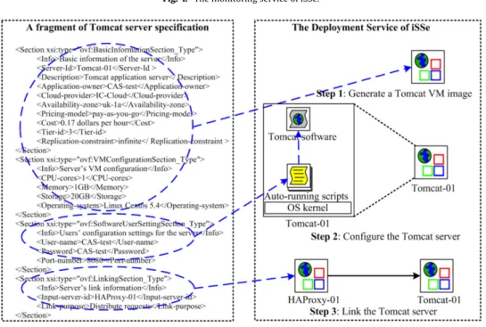
Fig. 5. The automatic addition of a Tomcat server in the Deployment Service.
automatically implements the scaling of these servers by calling interfaces in IC Cloud [17]. In the scaling process, all information related to the multi-tier configuration is obtained from servers’ specifications.
4.3. Server specification and automation of application scaling
In iSSe, each server is installed in a stand alone VM. As shown inFig. 4, this VM consists of installed software such as Tomcat software, as well as a server monitor and pre-loaded auto-running scripts used in automating the scaling process.
An XML-based specification is available to describe the key aspects of a single server by extending the Open Virtualization Format (OVF) open standard [34]. The OVF standard is widely adopted by key industry vendors, such as VMware, IBM and Oracle, to describe their VMs. Using this specification facilitates scaling in several ways: (1) different features of the server are described concisely and accurately; (2) automatic content validation and software licensing are supported based on an industry standard; (3) single server specifications can be saved as standard templates and a complex multi-tier application can be constructed by multiple interdependent templates; (4) the specification is independent of cloud vendor and platform.
Fig. 5 shows an example specification of the Tomcat server. This specification has four sections. The first section lists the
server’s basic information, such as its tier id and its replication constraints. The subsequent three sections define the server’s VM configuration, software user settings and links to other servers, respectively.
In theDeployment Service, the automatic scaling indicates that the scaling process, namelyaddition,removalandresource modifi-cationof servers, can be automatically executed by interpreting the servers’ specifications. Automating theadditionactivity involves three steps, as shown inFig. 5. In step 1, theDeployment Servicefirst generates a Tomcat VM image, as specified in theBasic Informa-tionsection andVM Configurationsection. In step 2, the VM is first started, after which the auto-running scripts preloaded in this VM use the parameters in theSoftware User Settingsection to configure the Tomcat software: the user name, password and port number of the Tomcat are set. At step 3, the Tomcat is linked to its input load-balancing server HAProxy-01, as specified in theLinkingsection.
The Addition operations take a few minutes to achieve. Typically, the generation of a VM image (step 1) can be finished within a few seconds. This is because after a server is packaged, most existing cloud platforms (including IC-Cloud and Amazon WS) usually keep a certain number of images ready for use. In addition, step 2 and 3 can be completed within 1 or 2 min. The time is mainly consumed in starting up the VM and executing the scripts to configure the server software. However, there are two situations when theadditionactivity may need a slightly longer
time to complete. The first situation is when a server at the storage tier is to be added. In this case, the server may need some time to update/replicate data. An example is when a newly added MySQL Slave needs to synchronize with the MySQL Master. The second situation arises due to the auto-running script of a LB server (e.g., a HAProxy), which executes once every few minutes. Hence when a new Service/Storage server (e.g., Tomcat) is added, it needs to wait until the LB server’s script runs again to detect and register this new server.
Automating theremovalactivity is achieved by conducting the reverse operations of the additionactivity: the running Tomcat server is disconnected from its input server HAProxy and removed from the application. Note that this server’s running VM instance is only shut down when its existing billing period ends. For example, most mainstream providers, such Amazon WS, today bill their users by the hour. However, the CAS algorithm can charge VM instances in a finer granularity than per hour in order to achieve cost-efficient scaling. For example, a server s1 is added to an application att
=
0 (time unit is minute), it is removed att=
5 and added att=
15; it is removed again att=
30 and added back to the application att=
45. Assuming that servers1is charged by minute in the CAS framework, its cost is less than a servers2that keeps running for an hour:c(
s1)=
(
35/
60)
c(
s2)because servers1only runs, and is charged for, 35 min. This fine-grained pricing strategy is supported in the IC-Cloud platform (e.g., a VM instance is billed by the minute).
Theresource modificationactivity is conducted if information in the Tomcat’s specification is updated. This activity reconfigures the VM, resets the Tomcat’s user settings and links to related servers. The reconfiguration of the VM is based on the observation that multiple basic (smallest) resource units can constitute a VM and so the VM configuration can be modified by changing the number of these units. For instance, one basic resource unit can be equivalent to one VM with one 40 GHz CPU, 1 GB memory and 10 GB storage. If each server is hosted in a VM with one basic resource unit, increasing or decreasing a unit in theresource modificationactivity could have equivalent effect to additionorremoval of a server. The fine-grain management of the VM and fine grained resource-level scaling are discussed in our complementary work [35], which models each basic resource unit by a vector consisting of multiple dimensions, including CPU, size of memory, I/O amount, allowing both the performance and cost of individual units to be analysed precisely.
5. The CAS algorithm
In this section, we provide an overview of the CAS algorithm (Section5.1) and introduce two cost-aware criteria to guide scaling up and down of applications (Section5.2). Using these criteria, we then present two capacity estimation algorithms: the Cost-Aware-Capacity-Estimation (CACE)-For-Scaling-Up (Section 5.3) and CACE-For-Scaling-Down (Section 5.4). We also define the performance metrics to evaluate the behaviour of the scaled applications (Section5.5).
5.1. The algorithm overview
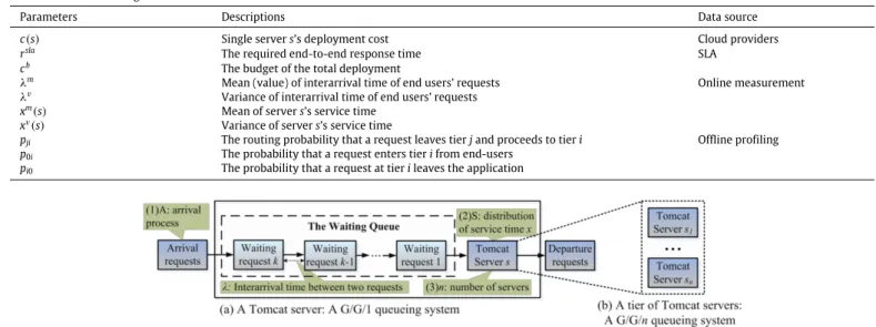
For clarity, Table 1 lists the main parameters of a m-tier application used throughout the CAS algorithm. The values of these parameters are obtained in a variety of ways: (1) the single server deployment cost (price) is decided by the cloud providers (vendors); (2) the required response time and budget are specified by the application owner in a SLA; (3) interarrival time (i.e., the reciprocal of its arrival rate) of end users’ requests are collected online by the entry monitors; (4) each server’s service time distribution, namely its mean (value) and variance, and the
branch probabilities between different tiers are analysed by offline profiling of user behaviours. The data for the offline profiling can be obtained through simulation of servers (e.g., simulating by CloudSim [36]), analysing servers’ execution logs and consulting related deployment documents.
The CAS algorithm, detailed below, is started after an applica-tion is initially deployed and keeps running until the applicaapplica-tion is terminated (line 2–11). Whenever a change in the incoming re-quests rate is detected (line 6 or 9), the algorithm triggers a capac-ity estimation, either a CACE-For-Scaling-Up algorithm (line 7) or CACE-For-Scaling-Down (line 10) to obtain the updated server set
S. Using the result of the capacity estimation, the algorithm adds more servers (line 8) or removes redundant servers (line 11) in par-allel to quickly scale the application within a few minutes. The time complexity of each scaling is decided by the capacity estimation algorithms introduced in the following sections.
CAS Algorithm Input:c
(
s),
S,
D. 1. Begin2. while(the application is not completed) 3. Monitor
λ
m, λ
vonce every few minutes; 4. Letλ
m′be the last monitored mean interarrival time; 5. LetS′
=
S1′
S2′
, . . . ,
Sm′ be the server set before scaling; 6. if
λ
m< λ
m′,then// the workload increases. 7. S
=
CACE-For-Scaling-Up (c(
s),
S′,
D, λ
m, λ
v);8. Simultaneously add each servers, wheres
∈
Siands∈
/
Si′;//scaling up 9. else if
λ
m> λ
m′,then// the workload decreases. 10. S
=
CACE-For-Scaling-Down (c(
s),
S′,
D, λ
m, λ
v);11. Simultaneously remove each servers, wheres
∈
/
Siands∈
Si′.//scaling down 12.End
The CAS algorithm applies an automatic reactive scaling mech-anism similar to mechmech-anisms applied by Amazon WS [1] and RightScale [11], but the scaling mechanism in our work needs no pre-defined rules to trigger scaling. In contrast, the CAS algo-rithm relies on online monitors to detect the changes in work-loads and perform corresponding scaling. In addition, traditional predictive scaling methods are motivated by the long-term work-load variations, which can be predicted using application profiling [7–10]. These methods usually allocate servers to an application well ahead of the expected workload increase because computa-tional resources are difficult to obtain on demand in tradicomputa-tional infrastructures such as grids. In contrast, cloud infrastructures provide metered resources on demand. Within this context, the re-active mechanism is applied in this work to quickly scale applica-tions up and down whenever the user demand changes. This makes the CAS algorithm suitable for scaling applications with both long-term and predictable workload variations and short-long-term and unpredictable variations.
5.2. Criteria for capacity estimation
In the scaling up or down of an application, addition or removal of a server influences both the response time and deployment cost of the application. The CAS algorithm aims at spending as little cost as possible to meet the required response time. To this aim, the cost-aware criteria are designed to analyse the effect of cost on every unit of response time. To achieve this we develop a performance model for the multi-tier applications based on queueing theory.
Typically, a queueing system can be described using A
/
S/
n, whereArepresents the arrival process,Srepresents the distribu-tion of service time andnis the number of servers [37]. In the ex-ample queueing system ofFig. 6(a),A/
S/
p=
G/
G/
1 (Gfor general).Table 1
Parameters of the CAS algorithm.
Parameters Descriptions Data source
c(s) Single servers’s deployment cost Cloud providers
rsla The required end-to-end response time SLA
cb The budget of the total deployment
λm Mean (value) of interarrival time of end users’ requests Online measurement
λv Variance of interarrival time of end users’ requests
xm(s) Mean of servers’s service time
Offline profiling
xv(s) Variance of servers’s service time
pji The routing probability that a request leaves tierjand proceeds to tieri
p0i The probability that a request enters tierifrom end-users
pi0 The probability that a request at tierileaves the application
Fig. 6. Examples ofG/G/1 andG/G/nqueueing systems.
AG
/
G/
1 queueing system includes one serversand one queue, where both request interarrival timeλ
and servers’s service time follow arbitrary distributions. Note that a queueing system has three optional components:B/
K/
SD, whereBrepresents the queue capacity,Krepresents the size of incoming requests andSDstands for the service discipline of waiting requests. Generally, it is as-sumed thatB/
K/
= ∞
/
∞
/
FIFO.TheG
/
G/
1 queueing system of Fig. 6(a) is used to model a Tomcat server in a multi-tier application. It is clear that if servers’s average service timexm
(
s)
is longer than its average requestinterarrival time
λ
m(
s)
(i.e.,xm(
s)/λ
m(
s) >
1) in the queueing system, the system is unstable: the queue will become longer and longer. In this work, we assume that eachG/
G/
1 queueing system is in a stable state (i.e.,xm(
s)/λ
m(
s) <
1 and the queueis at equilibrium). Based on the steady-state assumption, we can analyse the interdeparture time of the queueing system’s output requests. First, the mean of the interdeparture time dm
(
s)
isequivalent to the mean of the interarrival time
λ
m(
s)
:
dm(
s)
=
λ
m(
s)
. Secondly, the variance of the interdeparture time dv(
s)
is decided by two independent random variables in the system, namely the variances of the interarrival time
λ
v(
s)
and the service timexv(
s)
. A simple way to calculate the approximate variance of the interdeparture time is:dv(
s)
≈
(
1−
(
xm(
s)/λ
m(
s))
2)λ
v(
s)
+
(
xm(
s)/λ
m(
s))
2xv(
s)
. This approximation is reasonable based on the observation that if the system is under light load (i.e.,xm(
s)
is significantly smaller than
λ
m(
s)
),xm(
s)/λ
m(
s)
is close to 0 anddm
(
s)
is approximately equal to the interarrival timeλ
v(
s)
. On theother hand, if the system is under heavy load (i.e.,xm
(
s)
is very close toλ
m(
s)
),xm(
s)/λ
m(
s)
is close to 1 anddm(
s)
is approximately equalto the service timexv
(
s)
.In addition, the G
/
G/
n queueing system extends theG/
G/
1 system such that it has n parallel and independent servers (homogeneous or heterogeneous) and the above analysis of departure process is still applicable. TheG/
G/
nqueueing system ofFig. 6(b) is used to model a tier of Tomcat servers. For convenience, we assume that servers in the same tier are homogeneous (relaxation of the assumption is possible and the proposed estimation algorithm is still applicable).
In a multi-tier application, letSibe the server set at tieri
(
i=
1
, . . . ,
m)
and let the mean and variance of servers’s service time at this tier bexm(
s)
andxv(
s)
. Tieriis modelled as aG/
G/
nqueueing system, wheren
= |
Si|
is the number of servers. ThisG
/
G/
nqueueing system isntimes faster than a single serversjat this tier, and the mean and variance of tieri’s service time is
xm
(
Si)
=
xm(
s)/
|
Si|
andxv(
Si)
=
xv(
s)/
|
Si|
2, respectively. We canthen estimate the response time of tieriusing the queueing system.
Definition 4 (A Tier’s Response Time).Consider a tieriin a multi-tier application that is modelled as aG
/
G/
nqueueing system. A request’s expected response time of this tier, denoted byr(
Si)
, isthe sum of its waiting time in the queue and the mean service time:
r
(
Si)
=
w(
Si)
+
xm(
Si),
where
w(
Si)
is the request’s waiting time in the queueing andw(
Si)
=
(λv(S
i)+xv(Si)) 2λm(S
i)(1−xm(Si)/λm(Si)) [37]. We then get tieri’s response
time based on the worst cast estimation:
r
(
Si)
=
(λ
v(
S i)
+
xv(
Si))
2λ
m(
S i)(
1−
xm(
Si)/λ
m(
Si))
+
xm(
Si),
(1) whereλ
m(
Si
)
andλ
v(
Si)
are the mean and variance of theinterar-rival time of incoming requests at tieri.
Furthermore, the whole m-tier application is modelled as a network ofm G
/
G/
nqueueing systems and each queueing system represents a tier in the application. Using this open queueing network, the interarrival time of each tier’s incoming requests can be analysed. TakeFig. 1’s 5-tier e-commerce website as an example, Fig. 7 shows three types ofG/
G/
nqueueing systems in the queueing network. In Fig. 7(a), the queueing system of the first tier (HAProxy servers) only receives requests from end users, so this system has the same request arrival rate 1/λ
(i.e., the reciprocal of interarrival timeλ
) with the application. In addition, tier 1’s departure requestsd1can go to any tieriin the application with probabilityp1i and
5i=1p1i
=
1. InFig. 7(b),the request arrival rate of tier 3’s queueing system is the sum of arrivals from all 5 tiers of the application (including tier 3 itself): 1
/λ3
=
5i=1(pi3/di
)
, where the arrival rate of tieri(i.e.,pi3/di) is the product of the routing probabilitypi3that a request leaves tier i and proceeds to tier 3 and tieri’s departure rate 1
/
di. Hence we getλ
m(
S3)=
(
5i=1(pi3/dm
(
Si)))
−1andλ
v(
Si)
=
(
5i=1(pi32
/
dm(
Si)))
−1. In addition,Fig. 7(c) shows the queueingsystem of the last tier (MySQL), in which the departure requests can either leave the application (with probabilityp50) or go to other tiers (with probability
5(a) TheG/G/nqueueing system for the first tier of the application. (b) TheG/G/nqueueing system for the third tier of the application.
(c) TheG/G/nqueueing system for the last tier of the application. Fig. 7. AG/G/nqueueing system of tieriin a multi-tier application.
(a) A example queueing network of the ‘‘Homepage browsing’’ web interaction.
(b) A example queueing network of the ‘‘Buy request’’ web interaction.
Fig. 8. Two example queueing networks of the multi-tier application.
In conclusion, in the open queueing network of a m-tier application, new end-user requests enter the network from the first tier. When they are processed, they are immediately preceded to other tiers. The requests finally leave the application from its last tier after traversing all themtiers. The application’s response time, therefore, is the sum of each tier’s response time according to the general response time law [38].
Definition 5 (Total Response Time of a Multi-Tier Application).The total response time of am-tier application, denoted byra
(
S)
, isequal to the sum of response time at each tier:
ra
(
S)
=
m
i=1
r
(
Si).
(2)In the above analysis, we assume that all requests belong to the same class. This means they share two important characteristics in a queueing network, namely the same service time for the same server and the same route through the network. However, in reality, there are multiple classes of requests that form different types of workload. For example, inFig. 1’s e-commerce website, different web interactions have different classes of requests.Fig. 8
displays two queueing networks of this 5-tier application under two different web interactions and the request flows of these two queueing networks are displayed. In the ‘‘Homepage browsing’’
web interaction, end users mainly visit webpages hosted on Apache and Tomcat servers. Hence the service time (time unit is second) for the Apache server is 0.2, for the Tomcat server is 0.1 and for other servers are close to 0. In addition, 1
/
2 of the departure requests of the Tomcat server proceed to the tier of Amoeba and the other 1/
2 ones return to the tier of Apache. By contrast, in the ‘‘Buy request’’ web interaction, the requests of end users are mainly processed by Tomcat and MySQL servers. Hence the service time for these two types of servers is 0.2 and for the other servers is close 0. The routes of requests are also different between the two web interactions. The expected response time of the application, therefore, is the probability integration of the total response time (Definition 5) of different classes of requests.Definition 6(The Expected Response Time of a Multi-Tier Applica-tion).Consider a multi-tier application withkclasses of requests. Let the application’s total response time in classiisria
(
S)
and the proportion of classibepctiwhere
ki=1pcti
=
1. The expectedre-sponse time of the application, denoted byrt
(
S)
, is the probability integration of the total response time ofkclasses of request:rt
(
S)
=
k
i=1
ria
(
S)
pcti.
(3)Using the analysis results of the queueing theory, the criterion for the CACE-For-Scaling-Up algorithm is designed to measure the
cost spent in adding a server divided by the decreased response time because of this addition. Hence this criterion is called the consumed cost/decreased response time (CC/DRT) ratio.
Definition 7(CC/DRT Ratio). Tier i’s CC/DRT ratio, denoted by
RCC/DRT, is the cost spent per unit time in reducing response time
through adding a serversto tieri:
RCC/DRT
(
Si)
=
c(
s)/(
r(
Si)
−
r(
Si∪ {
s}
)).
(4)The criterion for the CACE-For-Scaling-Down algorithm, called Saved Cost/Increased Response Time (SC/IRT) ratio (Definition 8), is the cost saved by removing a server divided by the increased response time due to this removal.
Definition 8(SC/IRT Ratio).Tieri’s SC/IRT ratio, denoted byRSC/IRT, is the cost saved per unit time in increasing response time through removing a serversfrom tieri:
RSC/IRT
(
Si)
=
c(
s)/(
r(
Si\ {
s}
)
−
r(
Si)).
(5)5.3. Capacity estimation for scaling up
The CACE-For-Scaling-Up algorithm aims at adding servers to an application to reduce its response time below a specified target threshold, while keeping the deployment cost as low as possible. Given this motivation, the algorithm judges the tier with the smallest CC/DRT ratio as the bottleneck tier where a server needs to be added. Compared to other tiers, addition of servers to this tier can decrease the response time with the smallest cost per unit time.
A detailed algorithm is given below. The algorithm first builds a candidate server setSC. The candidate set consists of all eligible
tiers’ server subsets (an eligible tier is the tier that can be added at least one server in scaling up). The initial candidate set takes each tier’s server subset as its element (line 2). The algorithm iteratively executes under the condition that the candidate setSCis not empty
and the total response timert
(
S)
is greater than the required timersla(line 4–15). In each loop, the algorithm first tries to find the
tiers where adding a server can makert
(
S)
≤
rslaand ends the capacity estimation (line 5’sS∗is the server set of these tiers). Ifone or multiple tiers are found (line 6), the tier whose single server is cheapest is selected as the bottleneck tier (line 7); otherwise, the algorithm selects the bottleneck tier with the smallest CC/DRT ratio (line 9 and 10). Subsequently, the algorithm judges whether adding a server to the bottleneck tier violates any constraint (line 11). If the addition is feasible, a server is added (line 12); otherwise, the selected tier is viewed as ineligible to receive an added server and its server subset is removed from the candidate list (line 14).
The constraints checked in line 11 include the constraints specified in the SLA and servers’ own constraints. Examples of the former constraints are the cost constraint (the application’s deployment budget) and resource constraint (each tier’s maximum number of servers). An example of the latter constraint is the server’s replication constraint. For instance, there is at most one MySQL Master server in an application, so MySQL Master’s replication constraint is 1.
Note that ifrt
(
S)
is still larger than the required timerslawhile adding a server to any tier of the application is infeasible (line 18), the scaling process is halted and an exception handling is triggered to inform the application owner (line 19). The application owner can either relax the violated constraints or modify the response time target. For example, if the cost constraint is violated (i.e., adding any server to the application exceeds the deployment budget), the application owner can either increase the budget and resume the scaling process, or increase the required timerslatoaccept the existing response timert
(
S)
and stop the scaling up.CACE-For-Scaling-Up Algorithm Input:c
(
s),
S,
D, λ
m, λ
v.Output:updatedS. 1. Begin
2. SC
= {
S1,S2, . . . ,Sm}
; // the original candidate server set3. Computert
(
S)
using Eqs. (1)–(3);4. while(SCis not empty andrt
(
S) >
rsla)do5. Find subsetS∗fromSC; 6. if(S∗is not empty),then
7. SelectSifromS∗with the smallestc
(
sj)
, wheresj∈
Si;8. else
9. Compute eachcc
(
Sk
)
, whereSk∈
SC, using Eq. (4);10. SelectSifromSCwith the smallestRCC/DRT
(
Si)
;11. if(Add a serversto tierkis feasible),then
12. S
=
S∪ {
s}
; // addsto tieri13. else
14. SC
=
SC\
Si; // remove server subsetSifrom the candidate
set
15. Computert
(
S)
using Eqs. (1)–(3);16. if(rt
(
S) <
rsla),then17. ReturnS.
18. else//rt
(
S) >
rslaandSCis empty19. Halt the scaling process and trigger an exceptional handling. 20.End
Theorem 1. The time complexity of the CACE-For-Scaling-Up algo-rithm is O
(
m2)
, where m is the number of tiers for the application. Note that in practice, m is usually a small number, ranging from1to8.Proof. In the CACE-For-Scaling-Up algorithm, each time we conduct the estimation loop (line 4–15), it takesO
(
m)
to complete the traversal of allmtiers to find the bottleneck tier (line 7 and 10). Other operations in the loop can be done in constant time. In each loop, either a server is added (line 12) or a server subset is removed (line 14). Hence the algorithm can be completed withinO(
C+
m)
loops, where it takesO
(
C)
to addCservers (Cis a positive constant that is usually less than 20) andO(
m)
to remove all subsets from the candidate list. The total time complexity, therefore, isO(
m2)
. Theorem is proved.5.4. Capacity estimation for scaling down
The CACE-For-Scaling-Down algorithm aims at removing servers from an application to reduce the cost as much as possi-ble while still meeting the application response time. To this aim, this algorithm judges the tier with the largest SC/IRT ratio as the bottleneck tier where a server needs to be removed, because this removal can save the maximum cost per unit of response time increased.
A detailed CACE-For-Scaling-Down algorithm is given below. The algorithm iteratively executes until no redundant servers can be removed. In each loop, the algorithm first find all ineligible tiers, where removing one server from any of these tiers would make the total response time exceed the required time in the SLA. The algorithm then removes all ineligible tiers’ server subsets from the candidate server set (line 5). Consequently, the remaining tiers can be removed by at least one server. From these tiers, the algorithm selects the bottleneck tier with the largest SC/IRT ratio and removes a server (line 6 and 7). Note that the algorithm also checks the constraints which may forbid removal (line 9). For example, the HAProxy acts as the end users’ communication interface, so the server set of HAProxy must have at least one server.
CACE-For-Scaling-Down Algorithm Input:c
(
s),
S,
D, λ
m, λ
v.1. Begin
2. SC
= {
S1,S2, . . . ,Sm
}
; // the original candidate server set3. Computert
(
S)
using Eqs. (1)–(3);4. while(SCis not empty andrt
(
S)
≤
rsla)do5. Find and remove ineligible server subset fromSC; 6. Compute eachcs
(
Sk)
, whereSk∈
SC, using Eq. (5);7. SelectSifromSCwith the largestRSC/IRT(Si);
8. if(Remove a serversfrom tieriis feasible),then
9. S
=
S\{
s}
; // removesfrom tieri10. else
11. SC
=
SC\
Si; // remove subsetSifrom the candidate serverset
12. Computert
(
S)
using Eqs. (1)–(3); 13. ReturnS.14.End
Theorem 2. The time complexity of the CACE-For-Scaling-Down algorithm is O
(
m2)
, where m is application A’s tier number.Proof. Similar to the CACE-For-Scaling-Up algorithm, it is not difficult to prove that the CACE-For-Scaling-Down algorithm has
O
(
m+
C)
loops in maximum and each loop takes O(
m)
to complete all operations. Hence the total time complexity isO(
m2)
.Theorem 2is proved.
5.5. Performance metrics for comparing applications
In an elastic cloud environment, computing resources are consumed on-demand similar to traditional utilities such as water and electricity [19]. In this context, we argue that the cost/performance ratio is the key factor for application owners’ scaling decisions. An application’s cost includes the expense of deploying all servers (Definition 9) and these servers are usually charged in pay-as-you-go pricing model in clouds. The performance is measured by throughput with a pre-defined response time constraint (Definition 10). The cost/performance ratio measures the cost divided by the performance (Definition 11) and it is used as a metric for comparing two scaled applications. For example, two e-commerce websites can be compared in terms of cents spent per minute for processing every 100 requests under the constraint that the average response time is below 2.0 s.
Definition 9 (Total Deployment Cost).In am-tier application with server set S, the total cost needed to deploy the application is denoted byct
(
S)
, wherect(
S)
=
mi=1
|
Si|
c(
sj) (
sj∈
Si)
.Definition 10 (Performance). The performance of an application is measured in terms of throughputt (the number of processed requests per unit of time) under the constraint that response time specified in the SLA is satisfied [38].
Definition 11 (Cost/Performance Ratio).The Cost/Performance ra-tio of an applicara-tion, denoted byRC/P, is the cost spent per unit of performance:RC/P
=
ct(
S)/
t.6. Experimental evaluation
In this section, we first introduce the experimental set-up (Section 6.1), following the results of experimental evaluation. The evaluation is designed to illustrate the effectiveness of our CAS algorithm in adapting changing workloads by effectively scaling up and down applications (Section6.2). More importantly, the CAS algorithm’s salient feature in delivering cost-efficient services is demonstrated by comparison with existing techniques (Section6.3).
6.1. Experimental set-up
6.1.1. Hardware and software environment
iSSe was implemented as a full working system on top of the IC-Cloud infrastructure. In [39], we describe the full functionality of a basic engine that provides a convenient deployment portal and repository of servers to automate both applications’ initial deployment and scaling. Similar to [7–10,15], the basic capacity estimation is applied in [39], which breaks down the end-to-end response time by each tier and calculates the tier’s server number separately.
In our experiment, iSSe was tested in a data centre running IC-Cloud platform [17]. This data centre has four PMs that share the 4.1 Tb centralised storage and are connected through a switched gigabit Ethernet LAN. Each PM has 8 Quad-Core AMD processors and 32 GB memory.
We tested an e-commerce website, implemented as an online bookstore application according to the TPC-W industry standard benchmark [18], in the experiment. For convenience, each server of the application is installed on one dedicated VM running Linux Centos 5.4. Different servers have different VM configuration details, as listed in Table 2. In addition, two versions of the MySQL database (i.e., MySQL Master and Slave) are implemented to support the MySQL Master-Slave data replication model. For instance, a MySQL Master is initially deployed and, when the storage tier needs to be scaled up, several MySQL Slaves are added and configured with replication from the MySQL Master.
6.1.2. Application logic implementation
We implement 14 web interactions of the online bookstore application, each one differing from the others in terms of the required server-side processing (i.e., service time and route of requests). By mixing these interactions, we distinguish three types of workload as representing the typical behaviour of customers, as shown inTable 3: (1) theprimarily ‘‘browsing’’ workloaddescribes the simultaneous execution of multiple http transactions on web servers and the dynamic page generation by accessing the database using application servers. This mixed workload mainly contains interactions such as ‘‘Home’’, ‘‘Order Inquiry’’ and ‘‘Product Detail’’, which stress servers at the Service tier (e.g., Apache and Tomcat) and only make light and short database queries; (2) theprimarily ‘‘ordering’’ workload stands for the accessing and updating of databases. This workload consists of interactions that need to make heavy database queries, mainly stressing MySQL servers at the Storage tier; finally, (3) thetypical ‘‘shopping’’ workloadrepresents the whole shopping process and comprises interactions that stress both the Service and Storage tier.
To simulate the above workloads, we implement a client emulator. After setting the test period, this emulator can simulate a number of concurrent end users. Each end user continuously generates a sequence of requests to stress the server-side application. After a request is completed, the simulated end user waits for a random interval before initiating the next request to simulate actual end users’ thinking time. The probability of initiating an interaction is controlled by a transition matrix that specifies the probability of proceeding from one interaction to another. In the evaluation, a number of VMs with 4 CPUs and 4 GB RAM are employed to run the emulator. This ensures that the simulation clients are not the bottleneck in any experimental evaluation.
6.2. Effectiveness of the CAS algorithm
This section demonstrates the effectiveness of our CAS algo-rithm in scaling up and down applications to handle changing
Table 2
Six types of servers’ deployment information.
Server name CPU RAM (GB) Software version Cost (cents/min) Replication constraint Resource constraint
HAProxy 2 2 Haproxy-1.4.8 0.34 3 1
Apache 2 2 Apache 2.2.20 0.34 Infinite 10
Tomcat 1 1 Tomcat 7.0.22 0.17 Infinite 10
Amoeba 2 2 Amoeba-mysql-1.3.1 0.34 3 1
MySQL master 4 4 MySQL 5.5 0.68 1 1
MySQL slaver 1 1 MySQL 5.5 0.17 Infinite 10
Table 3
Three types of workloads and their proportions of mixed interactions.
Web interactions Interaction proportion in the workload
Primarily ‘‘browsing’’ (%) Primarily ‘‘ordering’’ (%) Typical ‘‘shopping’’ (%)
Admin request 0.09 9.09 6.11 Admin response 0.10 9.10 6.12 Best seller 0.82 3.00 0.46 Buy confirm 0.69 9.20 9.18 Buy request 0.75 0.60 12.73 Customer registration 15.00 3.00 12.86 Homepage browsing 27.00 6.00 18.12 New product 1.00 3.00 0.46 Order display 0.25 0.66 0.22 Order inquiry 21.00 5.75 0.25 Product detail 21.00 12.00 12.35 Search request 11.00 18.00 6.06 Search result 0.60 12.00 9.08 Shopping cart 0.70 8.60 6.00
workload volume (Section6.2.1) and types (Section6.2.2). In the experiment, the online bookstore application is initially deployed in one HAProxy, Apache, Tomcat, Amoeba and MySQL Master. In the SLA of this application, the required average end-to-end re-sponse timerslais assumed to be no more than 2 s and total de-ployment budgetcbis 5 cents
/
min.6.2.1. Scaling for changing workload volume
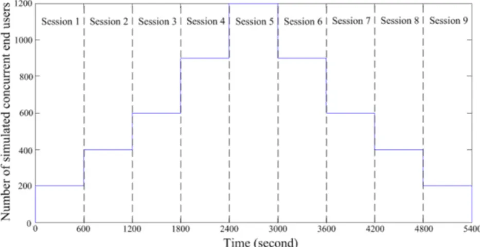
In the first trial, we test the primarily ‘‘browsing’’ workload using nine sessions: the first five sessions stepwise increase the number of simulated end users to initiate scaling up and the remaining four sessions gradually decrease this number to trigger scaling down, as shown inFig. 9(a). This variance of end user numbers denotes the changing workload volume, and the ‘‘thinking time’’ between two requests randomly varies between 0 and 1 s. More concretely, the first session is generated at time
=
0 s and lasts 600 s. During this period, the application is monitored once every 60 s andFig. 9(b) displays 10 observed arrival rates of incoming requests. These observed values can be used to derive the meanλ
mand varianceλ
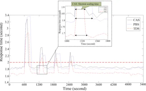
vof the request’s interarrival time.Fig. 10demonstrates the fluctuation of the end-to-end response time observed in the trial of the ‘‘browsing’’ workload. In the first five sessions, the response time is violated whenever the active session number is increased. For instance, when the session number is increased to 400 at time
=
600 s and saturates two Service tiers. The scaling up is triggered and two Tomcat and one Apache servers are added. The violation typically lasts for 1 or 2 min because the addition of new servers consumes some time. By contrast, in the sixth to ninth sessions, the CAS algorithm scales down the application while meeting the required response time.Result. When the workload volume increases, the CAS algorithm can scale up the application to restore the requested response time within 1 or 2 min. On the other hand, the algorithm can scale down the application when the workload volume decreases, while maintaining the response time target.
6.2.2. Scaling for changing workload types
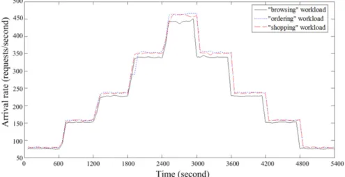
We repeat the last section’s trial to test all three types of workloads, and their observed arrival rates are shown inFig. 11.
Although these rates are similar to each other, workloads of different type stress different tiers of the application.
Given the above workloads,Fig. 12shows that the CAS algo-rithm can scale up and down the application to meet the required response time for the ‘‘ordering’’ and ‘‘shopping’’ workload. More-over,Fig. 13shows the number of servers deployed for each work-load to support different session work-loads. This number adapts to changes in workload types. For example, in most cases of scal-ing up (down) for the ‘‘browsscal-ing’’ workload, the tiers of Tomcat and Apache are saturated or idle and the number of these servers changes with the session number (Fig. 13(a)). By contrast, the MySQL Slave tier is influenced significantly by the session num-ber in the ‘‘ordering’’ workload (Fig. 13(b)). Note that only three types of server, namely Tomcat, Apache and MySQL Slave, are listed because the number of other types of server does not change due to their replication and resource constraints. In addition,Fig. 14
presents the total cost of deploying these servers and that this cost is always kept within the budget.
Result. Our CAS algorithm is able to adapt with different types of workload and identify the bottleneck tiers for each scaling. When the scaling is performed, only the bottleneck tiers are scaled up and down to maintain the response time target.
6.3. Comparison with existing scaling techniques
This section shows the effectiveness of our CAS algorithm in scaling on response time (Section6.3.2) and cost-efficient services (Section6.3.3).
6.3.1. Two categories of existing scaling technique
Typically, existing scaling techniques can be divided into two categories.
In the first category, applications are scaled using pre-defined polices [1,11–13]. These scaling algorithms can be termed Policy-based scaling (PBS), and are used by many mainstream cloud providers such as Amazon WS [1] and Rightscale [11]. In the experiment, if the CPU utilisation of one type of server (e.g., Apache or Tomcat) is larger than 80% for 2 min, one or more additional
(a) Nine sessions and their number of concurrent end users.
(b) Requests’ arrival rate.
Fig. 9. Nine simulated sessions and observed request arrival rate of the ‘‘browsing’’ workload.
Fig. 10. The end-to-end response time in the trial of the ‘‘browsing’’ workload.
servers is added. On the other hand, if this utilisation is less than 50% for 2 min, redundant servers are removed.
In the second category, an application is modelled by a network of queueing models including single or multiple tiers of servers. Each server’s capacity is then analysed using theG
/
G/
1 model. Subsequently, each tier’s required server number is calculated by breaking the application’s end-to-end response time into per-tierresponse times. This type of scaling techniques [4–10,15,39], therefore, is termed Tier-Dividing Scaling (TDS). The TDS algorithm applies worst-case capacity estimation to deploy sufficient servers capable of handling the peak workload. In the experiment, the end-to-end response time (i.e., 2.0 s) is broken down into three per-tier response times, which are 20%, 40% and 40% for the tiers of Apache, Tomcat and MySQL, respectively.