Continuously Maintaining Quantile Summaries of the Most Recent N Elements
over a Data Stream
Xuemin Lin
University of New South Wales
Sydney, Australia
Hongjun Lu
Hong Kong University of Sci. & Tech.
Hong Kong
Jian Xu
University of New South Wales
Sydney, Australia
Jeffrey Xu Yu
Chinese University of Hong Kong
Hong Kong
Abstract
Statistics over the most recently observed data elements are often required in applications involving data streams, such as intrusion detection in network monitoring, stock price prediction in financial markets, web log mining for access prediction, and user click stream mining for per-sonalization. Among various statistics, computing quan-tile summary is probably most challenging because of its complexity. In this paper, we study the problem of contin-uously maintaining quantile summary of the most recently observedNelements over a stream so that quantile queries can be answered with a guaranteed precision ofN. We developed a space efficient algorithm for pre-defined N that requires only one scan of the input data stream and O(log(2N)
+
1
2)space in the worst cases. We also devel-oped an algorithm that maintains quantile summaries for most recentNelements so that quantile queries on any most recentnelements (n≤N) can be answered with a guaran-teed precision ofn. The worst case space requirement for this algorithm is onlyO(log2(2N)). Our performance study
indicated that not only the actual quantile estimation error is far below the guaranteed precision but the space require-ment is also much less than the given theoretical bound.
1
Introduction
Query processing against data streams has recently re-ceived considerable attention and many research break-throughs have been made, including processing of relational type queries [4, 6, 8, 15, 20], XML documents [7, 14], data mining queries [3, 16, 22], v-optimal histogram main-tenance [12], data clustering [13], etc. In the context of data streams, a query processing algorithm is considered efficient if it uses very little space, reads each data element just once, and takes little processing time per data element. Recently, Greenwald and Khanna reported an interesting work on efficient quantile computation [10]. Aφ-quantile (φ ∈ (0,1]) of an ordered sequence of N data elements is the element with rankφN. It has been shown that in
order to compute exactly theφ-quantiles of a sequence of N data elements with onlypscans of the data sequence, any algorithm requires a space ofΩ(N1/p)[19]. While quite a lot of work has been reported on providing approximate quantiles with reducing space requirements and one scan of data [1, 2, 17, 18, 9], techniques reported in [10] (Re-ferred as GK-algorithm hereafter) are able to maintain an -approximate quantile summary for a data sequence ofN elements requiring onlyO(1log(N))space in the worst case and one scan of the data. A quantile summary is -approximate if it can be used to answer any quantile query within a precision of N. That is, for any given rankr, an-approximate summary returns a value whose rankris guaranteed to be within the interval [r−N,r+N].
While quantile summaries maintained by GK-algorithm have their applications, such summaries do not have the concept of aging, that is, quantiles are computed for all Ndata elements seen so far, including those seen long time ago. There are a wide range of applications where data ele-ments seen early could be outdated and quantile summaries for the most recently seen data elements are more important. For example, the top ranked Web pages among most re-cently accessedNpages should produce more accurate web page access prediction than the top ranked pages among all pages accessed so far as users’ interests are changing. In fi-nancial market, investors are often interested in the price quantile of the most recent N bids. Detar et. al. con-sidered such a problem of maintaining statistics over data streams with regard to the lastN data elements seen so far and referred to it as the sliding window model [5]. However, they only provided algorithms for maintaining aggregation statistics, such as computing the number of1’s and the sum of the lastN positive integers. Apparently, maintaining or-der statistics (e.g. quantile summary) is more complex than those simple aggregates. Several approximate join process-ing [4] and histogram techniques [11] based on the slidprocess-ing window model have also been recently reported but they are not relevant to maintaining order statistics.
space-efficient one-pass quantile summaries over the most recentNtuples seen so far in data streams. Different from the GK-algorithm where tuples in a quantile summary are merged based on capacities of tuples when space is needed for newly arrived data elements, we maintain quantile sum-mary in partitions based on time stamps so that outdated data elements can be deleted from the summary without af-fecting the precision. Since quantile information is local to each partition, a novel merge technique was developed to produce an-approximate summary from partitions for all N data elements. Moreover, we further extended the tech-nique to maintain a quantile summary for the most recent N data elements in such a way that quantile estimates can be obtained for thenmost recent elements for anyn≤N.
To the best of our knowledge, no similar work has been reported in the literature. The contribution of our work can be summarized as follows.
• We extended the sliding window model to an n-of-N model. Under the sliding window model, quan-tile summaries are maintained for theN most recently seen elements in a data stream. Under the n-of-N model, quantile summary with a sliding windowNcan produce quantile estimates for anyn (n ≤ N) most recent elements. In other words, the sliding window model can be viewed as a special case of then-of-N model.
• For the sliding window model, we developed a one-pass deterministic -approximate algorithm to main-tain quantiles summaries. The algorithm requires a space ofO(log(2N)+12).
• For the generaln-of-N model, we developed another one-pass deterministic approximate algorithm that re-quires a space ofO(12log2(N)). The algorithm is -approximate for everyn≤N.
• The technique developed to merge multiple -approximate quantile summaries into a single -approximate quantile summary can be directly used for distributed and parallel quantile computation.
The rest of this paper is organized as follows. In sec-tion 2, we present some background informasec-tion in quan-tile computation. Section 3 and 4 provide our algorithms for the sliding window model and the n-of-N model, re-spectively. Discussions of related work and applications are briefly presented in section 5. Results of a comprehen-sive performance study are discussed in section 6. Section 7 concludes the paper.
2
Preliminaries
In this section, we first introduce the problem of quantile computation over a sequence of data, followed by a num-ber of computation models. Finally we review some most closely related work.
12
t1
10
t2
11
t4
1
t5
10
t6
11
t7
9
t9
7
t8
6
t10
8
t12
4
t11
11
13 t
5
t14
2
t15
3 10
3 t t0
Figure 1. a data stream with arrival time-stamps
2.1
Quantile and Quantile Sketch
In this paper, for notation simplification we will always assume that a data element is a value and an ordered se-quence of data elements in quantile computation always means an increasing ordering of the data values. Further-more, we always useN to denote the number of data ele-ments.
Definition 1 (Quantile). Aφ-quantile (φ∈(0,1]) of an or-dered sequence ofNdata elements is the element with rank
φN. The result of a quantile query is the data element for a given rank.
Example 1. Figure 1 shows a sample sequence of data
gen-erated from a data stream where each data element is rep-resented by a value and the arrival order of data elements is from left to right. The total number of data elements in the sequence is 16. The sorted order of the sequence is 1, 2,3,4,5,6,7,8,9,10,10,10,11,11,11,12. So, 0.5-quantile returns the element ranked 8 (=0.5*16), which is 8; and 0.75-quantile returns an element 10 which ranks 12 in the sequence.
Munro and Paterson showed that any algorithm that computes the exactφ-quantiles of a sequence ofN data el-ements with onlypscans of the data sequence requires a space ofΩ(N1/p)[19]. In the context of data streams, we are only able to see the data once. On the other hand, the size of a data steam is theoretically infinite. It becomes im-practical to compute exact quantile for data streams. For most applications, keeping an quantile summary so that quantile queries can be answered with bounded errors is in-deed sufficient.
Definition 2 (-approximate). A quantile summary for a
data sequence of N elements is-approximate if, for any given rankr, it returns a value whose rankris guaranteed to be within the interval [r−N,r+N].
Generally, a quantile summary may be in any form. Def-inition 2 does not lead to a specific query algorithm to find a data element from an-approximate summary within the precision ofN. To resolve this, a well-structured -approximate summary is needed to support -approximate quantile queries. In our study, we use quantile sketch or sketch for brevity, a data structure proposed in [10] as the quantile summaries of data sequences.
Definition 3 (Quantile Sketch). A quantile sketchSof an ordered data sequenceDis defined as an ordered sequence of tuples {(vi, r−i , r
+
i ) : 1 ≤ i ≤ m} with the following properties.
1. Eachvi∈D.
2. vi ≤vi+1for1≤i≤m−1.
3. r−i < r−i+1for1≤i≤m−1.
4. For1≤i≤m,r−i ≤ri≤r+i whereriis the rank of viinD.
Example 2. For the sequence of data shown in Figure 1,
{(1,1,1), (2,2,9), (3,3,10),(5,4,10),(10,10,10),(12,16,16)}is an example quantile sketch consisting of 6 tuples.
Greenwald and Khanna proved the following theorem:
Theorem 1. For a sketchSdefined in Definition 3, if: 1. r+1 ≤N+ 1,
2. r−m≥(1−)N,
3. for2≤i≤m,ri+ ≤r−i−1+ 2N.
thenSis-approximate. That is, for eachφ∈(0,1], there is a(vi, r−i , r
+
i )inSsuch thatφN −N ≤r−i ≤r
+
i ≤
φN+N.
Theorem 1 states that for each rankr, we are able to find a tuple(vi, r−i , r
+
i )from such an-approximate sketch by a linear scan, such that the rankriofviis within the precision ofN, that is,r−N ≤ri ≤r+N. In the rest of paper, we will use the three conditions in Theorem 1 to define an -approximate sketch.
Example 3. It can be verified that the sketch provided in
Example 2 is 0.25-approximate with respect to the data stream in Figure 1. On the other hand, the sketch{(1,1,1), (3,2,10), (10,10,10), (12, 16, 16)}is0.2813-approximate.
Note that the three conditions presented in Theorem 1 are more general than those originally in [10] due to our applications to the most recentN elements. However, the proof techniques in Proposition 1 and Corollary 1 [10] may lead to a proof of Theorem 1; we omit the details from this paper.
2.2
Quantile Sketches for Data Streams
Quantile summaries, or in our case, quantile sketch can be maintained for data streams under different computation models.
Data stream model. Most previous work are working with
the data stream model. That is, a sketch is maintained for allNdata items seen so far.
Sliding window model. Under sliding window model, a
sketch is maintained for the most recently seenN data ele-ments. That is, for anyφ∈(0,1], we computeφ-quantiles against theN most recent elements in a data stream seen so far, whereN is a pre-fixed number.
n-of-N model. Under this model, a sketch is maintained
forN most recently seen data elements. However, quantile queries can be issued against anyn≤N. That is, for any φ∈(0,1]and anyn≤N, we can returnφ-quantiles among thenmost recent elements in a data stream seen so far.
Consider the data stream in Figure 1.
• Under the data stream model, since a sketch is main-tained for all N data elements seen so far, a 0.5-quantile returns 10 at timet11, and 8 at timet15.
• With the widthN of the sliding window being 12, a 0.5-quantile returns 10 at timet11, and 6 at timet15, which is ranked sixth in the most recentN = 12 ele-ments.
• Assume that the sketch is maintained sincet0with the n-of-N model, at timet15, quantile queries can be an-swered for any1≤n ≤16. A 0.5-quantile returns 6 forn= 12and 3 forn= 4.
It can be seen that different sketches have different ap-plications. For example, in databases, a sketch maintained under the data stream model is useful for estimating the sizes of relational operations which is required for query optimization. For a Web server, it is more appropriate to maintain a sketch on accessed Web pages under the sliding window model so that a page access prediction for cache management can be based on most recent user access pat-terns. In a security house, a sketch of bid/ask prices main-tained under the n-of-N model is more appropriate so that it can answer quantile queries from clients with different investment strategies.
2.3
Maintaining
-Approximate Sketches
In our study, we are interested in deterministic tech-niques with performance guarantees. Such algorithms are only available under the data stream model or the model of disk residence data.
Manku, Rajagoipalan and Lindsay [17] developed the first deterministic one-scan algorithm, with poly-logarithmic space requirement, for approximately com-puting φ-quantiles with the precision guarantee of N. Greenwald-Khanna algorithm [10] reduced the space com-plexity toO(1log(N))for a data stream withNelements seen so far. The GK-algorithm [10] maintains a sketch by one-pass scan of a data stream to approximately an-swer quantile queries. A generated sketch is guaranteed -approximate.
For presentation simplification, the GK-algorithm uses two parameters gi and∆i to controlri− andr
+
i for each tuple(vi, r−i , r
+
i )in a generated sketch such that for eachi,
• j≤igj≤ri ≤
j≤igj+ ∆i,
• r−i =
j≤igj, (a)
• r+i =
j≤igj+ ∆i. (b)
The GK-algorithm maintains the following invariants to en-sure that a generated sketch{(vi, r−i , r
+
i ) : 1 ≤i≤m}is -approximate.
Invariant 1: For2≤i≤m,gi+ ∆i<2N.
Invariant 2: v1 is the first element in the ordered data stream.
Invariant 3: vn is the last element in the ordered data stream.
2.4
Challenges
Note that in the sliding window model, the actual con-tents of the most recentNtuples change upon new elements arrive, thoughNis fixed. This makes the existing summary techniques based on a whole dataset not trivially applicable.
Example 4. GK-algorithm generates the following sketch
regarding the data stream as depicted in Figure 1 if= 0.5.
{(1,1,1),(10,9,9),(12,16,16)}
The data elements involved in the sketch are1,10, and12. If we want to compute the quantiles against the most recent 4elements (i.e.,2,3,4,5), this sketch is useless.
Clearly, it is desirable that the data elements outside a sliding window should be removed from our considerations. As the contents in a sliding window continuously change upon new elements arrive, it seems infeasible to remove the exact outdated elements without using a space of O(N). Therefore, the challenges are to develop a space-efficient technique to continuously partition a data stream and then summarize partitions to achieve high approximate accuracy. The quantile summary problem forn-of-N model seems even harder.
3
One-Pass Summary for Sliding Windows
In this section, we present a space-efficient summary algorithm for continuously maintaining an -approximate sketch under a sliding window. The basic idea of the al-gorithm is to continuously divide a stream into the buckets based on the arrival ordering of data elements such that:
• Data elements in preceding buckets are generated ear-lier than those in later buckets.
• The capacity of each bucket is N2 to ensure -approximation.
• The algorithm issues a new bucket only after the pre-ceding blocks are full.
• For each bucket, we maintain an 4-approximate sketch continuously by GK-algorithm instead of keeping all data elements.
• Once a bucket is full, its 4-approximate sketch is com-pressed into an 2-approximate sketch with a space of O(1
).
• The oldest bucket is expired if currently the total num-ber of elements isN+ 1; consequently the sketch of the oldest bucket is removed.
• Merge local sketches to approximately answer a quan-tile query.
Figure 2 illustrates the algorithm. Note that GK-algorithm has been applied to our algorithm only because it has the smallest space guarantee among the existing techniques. Our algorithm will be able to accommodate any new algo-rithms for maintaining an-approximate sketch.
The rest of the section is organized as follows. We successively present our novel merge technique, compress technique, sketch maintenance algorithm, and query algo-rithm.
3.1
Merge Local Sketches
Suppose that there areldata streamsDifor1 ≤i≤l, and each Di has Ni data elements. Further suppose that each Si (1 ≤ i ≤ l) is an η-approximate sketch ofDi. In this subsection, we will present a novel technique to merge these l sketches such that the merged sketch is η-approximate with respect to∪li=1Di. This technique is the key to ensure-approximation of our summary technique, although used only in the query part.
Algorithm 1 depicts the merge process. EachSi(for1≤ i≤l) is represented as{(vi,j, ri,j−, r
+
i,j) : 1≤j ≤ |Si|}. Algorithm 1 Merge
Input:
{(Si, Ni) : 1≤i≤l}; eachSiisη-approximate. Output:
Smerge. Description:
1: Smerge:=∅;r−0 := 0;k:= 0;
2: for1≤i≤ldo
3: ri,−0:= 0;
4: end for
5: while∪li=1Si=∅do
6: choose the tuple (vi,j, r−i,j, r
+
i,j) with the smallest vi,j;
7: Si:=Si− {(vi,j, ri,j−, r
+
i,j)};
8: k:=k+ 1;vk :=vi,j;
9: rk−:=r−k−1+ri,j− −ri,j−−1;
10: ifk= 1then
11: rk+:=ηki=1Ni+ 1
12: else
13: rk+:=rk−−1+ 2η
k
i=1Ni;
14: Smerge:=Smerge∪ {(vk, rk−, rk+)}.
15: end if
16: end while
We first prove thatSmergeis a sketch of∪li=1Di. This is an important issue. Suppose that for a given rankr, we can find a tuple(vk, r−k, r
+
k)inSmergesuch thatr−N ≤ r−k ≤r
+
k ≤r+N. There is no guarantee thatrk(the rank ofvk) is within[r−N, r+N]unlessrk is betweenr−k andrk+.
2Ν ε
elements 2Ν ε
elements 2Ν ε
elements 2εΝelements
ε/2
compressed −approximate sketch in each bucket
expired bucket
the most recent N elements
current bucket
GK
Lemma 1. Suppose that there are l data streams Di for 1 ≤ i ≤ l and eachDi hasNi data elements. Suppose that each Si (1 ≤ i ≤ l) is anη-approximate sketch of Di. Then, Smerge generated by the algorithm Merge on
{Si: 1≤i≤l}is a sketch of∪li=1Diwhich has
l
i=1|Si| tuples.
Proof. It is immediate thatSmergehas
l
i=1|Si|tuples. Based on the algorithm Merge, the first 3properties in the sketch definition can be immediate verified. We need only to prove that for each(vk, r−k, r+k) ∈ Smerge,r−k ≤ rk≤r+k whererkis the rank ofvk in the ordered∪ki=1Di.
For each(vk, r−k, r
+
k) ∈ Smerge,(vi,jk,i, r−i,jk,i, r
+
i,jk,i) denotes the last tuple ofSi(1≤i≤l) merged intoSmerge no later than obtaining(vk, rk−, r
+
k). Note that ifjk,i = 0 (i.e. no tuple in Si has been merged yet), then we make vi,0=−∞andr−i,0=ri,0=ri,+0= 0.
It should be clear thatvk ≥vi,jk,i for1 ≤i≤l.
Con-sequently,rk ≥
l
i=1ri,jk,i ≥
l
i=1r−i,jk,i. According to the algorithm Merge (line9), it can be immediately verified that for eachk,
rk−= l
i=1
r−i,jk,i. (1)
Thus,rk ≥rk−.
Now we prove thatrk≤r+k fork≥2, as it is immediate thatr1 ≤r+1. Suppose thatrk =
l
i=1pi where eachpi denotes the number of elements fromSinot aftervk in the merged stream. Assume vk is from streamDα. Clearly, pα=rα,jk,α ≤rα,j+ k,α ≤r−α,jk,α−1+ 2ηNα.
For each pi = 0 (i = α), note that r−i,jk,i + 2ηNi ≥ r+i,jk,i+1. Ifpi > ri,j−k,i+ 2ηNi, thenrk> r−i,ki+ 2ηNi≥ ri,ki+1; consequently,(vi,jk,i, ri,j−k,i, r
+
i,jk,i)is not the last tuple fromSi merged intoSmerge beforevk. Contradict! Therefore,pi≤r−i,jk,i + 2ηNifor eachpi= 0(i=α).
By the algorithm Merge (line 9), fork ≥ 2,rk−−1 =
l
i=1,i=αr−i,jk,i+rα,j− k,α−1. Thus,rk ≤r+k.
Theorem 2. Suppose that there areldata streamsDi for 1 ≤ i ≤ l and eachDi hasNi data elements. Suppose that each Si (1 ≤ i ≤ l) is anη-approximate sketch of Di. Then, Smerge generated by the algorithm Merge on
{Si: 1≤i≤l}is anη-approximate sketch of∪li=1Di. Proof. The property 1 and property 3 in the definition of “η-approximate” (in Theorem 1) are immediate. From the equation (1), the property 2 immediately follows.
3.2
Sketch Compress
In this subsection, we will present a sketch compress al-gorithm to be used in our sketch construction alal-gorithm. The algorithm is outlined in Algorithm 2. It takes an ξ2 -approximate sketch of a data set with N elements as an input, and produces anξ-approximate sketch with at most
1
ξ+ 2tuples.
Algorithm 2 Compress Input:
an2ξ-approximate sketchS;
Output:
anξ-approximate sketchScomd with at most1ξ+ 2 tuples
Description:
1: Scomd:=∅;
2: Add toScomdthe first tuple ofS;
3: for 1≤j≤ 1ξ do
4: letsbe the first tuple(vkj, r−kj, r
+
kj)inS such that jξN −ξN2 ≤r−kj ≤r+kj ≤jξN+ξN2 ;
5: Scomd:=Scomd∪ {s}.
6: end for
7: Add the last tuple ofStoScomd.
Note thatS is an ordered sequence of tuples. In Algo-rithm 2,sis the first tuple satisfying the condition from the beginning ofS. Clearly, the algorithm can be implemented in a linear time with respect to the size ofS.
Suppose thatScomd has the same ordering asS. Then it can be immediately verified thatScomdis a sketch. Ac-cording to the condition given in line 4 in Algorithm 2, the property 3 in the definition (in Theorem 1) ofξ-approximate is immediate. Therefore,Scomdis anξ-approximate sketch of the data stream.
Theorem 3. Suppose that S is an ξ2-approximate sketch. Then,Scomdgenerated by the algorithm Compress onS is ξ-approximate, which has at most1ξ+ 2tuples.
Note that regarding the same precision guarantee, our new compress technique takes about half of the number of tuples given by the compress technique in [10].
3.3
Sketch Construction and Maintenance
We are now ready to present our algorithm that continu-ously maintains a sketch to answer approximately a quantile query under the sliding window model. According to The-orem 2, in our sketch maintenance algorithm we need only to maintain a good approximate sketch for each bucket. The algorithm, outlined in Algorithm 3, follows the scheme as depicted in Figure 2.
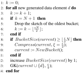
Note that in each bucket, the algorithm keeps 1) its sketch, 2) its time-stamp, and 3) the number of elements contained in the bucket. The algorithm is quite straightfor-ward. For a new data item, if the total numberkof elements remained in our consideration is over the size of the sliding windowN, the sketch for the oldest bucket is dropped (line 4-6). If the current bucket size exceeds 2N, its corre-sponding sketch will be compressed to a sketch with a con-stant numberO(1)of tuples (line 9) and a new bucket is cre-ated as the current bucket (line 10). The new data element is always inserted into a sketch of the current bucket by GK-algorithm for maintaining 4-approximation (line 13). Note
Algorithm 3 SW Description:
1: k:= 0;
2: for all new generated data elementddo
3: k:=k+ 1;
4: if k=N+ 1 then
5: Drop the sketch of the oldest bucket;
6: k:=k− N2 ;
7: end if
8: if BucketSize(current)≥ 2Nthen
9: Compress(current,ξ=2);
10: current:=N ewBucket();
11: end if
12: increaseBucketSize(current)by1;
13: GK(current∪ {d},4); 14: end for
that in Algorithm 3, we use current to represent a sketch for the current bucket, and we also record the number of elements in the current bucket as BucketSize(current). Note that when a new bucket is issued (line 10), we initialize only its sketch (current) and its bucket size (BucketSize), as well as assign the the time-stamp of the new bucket as the arrival time-stamp of the current new data element.
From the algorithm Compress, it is immediate that the local sketch for each bucket (except the current one) is 2 -approximate restricted to their local data elements, while the current (last) one is 4-approximate. Further, the follow-ing space is required by the algorithm SW.
Theorem 4. The algorithm SW requiresO(log(2N)+12)
space.
Proof. The sketch in each bucket produced by the algorithm GK takesO(log(2N))space which will be compressed to a space of O(1)once the bucket is full. Clearly, there are O(1
)buckets. The theorem immediately follows.
3.4
Querying Quantiles
In this subsection, we present a new query algorithm which can always answer a quantile query within the preci-sion ofN, in light of Theorem 2. Note that in the algorithm SW, the numberNof data elements in the remaining buck-ets may be less thanN- the maximum difference (N−N) is N2 −1. Consequently, after applying the algorithm Merge on the remaining local sketches, we can guarantee only thatSmergeis an 2-sketch of theN element. There is even no guarantee thatSmergeis a sketch of theN ele-ments.
1, 2, 3, 4, 5, 6, 7, 8, 9
Expired Current Figure 3.= 1andN= 8
For example, suppose that a stream arrives in the order 1,2,3,4, ...,9as depicted in Figure 3. Upon the element
9 arrives, the first bucket (with4elements) is expired and its local sketch is dropped. The local 2-approximate sketch could be (5,1,1) and(7,3,3) for the second bucket and (9,1,1)for the current bucket. After applying the algorithm Merge on them, the first tuple inSmergeis(5,1,3.5). Note that in this example, the most recent8 elements should be 2,3,4,5, ... 9, and the rank of5is 4. As the rank 4is not between1and3.5,Smerge is not a sketch for these 8 elements.
To solve this problem, we use a “lift” operation, outlined in Algorithm 4, to lift the value of ri+ by N2 for each tuplei.
Algorithm 4 Lift Input:
S,ζ;
Output:
Slif t; Description:
1: Slif t:=∅;
2: for all tupleai= (vi, ri−, r
+
i )inSdo
3: updateaibyri+:=r
+
i + ζ
2N)
4: insertaiintoSlif t
5: end for
Theorem 5. Suppose that there is a data steamDwithN elements and there is an ζ2-approximate sketchSof the most recent N elements in D where 0 ≤ N −N ≤ ζ2N. Then,Slif t generated by the algorithm Lift on S is an ζ-approximate sketch ofD.
Proof. We first prove thatSlif tis a sketch ofD. Suppose that:
• (vi, r−i , r
+
i + ζ
2N)is a tuple inSlif tand(vi, r−i , r
+
i ) is a tuple inS;
• riis the rank ofviin the orderedNdata items;
• riis the rank ofviin the orderedD.
Clearly,ri ≥ ri ≥ ri−, andri ≤ ri+ζ2N. AsS is a sketch of theN data items,ri ≤ri+. Consequently,ri ≤ r+i +
ζ
2N. The other sketch properties ofSlif t can be immediately verified.
Theζ-approximation ofSlif t can be immediately veri-fied from the definition (in Theorem 1).
Our query algorithm is presented in Algorithm 5. According to the theorems 1, 2, and 5, the algorithm SW Query is correct; that is, for each rank r = φN (φ∈(0,1]) we are always able to return an elementvisuch that|r−ri| ≤N.
3.5
Query Costs
Note that in our implementation of the algorithm SW Query, we do not have to completely implement the
Algorithm 5 SW Query
Step 1: Apply the algorithm Merge (η =/2) to the local sketches to produce a merged 2-approximate scheme Smergeon the non-dropped local sketches.
Step 2: Generate a sketchSlif t fromSmergeby the algo-rithm Lift by askingζ=.
Step 3: For a given rankr = φN, find the first tuple (vi, ri−, r
+
i )inSlif tsuch thatr−N ≤ri− ≤r
+
i ≤ r+N. Then return the elementvi.
algorithm Merge and the algorithm Lift, nor materialize the Smerge and Slif t. The three steps in the algorithm SW Query can be implemented in a pipeline fashion:
Once a tuple is generated in the algorithm Merge, it passes into Step 2 for the algorithm Lift. Once the tuple is lifted, it passes to the Step 3. Once the tuple is qualified for the query condition in Step 3, the algorithm terminates and returns the data element in the tuple.
Further, the algorithm Merge can be run in a way similar to thel-way merge-sort fashion [21]. Consequently, the algo-rithm Merge runs in aO(mlogl)wheremis the total num-ber of tuples in thel sketches. Since the algorithm Merge takes the dominant costs, the algorithm SW Query also runs in timeO(mlogl).
Note that in our algorithms, we apply GK-algorithm, which records(vi, gi,∆i)instead of(vi, ri−, r
+
i )for each i. In fact, the calculations ofr−i andr+i according to the equations (a) and (b) can be also pipelined with the steps 1-3 of the algorithm SW Query. Therefore, this does not affect the time complexity of the query algorithm.
4
One-Pass Summary under n-of-N
In this section, we will present a space-efficient algo-rithm for summarising the most recent N elements to an-swer quantile queries for the most recentn(∀n≤N) ele-ments.
As with the sliding window model, it is desirable that a good sketch to support then-of-N model should have the properties:
• every data element involved in the sketch should be included in the most recentnelements;
• to ensure-approximation, a sketch to answer a quan-tile query against the most recentnelements should be built on the most recentn−O(n)elements.
Different from the sliding window model, in the n-of-N modelnis an arbitrary integer between1andN. Conse-quently, the data stream partitioning technique developed in the last section cannot always accommodate such requests; for instance whenn <N2 , Example 4 is also applicable.
In our algorithm, we use the EH technique [5] to partition a data stream. Below we first introduce the EH partitioning technique.
4.1
EH Partitioning Technique
In EH, each bucket carries a time stamp which is the time stamp of the earliest data element in the bucket. For a stream withN data elements, elements in the stream are processed one by one according to their arrival ordering such that EH maintains at most λ1+ 1 “i-buckets” for eachi. Here, ani-bucket consists ofidata elements con-secutively generated. EH proceeds as follows.
Step 1: When a new element e arrives, it creates a 1-bucket for eand the time-stamp of the bucket is the time-stamp ofe.
Step 2: If the number of1-buckets is full (i.e.,λ1+ 2), then merge the two oldesti-buckets into ani+1-bucket (carry the oldest time-stamp) iteratively fromi = 1. At every leveli, such merge is done only if the number of buckets becomes1λ+ 2; otherwise such a merge iteration terminates at leveli.
Merge Starts
e1 e2 e3 e4 1−buckets
Merge Starts e
6
e4 e5
e3
e2
e1
Merge Starts
e1 e2 e3 e4 e5 e6 e7 e8 10
e e1 e2 e3 e4 e5 e6 e7 e8 e9
Merge Starts
e1 e2 e3 e4 e5 e6 e7 e8 e9 e10 4−bucket
e1 e2 e3 e4 e5 e6 e7 e8 e9 e10
2−bucket
a data stream
Figure 4. EH Partition:λ= 0.5
Figure 4 illustrates the EH algorithm for 10 elements whereλ= 12and eacheiis assumed to have the time stamp i. The following theorems are immediate [5]:
Theorem 6. ForNelements, the number of buckets in EH is alwaysO(log(λλN)).
Theorem 7. The numberNof elements in a bucketbhas the property thatN−1 ≤λNwhereN is the number of elements generated after all elements inb.
4.2
Sketch Construction
In our algorithm, for each bucketbin EH, we record 1) a sketchSbto summarize the data elements from the earliest element inbup to now, 2) the numberNbof elements from the earliest element in bup to now, and 3) the time-stamp tb.
Once two bucketsbandb are merged, we keep the in-formation ofbifbis earlier thanb. Figure 5 illustrate the algorithm.
We present our algorithm below in Algorithm 6. Note that to ensure-approximation, we chooseλ=
+2 in our algorithm to run the EH partitioning algorithm, and GK-algorithm is also applied to maintaining an 2-approximate sketch.
Algorithm 6 nN
Upon a new data elementearrives at timet,
Step 1 - create a new sketch: Record a new1-buckete, its time stampteast, andNe= 0. Initialize a sketchSe. Step 2 - drop sketches: If the number of1-buckets is full (i.e.,λ1+ 2), then do the following iteratively from i= 1tilljwhere the current number (before this new element arrives) ofj-buckets is not greater than1λ.
• get the two oldest bucketsb1 andb2 among the i-buckets; and then
• dropb1andb2from thei-th bucket list; and then
• drop the sketchSb2 (assume theb1is older than
b2); and then
• addb1 together with its time stamp intoi+
1-buckets list.
Scan the sketch list from oldest to delete the expired bucketsb- (Sb,Nb,tb); that isNb≥N.
Step 3 - maintain sketches: for each remaining sketchSb, adde intoSb by GK-algorithm for 2-approximation andNb:=Nb+ 1.
By Theorem 6, the algorithm nN maintainsO(log(N)) sketches, and each sketch requires a space of O(log(N)) according to GK-algorithm. Consequently, the algorithm nN requires a space ofO(log2(2N)).
4.3
Querying Quantiles
In this subsection, we show that we can always get an -approximate sketch among the sketches maintained Al-gorithm 6 to answer a quantile query for the most recent n(∀n ≤ N) elements. Our query algorithm, described in Algorithm 7 consists of3steps. First, we choose an appro-priate sketch among the maintained sketch. Then, we use the algorithm Lift, and finally check the query condition.
Theorem 8. Algorithm 7 is correct; that is,
• the algorithm is always able to return a data element;
• the element returned by the algorithm meets the re-quired precision.
Proof. To prove the theorem, we need only to prove that
4−bucket
Sf Se
Sd Sc
Sb Sa
4−bucket
Se Sd
Sc
Sa Sb Sf
Se
2−buckets 1−buckets
e
a c
e d
f
Before insert e
new merged
2−buckets 1−buckets
e
d c b
e
After insert e
a f
b
Figure 5. Algorithm nN:η= 0.5
Algorithm 7 nN Query Input:
Sketches maintained in the algorithm nN whereλ= +2 , n(n≤N), andr=φn(φ∈(0,1]).
Output:
an element v in the most recent n elements such that r−n ≤ r ≤ r+n(r is the rank ofv in the most recentnelements).
Step 1: For a givenn (n ≤ N), scan the sketch list from oldest and find the first sketch Sbn such that
Nbn ≤n.
Step 2: Apply the algorithm Lift toSbnto generateSlif t whereζ=.
Step 3: For a given rank r, find the first tuple (v+
i , r
+
i , r−i )inSlif tsuch that thatr−n≤r−i ≤ r+i ≤r+n. Returnvi.
Slif t is an-approximate sketch of the most recentn ele-ments.
Note that in Algorithm 6, Sbn is maintained, by GK-algorithm for 2-approximation, over the most recentNbn elements.
Case 1: n < Nbn. Suppose thatbn is the bucket in EH, which is just beforebn. Then,Nb
n > nsinceNbn is the
largest number which is not larger than n. Consequently, n−Nbn ≤ Nbn −Nbn −1. According to Theorem 7, n−Nbn ≤2+Nbn. This implies thatn−Nbn<2n; thus
n−Nbn≤
2n (2)
Note that since Theorem 7 also covers an expired bucket, the inequality (2) holds ifSbn is the oldest. Based on the
inequality (2) and Theorem 5, Slif t is an -approximate sketch of the most recentnelements.
Case 2: n = Nbn. It is immediate that Slif t is an -approximate sketch of the most recentnelements according to Theorem 5. In fact, in this case we do not have to use the algorithm Lift; however for the algorithm presentation sim-plification, we still include the operation for this case.
Note that we can also apply a pipeline paradigm to the steps 2 and 3, in a way similar to that in section 3.5, to speed-up the execution of Algorithm 7. Consequently, Al-gorithm 7 runs inO(log(N))time.
5
Discussions and Applications
The algorithm developed by Alsabti-Ranka-Singn (ARS) [2] is to compute quantiles approximately by one scan of datasets. Although this partition based algorithm was originally designed for disk-resident data, it may be modified to support the sliding window. However, this algo-rithm requires a space ofΩ(
N
a merge technique in the algorithm ARS but it was specif-ically designed to support the algorithm ARS; for instance, it does not support the sketches generated by GK-algorithm to retain-approximation. Therefore, the merge technique in the algorithm ARS is not applicable to our algorithm SW. In the next section, we will also compare the modified ARS with the algorithm SW by experiments.
Note that in applying the EH partitioning technique [5], we may have another option - maintaining only local sketches for each bucket and then merge two local sketches when their corresponding buckets are merged. Though this can retain-approximation, we found that in some cases we have to keep all the tuples from two buckets; this prevent us to work out a good space guarantee. In the next section, we will report the space requirements of a heuristic based on this option.
Now we show that the techniques developed in this pa-per can be immediately applied to other important quantile computation problems. Below we list three of such applica-tions.
Distributed and Parallel Quantile Computation: In many applications, data streams are distributed. In light of our merge technique and Theorem 2, we need only to main-tain a local-approximate sketch for each local data stream to ensure the global-approximation.
Most Recent T Period: In some applications, users may be
interested in computing quantiles against the data elements in the most recentT period. The algorithm nN may be im-mediately modified to serve for this purpose. In the modi-fication, to ensure-approximation we need only to change the expiration condition of a sketch: a sketch is expired if its time stamp is expired. Then we use the oldest remaining sketch to answer a quantile query. The space requirement is O(log2(N)
2 )whereN is the maximum number of elements
in aT period. Note that in this application,N is also un-known in eachT; however, it can be-approximated by EH. We omit the details from the paper due to the space limita-tion.
Constrain based Sliding Window: In many applications,
the users may be interested in only the elements meeting some constraints in the most recentNelements. In this ap-plication, we can also modify the algorithm nN to support an-approximate quantile computation for the elements sat-isfying the constraints in the most recentN elements. In the modification of the algorithm nN, we only allow the elements meeting the constraints to be added while each sketch still count the number of elements (even not meeting the constraints) “seen” so far and the number of elements seen so far meeting the constraints. Then, we use the old-est sketch to approximately answer a quantile query. The space requirement isO(log2(2N)). Similar to the most
re-cent T period model, we need to-approximate the number of qualified elements in the most recentNelements.
Notation Definition (Default Values)
N The size of sliding window (800K) The guaranteed precision (0.05) φ (1/q, ...,(q−1)/q)for a givenq Dd Data distribution (Uniform) Qp The query patterns (Random) I The length of a rank interval (N) #Q The number of queries (100,000)
Table 1. System parameters.
6
Performance Studies
In our experiments, we modified ARS-algorithm [2] to support the sliding window model. In our modification, we partition a data stream in the way as shown in [17], which leads to the minimum space requirement. We implemented our algorithms SW and nN, as well as a heuristic - algo-rithm nN’. The algoalgo-rithm nN’ also adopts the EH partition-ing technique; however, in nN’ we maintain local sketches for each bucket in EH, and then use GK-algorithm [10] to merge two local sketches once the corresponding buckets have to be merged. As discussed in the last section, we did not obtain a good bound on the space requirements of nN’.
All the algorithms are implemented using C++. We con-ducted experiments on a PC with an Intel P4 1.8GHz CPU and 512MB memory using synthetic and real datasets.
The possible factors that will affectφ-quantile queries are shown in Table 1 with default values. The parame-ters are grouped in three categories: i) N (window size), (guaranteed precision), andφ(quantiles), ii) data distribu-tions (Dd) to specify the “sortedness” of a data stream, and iii) query patterns (Qp), lengths of rank intervals (I) to be queried, and the number of queries (#Q).
In our experiments, the data distributions (Dd) tested take the following random models: uniform, normal, and exponential. We also examined sorted or partially sorted data streams, such as global ascending, global descending, and partially sorted.
We use the estimation error as the error metrics to eval-uate the tightness ofas an upper-bound. The estimation error is represented as |rM−r|whereris an exact rank to be queried,r is the rank of a returned element, andM is the number of most recent elements to be queried. Here,M is N in a sliding window and isnin then-of-Nmodel.
As for query patterns (Qp), in addition to the random φ-quantile queries, we also consider the80-20rules such as80%of queries will focus on a small rank interval (with lengthI) and20%of queries will access arbitrary ranks.
6.1
Sliding Window Techniques
In this subsection, we evaluate the performance of our sliding window techniques. In our experiments, we exam-ined the average and maximum errors ofφ-quantile queries based on a parameterq, and makeφ-quantiles be in the form of1/q,2/q, ...,(q−1)/q.
SW ARS 0
0.01 0.02 0.03 0.04 0.05 0.06
Avg Estimation Error
ε=0.025 ε=0.05 ε=0.075 ε=0.1
(a) Avg Errors (q= 32)
ε=0.1 ε=0.075 ε=0.05 ε=0.025 0
1000 2000 3000 4000
Space Usage: #tuples
SW ARS
Theoretic Bound of SW
(b) Space Consumption
1 200000 400000 600000 800000 Rank
0.001 0.01 0.1 1 10
Relative Error( error/fi)
SW ARS
(c) Rank vs Errors(= 0.025)
Figure 6. Avg/Max Errors, Space Consumptions, and Rank (sliding window)
Overall Performance. An evaluation of overall
perfor-mance of SW and ARS is shown in Figure 6 for the sliding window modelN. In this set of experiments,N = 800K and a data stream is generated using a uniform distribution with 1000K elements. We tested four differents: 0.1, 0.075,0.05and0.025.
Figure 6 (a) illustrates the average errors when q = 32. It shows that ARS performs similarly to nN regard-ing accuracy. This has been confirmed by a much larger set of queries using another error metrics: relative error (|r−rr|). Figure 6 (c) shows the relative errors of all φ-quantile queries in the form of1/q,2/q, ...,(q−1)/q(∀q∈ [1,800K]when = 0.025. Overall, the relative error de-creases whileqincreases but is not necessarily monotonic. The fluctuations of SW is much smaller than ARS, though their average relative errors are very close.
Uni Norm Exp Sort Rev Block Semi 0
200 400 600 800
Space Usage: #tuples
Figure 7. Space Consumptions vs Distributions
Uni Norm Exp Sort Rev Block Semi 0
0.005 0.01 0.015 0.02 0.025 0.03 0.035 0.04
Estimation Error
Avg Error Max Error
Figure 8. Errors vs Distributions (q= 32)
Figure 6 (b) gives the space consumptions of SW and ARS, respectively, together with the theoretical upper-bound of SW. Note that we measure the the space con-sumption by the maximum number of total sketch-tuples happened in temporary storage during the computation. In the algorithm ARS, each sketch-tuple needs only to keep its data element; thus, its size is about1/3of those in SW. Therefore, the number of tuples we reported for the algo-rithm ARS is1/3of the actual number of tuples for a fair comparison. We also showed the theoretical upper-bound of SW derived from that of GK-algorithm and the algo-rithm SW. Although a space ofΩ(
N
)required by ARS-algorithm is asymptotically much larger than the theoreti-cal space upper-bound of SW, there is still a chance to be smaller than that of SW when N is fixed and is small. This has been caught by the experiment when= 0.025; it
50K 100K 150K 200K I
0.02 0.0225 0.025 0.0275 0.03
Avg Estimation Error
cluster in [1, 1+I] cluster in [300K,300K+I] cluster in [600K,600K+I]
(a) Avg Errors
0.01 0.02 0.03 0.04 0.05
Max Estimation Error
query cluster in rank [1, 1+I] query cluster in rank [300K, 300K+I] query cluster in rank [600K, 600K+I]
(b) Max Errors
Figure 9. Query Patterns
is good to see that even in this situation, the actual space of SW is still much smaller than that of ARS.
Our experiment clearly demonstrated that the modified ARS is not as competitive as the algorithm SW. They have similar accuracy; however the algorithm SW requires only a much smaller space than that in the algorithm ARS. Further, our experiments also demonstrated that the the actual per-formance of SW is much better than the worst-case based theoretical bounds regarding both accuracy and space.
Next we evaluate our SW techniques against the possible impact factors, such as data distributions and query patterns.
Data Distributions. We conducted another set of
experi-ments to evaluate the impacts of7different distributions on the algorithm SW. These include three random models: uni-form, normal, and exponential, as well as four sorted mod-els: sorted, reverse sorted, block sorted, and semi-block sorted. Block sorted is to divide data into a sequence of blocks,B1,B2, ...Bnsuch that elements in each block are sorted. Semi-block sorted means that elements inBi are smaller than those inBj ifi < j; however, each block is not necessarily sorted.
Figures 7 and 8 report the experiment results. Note that in the experiments,N = 800K, the total number of ele-ments is 1000K, and = 0.05. The experiment results demonstrated that the effectiveness of algorithm SW is not sensitive to data distributions.
Query Patterns. Finally, we run10Krandomφ-quantile queries, using our SW techniques, on a sliding window of N = 800Kin the data stream used in the experiments in Figure 6.
In light of 80-20rules, we allocate 80%of φ-quantile queries in a small intervalI. In this set of experiments, we tested four values ofI:S= 50K,100K,150Kand200K. We also tested an impact of the positions of these intervals with lengthsI; specifically we allocate the intervals at three
ε=0.025 ε=0.05 ε=0.075 ε=0.1 0
0.01 0.02 0.03 0.04 0.05 0.06
Avg Estimation Error
nN nN’
(a) Avg Errors (q= 32)
ε=0.1 ε=0.075 ε=0.05 ε=0.025 1K
10K 100K
Space Usage: #tuples
nN nN’
Theoretic Upper Bound
(b) Space Consumption
1 200000 400000 600000 800000
Rank 0.001
0.01 0.1 1
Relative Error( error/fi)
nN nN’
(c) Rank (= 0.025)
Figure 10. Avg/Max Errors, Space Consumptions, and Rank (n-of-N)
0K 200K 400K 600K 800K 1000K 10K
100K
Space usage: #tuples
nN nN’
Theoretic space upperbound
(a) Space
200K 400K 600K 800K 1000K 0
0.01 0.02 0.03
Avg Estimation Error
nN nN’
(b) Avg Errors
200K 400K 600K 800K 1000K 0
0.01 0.02 0.03 0.04
Max Estimation Error
nN nN’
(c) Max Errors
Figure 11. Space and Errors (n-of-N)
0 0.01 0.025 0.05 0.075 0.1 0.01
1 100 10000
Total Time(sec)
SW nN nN’
Figure 12. Query Performance (CPU)
positions[1,1 +I],[300K,300K+I]and[600K,600K+ I].
The experiment results have been shown in Figure 9. Figure 9 (a) shows the average errors, and Figure 9 (b) shows the maximum errors. Note that in Figure 9 (b), the four lines in each query cluster correspond, respectively, to the four differentIvalues:50K,100K,150K, and200K. The maximum errors approach the theoretical upper-bound simply because the number of queries is large and therefore, the probability of having a maximum error is high.
6.2
n-of-N Techniques
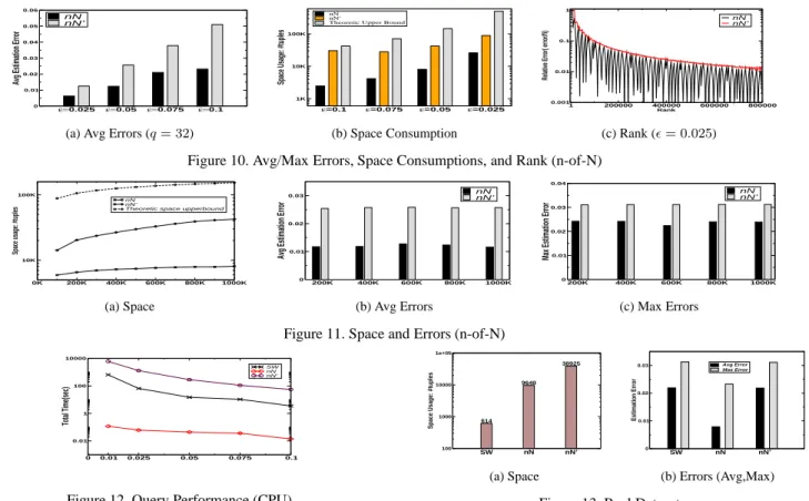
We repeated a similar set of tests, to evaluate nN and nN’, to those in Figure 6. The results are shown in Figure 10 for then-of-Nmodel, where we maken= 400KandN= 800K. We use the same data stream as in the experiments in Figure 6. The algorithm nN clearly outperforms nN’, as well as those worst-case based theoretical bounds.
We conducted another set of experiments to examine the impacts ofnandN on the algorithm nN and nN’. The data stream used is the same as above with1000Kelements. The experiment results are reported in Figure 11.
Figure 11 (a) shows the space consumptions for the al-gorithm nN whereN changes fromN = 100K toN = 1000K. Note that the theoretic space upper-bound means the one for the algorithm nN.
Figure 11 (b) and (c) show the average and maximum er-rors, respectively, whenN = 1000K, andnchanges from
614 9648
38925
SW nN nN’ 100
1000 10000 1e+05
Space Usage: #tuples
(a) Space
SW nN nN’ 0
0.01 0.02 0.03
Estimation Error
Avg Error Max Error
(b) Errors (Avg,Max)
Figure 13. Real Dataset
n = 200Kton = 1000K. For eachn, we run randomly 320queries.
6.3
Query Costs
In Figure 12, we show the total query processing costs (CPU) for running20Kqueries, where all the parameters take the default values and the number of the data stream elements is1000K.
Note that the algorithm nN Query is the most efficient one as there is no merge operation.
6.4
Real Dataset Testing
The topic detection and tracking (TDT) is an important issue in information retrieval and text mining (http:// www.ldc.upenn.edu/Projects/TDT3/). We have archived the news stories received through Reuters real-time datafeed, which contains 365,288 news stories and 100,672,866 (duplicate) words. All articles such as “the” and “a” are removed before term stemming.
We use N = 800K and = 0.05. Figure 13 shows space consumptions and average/max errors usingq = 32, for SW, nN and nN’. They follow similar trends to those for synthetic data.
In summary, our experiment results demonstrated that the algorithm SW and the algorithm nN perform much bet-ter than their worst case based theoretical bounds, respec-tively. In addition to good theoretical bounds, the algorithm SW and the algorithm nN also outperform the other tech-niques.
Table 2. Comparing Our Results with Recent Results in Quantile Computation
Authors Year Computation Model Precision Space Requirement
Alsabti, et. al. [2] 1997 data sequence N, deterministic Ω(
N )
Manku, et. al. [17] 1998 data sequence N, deterministic O(log2(N))
Manku, et. al. [18] 1999 data stream/appending only N, conf =1−δ O(−1log2−1+−1log2logδ−1) Greenwald and Khanna [10] 2001 data stream/appending only N, deterministic O(1log(N))
Gilbert et. al. [9] 2002 data stream/with deletion N, conf =1−δ O((log2|U|log log(|U|/δ))/2) Lin, et. al. [this paper] 2003 data stream/sliding window N, deterministic O(log(2N) +12)
Lin, et. al. [this paper] 2003 data stream/n-of-N N, deterministic O(log2(2N))
7
Conclusions
In this paper, we presented our results on maintaining quantile summaries for data streams. While there is quite a lot of related work reported in the literature, the work re-ported here is among the first attempts to develop space effi-cient, one pass, deterministic quantile summary algorithms with performance guarantees under the sliding window model of data streams. Furthermore, we extended the slid-ing window model to propose a newn-of-Nmodel which we believe has wide applications. As our performance study indicated, the algorithms proposed for both models provide much more accurate quantile estimates than the guaranteed precision while requiring much smaller space than the worst case bounds.
In Table 2, we compare our results with the recent results in quantile computation under various models.
An immediate future work is to investigate the prob-lem of maintaining other statistics under our newn-of-N model. Furthermore, the technique developed in this work that merges multiple-approximate quantile sketches into a single-approximate quantile sketches is expected to have applications in distributed and parallel systems. One possi-ble work is to investigate the issues related to maintain dis-tributed quantile summaries for large systems for a sliding window.
References
[1] R. Agrawal and A. Swami. A one-pass space-efficient algo-rithm for finding quantiles. In S. Chaudhuri, A. Deshpande, and R. Krishnamurthy, editors, COMAD, 1995.
[2] K. Alsabti, S. Ranka, and V. Singh. A one-pass algorithm for accurately estimating quantiles for disk-resident data. In The VLDB Journal, pages 346–355, 1997.
[3] Y. Chen, G. Dong, J. Han, B. W. Wah, and J. Wang. Multi-dimensional regression analysis of time-series data streams. In VLDB, 2002.
[4] A. Das, J. Gehrke, and M. Riedewald. Approximate join processing over data streams. In SIGMOD, 2003.
[5] M. Datar, A. Gionis, P. Indyk, and R. Motwani. Maintaining stream statistics over sliding windows: (extended abstract). In ACM-SIAM, pages 635–644, 2002.
[6] A. Dobra, M. N. Garofalakis, J. Gehrke, and R. Rastogi. Processing complex aggregate queries over data streams. In SIGMOD, 2002.
[7] M. Garofalakis and A. Kumar. Correlating xml data streams using tree-edit distance embeddings. In SIGMOD-SIGACT-SIGART, 2003.
[8] J. Gehrke, F. Korn, and D. Srivastava. On computing corre-lated aggregates over continual data streams. In SIGMOD, pages 13–24, 2001.
[9] A. C. Gilbert, Y. Kotidis, S. Muthukrishnan, and M. J. Strauss. How to summarize the universe: Dynamic main-tenance of quantiles. In VLDB, 2002.
[10] M. Greenwald and S. Khanna. Space-efficient online com-putation of quantile summaries. In SIGMOD, pages 58–66, 2001.
[11] S. Guha and N. Koudas. Approximating a data stream for querying and estimation: Algorithms and performance eval-uation. In ICDE, 2002.
[12] S. Guha, N. Koudas, and K. Shim. Data-streams and his-tograms. In STOC, pages 471–475, 2001.
[13] S. Guha, N. Mishra, R. Motwani, and L. O’Callaghan. Clus-tering data streams. In FOCS, pages 359–366, 2000. [14] A. Gupta and D. Suciu. Stream processing of xpath queries
with predicates. In SIGMOD, 2003.
[15] J. Kang, J. Naughton, and S. Viglas. Evaluation window joins over undounded streams. In ICDE, 2003.
[16] G. Manku and R. Motwani. Approximate frequency counts over data streams. In VLDB, 2002.
[17] G. S. Manku, S. Rajagopalan, and B. G. Lindsay. Approxi-mate medians and other quantiles in one pass and with lim-ited memory. In SIGMOD, pages 426–435, 1998.
[18] G. S. Manku, S. Rajagopalan, and B. G. Lindsay. Random sampling techniques for space efficient online computation of order statistics of large datasets. In SIGMOD, pages 251– 262, 1999.
[19] J. Munro and M. Paterson. Selection and sorting wiith lim-ited storage. In TCS12, 1980.
[20] C. Olston, J. Jiang, and J. Widom. Adaptive filters for con-tinuous queries over distributed data streams. In SIGMOD, 2003.
[21] R. Ramakrishan. Database Management Systems. McGraw-Hill, 2002.
[22] Y. Zhu and D. Shasha. Statstream:statistical monitoring of thousands of data streams in real time. In VLDB, 2002.