Expander Flows, Geometric Embeddings and Graph Partitioning
SANJEEV ARORA Princeton University SATISH RAO and
UMESH VAZIRANI UC Berkeley
We give aO(√logn)-approximation algorithm for thesparsest cut,edge expansion,balanced separator, andgraph conductanceproblems. This improves the O(logn)-approximation of Leighton and Rao (1988). We use a well-known semidefinite relaxation with triangle inequality constraints. Central to our analysis is a geometric theorem about projections of point sets in�d,
whose proof makes essential use of a phenomenon called measure concentration.
We also describe an interesting and natural “approximate certificate” for a graph’s expansion, which involves embedding ann-node expander in it with appropriate dilation and congestion. We call this an expander flow.
Categories and Subject Descriptors: F.2.2 [Theory of Computation]: Analysis of Algorithms and Problem Complexity; G.2.2 [Mathematics of Computing]: Discrete Mathematics and Graph Algorithms
General Terms: Algorithms,Theory
Additional Key Words and Phrases: Graph Partitioning,semidefinite programs,graph separa-tors,multicommodity flows,expansion,expanders
1. INTRODUCTION
Partitioning a graph into two (or more) large pieces while minimizing the size of the “interface” between them is a fundamental combinatorial problem. Graph partitions or separators are central objects of study in the theory of Markov chains, geometric embeddings and are a natural algorithmic primitive in numerous settings, including clustering, divide and conquer approaches, PRAM emulation, VLSI layout, and packet routing in distributed networks. Since finding optimal separators is NP-hard, one is forced to settle for approximation algorithms (see Shmoys [1995]). Here we give new approximation algorithms for some of the important problems in this class.
Graph partitioning involves finding a cut with few crossing edges conditioned on or normalized by the size of the smaller side of the cut. The problem can be made precise in different ways, giving rise to several related measures of the quality of the cut, depending on precisely how size is measured, such as conductance, expansion, normalized or sparsest cut. Precise definitions appear in Section 2. These measures are approximation reducible within a constact factor (Leighton and Rao [1999]), are allNP-hard, and arise naturally in different contexts.
A weak approximation for graph conductance follows from the connection —first discovered in the Author’s address: S. Arora, Computer Science Department, Princeton University. www.cs.princeton.edu/∼arora. Work done partly while visiting UC Berkeley (2001-2002) and the Institute for Advanced Study (2002-2003). Supported by David and Lucille Packard Fellowship, and NSF Grants CCR-0098180 and CCR-0205594 MSPA-MCS 0528414, CCF 0514993, ITR 0205594, NSF CCF 0832797.
S. Rao Computer Science Division, UC Berkeley. www.cs.berkeley.edu/∼satishr. Partially supported by NSF award CCR-0105533, CCF-0515304, CCF-0635357.
U. Vazirani. Computer Science Division, UC Berkeley.www.cs.berkeley.edu/∼vaziraniPartially supported by NSF ITR Grant CCR-0121555.
A preliminary version of this paper appeared at ACM Symposium on Theory of Computing, 2004
Permission to make digital/hard copy of all or part of this material without fee for personal or classroom use provided that the copies are not made or distributed for profit or commercial advantage, the ACM copyright/server notice, the title of the publication, and its date appear, and notice is given that copying is by permission of the ACM, Inc. To copy otherwise, to republish, to post on servers, or to redistribute to lists requires prior specific permission and/or a fee.
c
�20YY ACM 0004-5411/20YY/0100-0111 $5.00
context of Riemannian manifolds (Cheeger [1970])—between conductance and the eigenvalue gap of the Laplacian: 2Φ(G)≥λ≥Φ(G)2/2 (Alon and Milman [1985; Alon [1986; Jerrum and Sinclair [1989]). The
approximation factor is 1/Φ(G), and hence Ω(n) in the worst case, and O(1) only if Φ(G) is a constant. This connection between eigenvalues and expansion has had enormous influence in a variety of fields (see e.g. Chung [1997]).
Leighton and Rao [1999] designed the first true approximation by giving O(logn)-approximations for
sparsest cutandgraph conductance andO(logn)-pseudo-approximations1 forc-balanced
separa-tor. They used a linear programming relaxation of the problem based on multicommodity flow proposed
in Shahrokhi and Matula [1990]. These ideas led to approximation algorithms for numerous otherNP-hard problems, see Shmoys [1995]. We note that the integrality gap of the LP is Ω(logn), and therefore improving the approximation factor necessitates new techniques.
In this paper, we giveO(√logn)-approximations forsparsest cut,edge expansion, andgraph con-ductance and O(√logn)-pseudo-approximation toc-balanced separator. As we describe below, our
techniques have also led to new approximation algorithms for several other problems, as well as a break-through in geometric embeddings.
The key idea underlying algorithms for graph partitioning is to spread out the vertices in some abstract space while not stretching the edges too much. Finding a good graph partition is then accomplished by partitioning this abstract space. In the eigenvalue approach, the vertices are mapped to points on the real line such that the average squared distance is constant, while the average squared distance between the endpoints of edges is minimized. Intuitively, snipping this line at a random point should cut few edges, thus yielding a good cut. In the linear programming approach, lengths are assigned to edges such that the average distance between pairs of vertices is fixed, while the average edge length is small. In this case, it can be shown that a ball whose radius is drawn from a particular distribution defines a relatively balanced cut with few expected crossing edges, thus yielding a sparse cut.
Note that by definition, the distances in the linear programming approach form a metric (i.e., satisfy the triangle inequality) while in the eigenvalue approach they don’t. On the other hand, the latter approach works with a geometric embedding of the graph, whereas there isn’t such an underlying geometry in the former.
In this paper, we work with an approach that combines both geometry and the metric condition. Consider mapping the vertices to points on the unit sphere in�n such that the squared distances form a metric. We refer to this as an�2
2-representationof the graph. We say that it iswell-spreadif the average squared distance
among all vertex pairs is a fixed constant, sayρ. Define thevalueof such a representation to be the sum of squared distances between endpoints of edges. The value of thebest representation is (up to a factor 4) a lower bound on the capacity of the bestc-balanced separator, where 4c(1−c) =ρ. The reason is that every c-balanced cut in the graph corresponds to a�2
2representation in a natural way: map each side of the cut to
one of two antipodal points. The value of such a representation is clearly 4 times the cut capacity since the only edges that contribute to the value are those that cross the cut, and each of them contributes 4. The average squared distance among pairs of vertices is at least 4c(1−c).
Our approach starts by finding a well-spread representation of minimum value, which is possible in polyno-mial time using semidefinite programming. Of course, this minimum value representation will not in general correspond to a cut. The crux of this paper is to extract a low-capacity balanced cut from this embedding.
The key to this is a new result (Theorem 1) about the geometric structure of well-spread�2
2-representations:
they contain Ω(n) sized setsS andT that are well-separated, in the sense that every pair of pointsvi∈S andvj ∈T must be at least ∆ = Ω(1/√logn) apart in�2
2 (squared Euclidean) distance. The setS can be
used to find a good cut as follows: consider all points within some distance δ ∈ [0,∆] from S, where δ is chosen uniformly at random. The quality of this cut depends upon the value of representation. In particular, if we start with a representation of minimum value, the expected number of edges crossing such a cut must be small, since the length of a typical edge is short relative to ∆.
1For any fixedc�< cthe pseudo-approximation algorithm finds ac�-balanced cut whose expansion is at mostO(logn) times
expansion of the bestc-balanced cut.
Furthermore, the sets S andT can be constructed algorithmically by projecting the points on a random line as follows (Section 3): for suitable constant c, the leftmostcn and rightmost cn points on the line are our first candidates for S andT. However, they can contain pairs of points vi ∈S, vj ∈T whose squared distance is less than ∆, which we discard. The technically hard part in the analysis is to prove that not too many points get discarded. This delicate argument makes essential use of a phenomenon calledmeasure concentration, a cornerstone of modern convex geometry (see Ball [1997]).
The result on well-separated sets is tight for ann-vertex hypercube —specifically, its natural embedding on the unit sphere in�lognwhich defines an �2
2metric— where measure concentration implies that any two
large sets are within O(1/√logn) distance. The hypercube example appears to be a serious obstacle to improving the approximation factor for finding sparse cuts, since the optimal cuts of this graph (namely, the dimension cuts) elude all our rounding techniques. In fact, hypercube-like examples have been used to show that this particular SDP approach has an integrality gap of Ω(log logn) (Devanur et al. [2006; Krauthgamer and Rabani [2006]).
Can our approximation ratio be improved over O(√logn)? In Section 8 we formulate a sequence of conditions that would imply improved approximations. Our theorem on well-separated sets is also important in study of metric embeddings, which is further discussed below.
1.0.0.1 Expander flows:. While SDPs can be solved in polynomial time, the running times in practice are not very good. Ideally, one desires a faster algorithm, preferably one using simple primitives like shortest paths or single commodity flow. In this paper, we initiate such a combinatorial approach that realizes the same approximation bounds as our SDP-based algorithms, but does not use SDPs. Though the resulting running times in this paper are actually inferior to the SDP-based approach, subsequent work has led to algorithms that are significantly faster than the SDP-based approach.
We design our combinatorial algorithm using the notion ofexpander flows, which constitute an interesting and natural “certificate” of a graph’s expansion. Note that any algorithm that approximates edge expansion α = α(G) must implicitly certify that every cut has large expansion. One way to do this certification is to embed2 a complete graph into the given graph with minimum congestion, say µ. (Determining µ
is a polynomial-time computation using linear programming.) Then it follows that every cut must have expansion at least n/µ. (See Section 7.) This is exactly the certificate used in the Leighton-Rao paper, where it is shown that congestion O(nlogn/α(G)) suffices (and this amount of congestion is required on some worst-case graphs). Thus embedding the complete graph suffices to certify that the expansion is at leastα(G)/logn.
Our certificate can be seen as a generalization of this approach, whereby we embed not the complete graph but some flow that is an “expander” (a graph whose edge expansion is Ω(1)). We show that for every graph there is an expander flow that certifies an expansion of Ω(α(G)/√logn) (see Section 7). This near-optimal embedding of an expander inside an arbitrary graph may be viewed as a purely structural result in graph theory. It is therefore interesting that this graph-theoretic result is proved using geometric arguments similar to the ones used to analyse our SDP-based algorithm. (There is a natural connection between the two algorithms since expander flows can be viewed as a natural family of dual solutions to the above-mentioned SDP, see Section 7.4.) In fact, the expander flows approach was the original starting point of our work.
How does one efficiently compute an expander flow? The condition that the multicommodity flow is an expander can be imposed by exponentially many linear constraints. For each cut, we have a constraint stating that the amount of flow across that cut is proportional to the number of vertices on the smaller side of the cut. We use the Ellipsoid method to find the feasible flow. At each step we have to check if any of these exponentially many constraints are violated. Using the fact that the eigenvalue approach gives a constant factor approximation when the edge expansion is large, we can efficiently find violated constraints (to within constant approximation), and thus find an approximately feasible flow in polynomial time using
2Note that this notion of graph embedding has no connection in general to geometric embeddings of metric spaces, or geometric embeddings of graphs using semidefinite programming. It is somewhat confusing that all these notions of embeddings end up being relevant in this paper.
the Ellipsoid method. Arora, Hazan, and Kale [2004] used this framework to design an efficient ˜O(n2) time
approximation algorithm, thus matching the running time of the best implementations of the Leighton-Rao algorithm. Their algorithm may be thought of as a primal-dual algorithm and proceeds by alternately computing eigenvalues and solving min-cost multicommodity flows. Khandekar, Rao, and Vazirani [2006] use the expander flow approach to break the ˜O(n2) multicommodity flow barrier and rigorously analyse
an algorithm that resembles some practially effective heuristics (Lang and Rao [2004]). The analysis gives a worse O(log2n) approximation for sparsest cut but requires only O(log2n) invocations of a single
commodity maximum flow algorithm. Arora and Kale [2007] have improved this approximation factor to O(logn) with a different algorithm. Thus one has the counterintuitive result that an SDP-inspired algorithm runs faster than the older LP-inspired algorithm a la Leighton-Rao, while attaining the same approximation ratio. Arora and Kale also initiate a new primal-dual and combinatorial approach to other SDP-based approximation algorithms.
Related prior and subsequent work.
Semidefinite programming and approximation algorithms: Semidefinite programs (SDPs) have nu-merous applications in optimization. They are solvable in polynomial time via the ellipsoid method (Gr¨otschel et al. [1993]), and more efficient interior point methods are now known (Alizadeh [1995; Nesterov and Ne-mirovskii [1994]). In a seminal paper, Goemans and Williamson [1995] used SDPs to design good approx-imation algorithms for MAX-CUT and MAX-k-SAT. Researchers soon extended their techniques to other problems (Karger et al. [1998; Karloff and Zwick [1997; Goemans [1998]), but lately progress in this direction had stalled. Especially in the context of minimization problems, the GW approach of analysing “random hyperplane” rounding in an edge-by-edge fashion runs into well-known problems. By contrast, our theorem about well separated sets in �2
2 spaces (and the “rounding” technique that follows from it) takes a more
global view of the metric space. It is the mathematical heart of our technique, just as the region-growing argument was the heart of the Leighton-Rao technique for analysing LPs.
Several papers have pushed this technique further, and developed closer analogs of the region-growing argument for SDPs using our main theorem. Using this they design new √logn-approximation algorithms for graph deletion problems such as2cnf-deletionandmin-uncut(Agarwal et al. [2005]), formin-linear arrangement(Charikar et al. [2006; Feige and Lee [2007]), andvertex separators(Feige et al. [2005a]).
Similarly,min-vertex covercan now be approximated upto a factor 2−Ω(1/√logn) (Karakostas [2005]), an improvement over 2−Ω(log logn/logn) achieved by prior algorithms. Also, aO(√logn) approximation algorithm for node cuts is given in Feige et al. [2005b].
However, we note that the Structure Theorem does not provide a blanket improvement for all the problems for which O(logn) algorithms were earlier designed using the Leighton-Rao technique. In particular, the integrality gap of the SDP relaxation for min-multicutwas shown to be Ω(logn) (Agarwal et al. [2005]),
the same (upto a constant factor) as the integrality gap for the LP relaxation.
Analysis of random walks: The mixing time of a random walk on a graph is related to the first nonzero eigenvalue of the Laplacian, and hence to the edge expansion. Of various techniques known for upper bounding the mixing time, most rely on lower bounding the conductance. Diaconis and Saloff-Coste [1993] describe a very general idea called the comparison technique, whereby the edge expansion of a graph is lower bounded by embedding aknowngraph withknownedge expansion into it. (The embedding need not be efficiently constructible; existence suffices.) Sinclair [1992] suggested a similar technique and also noted that the Leighton-Rao multicommodity flow can be viewed as a generalization of the Jerrum-Sinclair [1989] canonical path argument. Our results on expander flows imply that the comparison technique can be used to always get to withinO(√logn) of the correct value of edge expansion.
Metric spaces and relaxations of the cut cone: The graph partitioning problem is closely related to geometric embeddings of metric spaces, as first pointed out by Linial, London and Rabinovich [1995] and Aumann and Rabani [1998]. Thecut coneis the cone of all cut semi-metrics, and is equivalent to the cone of all�1semi-metrics. Graph separation problems can often be viewed as the optimization of a linear function
over the cut cone (possibly with some additional constraints imposed). Thus optimization over the cut
cone isNP-hard. However, one could relax the problem and optimize over some other metric space, embed this metric space in �1 (hopefully, with low distortion), and then derive an approximation algorithm. This
approach is surveyed in Shmoys’s survey [1995]. The integrality gap of the obvious generalization of our SDP fornonuniform sparsest cut is exactly the same as as the worst-case distortion incurred in embedding
n-point�2
2metrics into�1. A famous result of Bourgain shows that the distortion is at mostO(logn), which
yields an O(logn)-approximation fornonuniform sparsest cut. Improving this has been a major open
problem.
The above connection shows that anα(n) approximation for conductance and other measures for graph partitioning would follow from any general upper bound α(n) for the minimum distortion for embedding �2
2 metrics into �1. Our result on well separated sets has recently been used Arora et al. [2008] to bound
this distortion byO(√lognlog logn), improving on Bourgain’s classicalO(logn) bound that applies to any metric. In fact, they give a stronger result: an embedding of �2
2 metrics into �2. Since any �2 metric is an
�1 metric, which in turn is an�22metric, this also gives an embedding of�1into�2with the same distortion.
This almost resolves a central problem in the area of metric embeddings, since any �2 embedding of the
hypercube, regarded as an�1 metric, must suffer an Ω(√logn) distortion (Enflo [1969]).
A key idea in these new developments is our above-mentioned main theorem about the existence of well-separated setsS, T in well-spread�2
2metrics. This can be viewed as a weak “average case” embedding from
�2
2into�1 whose distortion isO(√logn). This is pointed out by Chawla, Gupta, and R¨acke [2005], who used
it together with the measured descent technique of Krauthgamer, Lee, Mendel, Naor [2005] to show that n-point�2
2metrics embed into�2(and hence into�1) with distortionO(log3/4n). Arora, Lee, and Naor [2008]
improved this distortion toO(√lognlog logn), which is optimal up to log lognfactor.
To see why our main theorem is relevant in embeddings, realize that usually the challenge in producing such an embedding is to ensure that the images of any two points from the original�2
2metric are far enough
apart in the resulting�1 metric. This is accomplished in Arora et al. [2008] by considering dividing possible
distances into geometrically increasing intervals and generating coordinates at each distance scale. Our main theorem is used to find a well-separated pair of sets, S and T, for each scale, and then to use “distance to S” as the value of the corresponding coordinate. Since each node in T is at least ∆/√logn away from every node in S, this ensures that a large number of ∆-separated pairs of nodes are far enough apart. The O(√lognlog logn) bound on the distortion requires a clever accounting scheme across distance scales.
We note that above developments showed that the integrality gap for nonuniform sparsest cut is
O(√lognlog logn). There was speculation that the integrality gap may even be O(1), but Khot and Vish-noi [2005] have shown it is at least (log logn)� for some� >0.
2. DEFINITIONS AND RESULTS
We first define the problems considered in this paper; all are easily proved to be NP-hard (Leighton and Rao [1999]). Given a graph G= (V, E), the goal in the uniform sparsest cut problem is to determine
the cut (S, S) (where|S| ≤��S��without loss of generality) that minimizes
�
�E(S, S)��
|S|��S�� . (1)
Since |V|/2 ≤ ��S�� ≤ |V|, up to a factor 2 computing the sparsest cut is the same as computing the edge expansion of the graph, namely,
α(G) = min
S⊆V,|S|≤|V|/2
�
�E(S, S)��
|S| .
Since factors of 2 are inconsequential in this paper, we use the two problems interchangeably. Furthermore, we often shortenuniform sparsest cutto justsparsest cut. In another related problem,c -balanced-separator, the goal is to determine αc(G), the minimum edge expansion among all c-balanced cuts. (A
cut (S, S) isc-balancedif both S, S have at least c|V| vertices.) In thegraph conductanceproblem we
wish to determine
Φ(G) = min
S⊆V,|E(S)|≤|E|/2
�
�E(S, S)��
|E(S)| , (2)
where E(S) denotes the multiset of edges incident to nodes inS (i.e., edges with both endpoints inS are included twice).
There are well-known interreducibilities among these problems for approximation. The edge expansion, α, of a graph is betweenn/2 and ntimes the optimal sparse cut value. The conductance problem can be reduced to the sparsest cut problem by replacing each node with a degree dwith a clique on dnodes; any sparse cut in the transformed graph does not split cliques, and the sparsity of any cut (that does not split cliques) in the transformed graph is within a constant factor of the conductance of the cut. The sparsest cut problem can be reduced to the conductance problem by replacing each node with a large (say sizedC=n2
size) clique. Again, small cuts don’t split cliques and a (clique non-splitting) cut of conductance Φ in the transformed graph corresponds to the a cut in the original of sparsity Φ/C2. The reductions can be bounded
degree as well (Leighton and Rao [1999]).
As mentioned, all our algorithms depend upon a geometric representation of the graph.
Definition 1 (�2
2-representation) An �22-representationof a graph is an assignment of a point (vector)
to each node, say vi assigned to nodei, such that for all i, j, k:
|vi−vj|2+|vj−vk|2≥ |vi−vk|2 (triangle inequality) (3) An�2
2-representation is called aunit-�22 representationif all points lie on the unit sphere (or equivalently, all
vectors have unit length.)
Remark 1 We mention two alternative descriptions of unit�2
2-representations which however will not play
an explicit role in this paper. (i) Geometrically speaking, the above triangle inequality says that everyviand vksubtend a nonobtuse angle atvj. (ii) Every positive semidefiniten×nmatrix has aCholesky factorization, namely, a set ofnvectorsv1, v2, . . . , vn such thatMij =�vi, vj�. Thus a unit-�22-representation for annnode
graph can be alternatively viewed as a positive semidefinite n×n matrixM whose diagonal entries are 1 and∀i, j, k, Mij+Mjk−Mik≤1.
We note that an�2
2-representation of a graph defines a so-called�22 metric on the vertices, whered(i, j) =
|vi−vj|2.We’ll now see how the geometry of�2
2 relates to the properties of cuts in a graph.
Every cut (S, S) gives rise to a natural unit-�2
2-representation, namely, one that assigns some unit vector
v0 to every vertex inS and−v0 to every vertex inS.
Thus the following SDP is a relaxation forαc(G) (scaled by cn).
min 1
4
�
{i,j}∈E
|vi−vj|2 (4)
∀i |vi|2= 1 (5)
∀i, j, k |vi−vj|2+|vj−vk|2≥ |vi−vk|2 (6)
�
i<j
|vi−vj|2≥4c(1−c)n2 (7)
This SDP motivates the following definition.
Definition 2 An �2
2-representation isc-spread if equation (7) holds. Journal of the ACM, Vol. V, No. N, Month 20YY.
Similarly the following is a relaxation forsparsest cut(up to scaling byn; see Section 6).
min �
{i,j}∈E
|vi−vj|2 (8)
∀i, j, k |vi−vj|2+|vj−vk|2≥ |vi−vk|2 (9)
�
i<j
|vi−vj|2= 1 (10)
As we mentioned before the SDPs subsume both the eigenvalue approach and the Leighton-Rao ap-proach (Goemans [1998]). We show that the optimum value of thesparsest cutSDP is Ω(α(G)n/√logn),
which shows that the integrality gap isO(√logn). 2.1 Main theorem about�2
2-representations
In general,�2
2-representations are not well-understood3. This is not surprising since in�dthe representation
can have at most 2d distinct vectors (Danzer and Branko [1962]), so our three-dimensional intuition is of limited use for graphs with more than 23 vertices. The technical core of our paper is a new theorem about
unit�22-representations.
Definition 3 (∆-separated) If v1, v2, . . . , vn ∈ �d, and ∆ ≥ 0, two disjoint sets of vectors S, T are
∆-separatedif for everyvi∈S, vj∈T,|vi−vj|2≥∆.
Theorem 1 (Main)
For everyc >0, there arec�, b >0such that everyc-spread unit-�2
2-representation withnpoints contains
∆-separated subsetsS, T of sizec�n, where∆ =b/√logn. Furthermore, there is a randomized polynomial-time algorithm for finding these subsetsS, T.
Remark 2 The value of ∆ in this theorem is best possible up to a constant factor, as demonstrated by
the natural embedding (scaled to give unit vectors) of the boolean hypercube{−1,1}d. These vectors form a unit �2
2-representation, and the isoperimetric inequality for hypercubes shows that every two subsets of
Ω(n) vectors contain a pair of vectors — one from each subset — whose squared distance isO(1/√logn) (here n = 2d). Theorem 1 may thus be viewed as saying that every Ω(1)-spread unit �2
2-representation is
“hypercube-like” with respect to the property mentioned in the theorem. Some may view this as evidence for the conjecture that �2
2-representations are indeed like hypercubes (in particular, embed in�1 with low
distortion). The recent results in (Chawla et al. [2005; Arora et al. [2008]), which were inspired by our paper, provide partial evidence for this belief.
2.1.1 Corollary to Main Theorem: √logn-approximation. LetW =�{i,j}∈E1
4|vi−vj|
2be the optimum
value for the SDP defined by equations (4)–(7). Since the vectorsvi’s obtained from solving the SDP satisfy the hypothesis of Theorem 1, as an immediate corollary to the theorem we show how to produce ac�-balanced cut of sizeO(W√logn). This uses the region-growing argument of Leighton-Rao.
Corollary 2
There is a randomized polynomial-time algorithm that finds with high probability a cut that isc�-balanced, and has sizeO(W√logn).
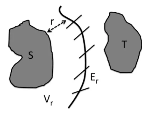
Proof: We use the algorithm of Theorem 1 to produce ∆-separated subsetsS, T for ∆ =b/√logn. LetV0
denote the vertices whose vectors are in S. Associate with each edgee={i, j} a lengthwe= 14|vi−vj|2.
(ThusW =�e∈Ewe.)SandT are at least ∆ apart with respect to this distance. LetVsdenote all vertices within distance sof S. Now we produce a cut as follows: pick a random numberr between 0 and ∆, and output the cut (Vr, V −Vr). SinceS⊆Vr andT ⊆V \Vr, this is ac�-balanced cut.
To bound the size of the cut, we denote by Er the set of edges leaving Vr. Each edge e = {i, j} only contributes toErforrin the open interval (r1, r2),wherer1=d(i, V0) andr2=d(j, V0). Triangle inequality
3As mentioned in the introduction, it has been conjectured that they are closely related to the better-understood�1 metrics.
Fig. 1. Vr is the set of nodes whose distance on the weighted graph toSis at mostr. Set of edges leaving this set isEr. implies that|r2−r1| ≤we. Hence
W =�
e we≥
� ∆
s=0|
Es|.
Thus, the expected value of |Er| over the interval [0,∆] is at mostW/∆.The algorithm thus produces a cut of size at most 2W/∆ =O(W√logn) with probability at least 1/2.
✷
3.
∆ = Ω(LOG
−2/3N
)-SEPARATED SETS
We now describe an algorithm that given a c-spread �2
2 representation finds ∆-separated sets of size Ω(n)
for ∆ = Θ(1/log2/3n). Our correctness proof assumes a key lemma (Lemma 7) whose proof appears in
Section 4. The algorithm will be improved in Section 5 to allow ∆ = Θ(1/√logn). The algorithm, set-find, is given ac-spread �2
2-representation. Constantsc�, σ >0 are chosen
appropri-ately depending onc.
set-find:
Input: Ac-spread unit-�2
2 representationv1, v2, . . . , vn ∈ �d.
Parameters: Desired separation ∆, desired balancec�, and projection gap,σ.
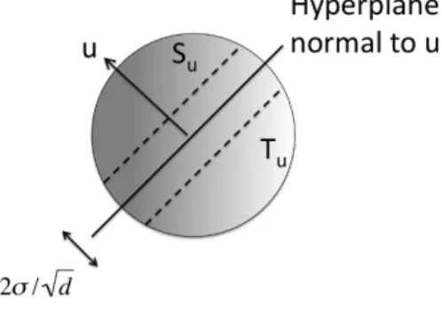
Step 1: Project the points on a uniformly random lineupassing through the origin, and compute the largest valuemwhere half the pointsv, have�v, u� ≥m.
Then, we specify that
Su={vi:�vi, u� ≥m+√σ d}, Tu={vi:�vi, u� ≤m}. If|Su|<2c�n, HALT.a
Step 2: Pick anyvi ∈Su, vj ∈Tu such that|vi−vj|2≤∆, and deletevi from Su and vj from Tu. Repeat until no suchvi, vj can be found and output the remaining setsS, T.
aWe note that we could have simply chosen m to be 0 rather than to be the median, but this version of the
procedure also applies for finding sparsest cuts.
Remark 3 The procedure set-find can be seen as a rounding procedure of sorts. It starts with a “fat”
random hyperplane cut (cf. Goemans-Williamson [1995]) to identify the setsSu, Tu of vertices that project far apart. It then prunes these sets to find setsS, T.
Fig. 2. The setsSuandTufound duringset-find. The figure assumesm= 0.
Notice that ifset-finddoes notHALTprematurely, it returns a ∆-separated pair of sets. It is easy to
show that the likelihood of premature halting is small, and we defer it to the next subsection. The main challenge is to show that that the ∆-separated sets are large, i.e., that no more thanc�npairs of points are deleted fromSu andTu. This occupies the bulk of the paper and we start by giving a very high level picture. 3.1 Broad Outline of Proof
First observe that the Theorem is almost trivial if we desire O(logn)-separated sets S and T (in other words,∆ = Ω(1/logn)). The reason is that the expected projection of a vector of length� is�/√dand the chance that it is k times larger is exp(−k2) (see Lemma 5). Since a pair is deleted only if the projection
of vi−vj onuexceeds Ω(1/√d), the chance that a pair satisfying |vi−vj|=O(1/√logn) or |vi−vj|2=
O(1/logn) is deleted is exp(−O(logn)), which is polynomially small. So with high probabilityno pair is deleted. Unfortunately, this reasoning breaks for the case of interest, namely ∆ = Ω(log−2/3n), when many
pairs may get deleted.
So assume the algorithm fails with high probability when ∆ = Ω(log−2/3n). We show that for most
directionsuthere is a sequence ofk= log1/3npointsv1, v2, . . . , vk such that every successive pair is close,
i.e. |vi−vi+1|2≤∆, and their difference has a large projection onu, i.e. �vi−vi+1, u� ≥2σ/√d. The main
point is that these projections all have the samesign, and thus adding them we obtain�v1−vk, u� ≥2σk/√d.
Thus the projection scales linearly ink whereas the Euclidean distance between the first and last point in the sequence scales as√k, since the points come from an�2
2metric. For the chosen values ofk,∆, this means
that Euclidean distance between the first and last point is O(1) whereas the projection is Ω(√logn/√d) —large enough that the probability that such a large projection exists foranyof the�n
2
�pairs iso(1). This
is a contradiction, allowing us to conclude that the algorithm did not fail with high probability (in other words, did manage to output large ∆-separated sets).
The idea in finding this sequence of points is to find them among deleted pairs (corresponding to different directions u). This uses the observation that the deleted pairs for a directionuform a matching, and that the path for a directionucan in fact use deleted pairs from a “nearby” directionu�; something that is made
formal using measure concentration. The argument uses induction, and actually shows the existence of many sequences of the type described above, not just one.
3.2 Covers and Matching Covers
Let us start by formalizing the condition that must hold if the algorithm fails with high probability, i.e., for most choices of directions u, Ω(n) pairs must be deleted. It is natural to think of the deleted pairs as forming a matching.
Definition 4 A (σ, δ, c�)-matching cover of a set of points in �d is a set M of matchings such that for at least a fractionδ of directions u, there exists a matching Mu ∈ Mof at leastc�n pairs of points, such that
each pair(vi, vj)∈Mu,satisfies
�vi−vj, u� ≥2σ/√d.
The associated matching graph M is defined as the multigraph consisting of the union of all matchings Mu.
In the next section, we will show that step 1 succeeds with probability δ. This implies that if with probability at leastδ/2 the algorithm didnotproduce sufficiently large ∆-separated pair of sets, then with probability at leastδ/2 many pairs were deleted. Thus the following lemma is straightforward.
Lemma 3
Ifset-findfails with probability greater than1−δ/2, on a unitc-spread�2
2-representation, then the set of
points has a(σ, δ/2, c�)-matching cover.
The definition of (σ, δ, c�)-matching coverMof a set of points suggests that for many directions there are
many disjoint pairs of points that have long projections. We will work with a related notion.
Definition 5 ((σ, δ)-uniform-matching-cover) A set of matchings M (σ, δ)-uniform-matching-covers
a set of points V ⊆ �d if for every unit vector u
∈ �d, there is a matching Mu of V such that every (vi, vj)∈Mu satisfies|�u, vi−vj�| ≥ √2σ
d, and for everyi,µ(u:vi matched in Mu)≥δ. We refer to the set of matchingsM to be thematching cover ofV.
Remark 4 The main difference from Definition 4 is that every point participates in Mu with constant probability for a random directionu,whereas in Definition 4 this probability could be even 0.
Lemma 4
If a set ofnvectors is(σ, γ, β)-matching covered byM, then they contain a subsetX ofΩ(nδ)vectors that are(σ, δ)-uniformly matching covered byM, where δ= Ω(γβ).
Proof: Consider the multigraph consisting of the union of all matchingsMu’s as described in Definition 4.
The average node is inMufor at leastγβmeasure of directions. Remove all nodes that are matched on fewer than γβ/2 measure of directions (and remove the corresponding matched edges from the Mu’s). Repeat. The aggregate measure of directions removed is at mostγβn/2. Thus at leastγβn/2 aggregate measure on directions remains. This implies that there are at least γβn/4 nodes left, each matched in at least γβ/4 measure of directions. This is the desired subsetX.
✷
To carry out our induction we need the following weaker notion of covering a set:
Definition 6 ((�, δ)-cover) A set{w1, w2, . . . ,} of vectors in �d is an (�, δ)-cover if every |wj| ≤1 and
for at least δ fraction of unit vectors u∈ �d, there exists a j such that
�u, wj� ≥ �. We refer toδ as the covering probabilityand� as theprojection lengthof the cover.
A pointv is(�, δ)-covered by a set of points X if the set of vectors{x−v|x∈X}is an (�, δ)-cover.
Remark 5 It is important to note that matching covers are substantially stronger notion than covers. For
example thed-dimensional hypercube √1
d{−1,1}
dis easily checked to be an (Ω(1),Ω(1))-cover (equivalently, the origin is (Ω(1),Ω(1)) covered), even though it is only (Θ(1),Θ(1/√d)) uniformly matching covered. This example shows how a single outlier in a given direction can cover all other points, but this is not sufficient for a matching cover.
3.3 Gaussian Behavior of Projections
Before we get to the main lemma and theorem, we introduce a basic fact about projections and use it to show that step 1 ofset-findsucceeds with good probability.
Lemma 5 (Gaussian behavior of projections)
Ifv is a vector of length�in�d anduis a randomly chosen unit vector then (1) forx≤1,Pr[|�v, u�| ≤√x�
d]≤3x.
(2) forx≤√d/4,Pr[|�v, u�| ≥√x� d]≤e
−x2/4.
Formally, to show that step 1 of set-findsucceeds with good probability, we prove that the point sets
satisfy conditions in the following definition.
Definition 7 A set ofn points{v1, . . . , vn} ∈ �d is (σ, γ, c�)-projection separated if for at least γ fraction
of the directionsu,|Su| ≥2c�n, where
Su={i:�vi, u� ≥m+σ/√d}, withm being the median value of{�vi, u�}.
Using part (i) of Lemma 5, we show that the points are sufficiently projection separated. Here, it is convenient for the points to be on the surface of the unit sphere. Later, for approximating sparsest cut
we prove a similar statement without this condition.
Lemma 6
For every positivec <1/3, there arec�, σ, δ >0, such that everyc-spread unit�2
2-representation is(σ, δ, c�
)-projection separated.
Proof:Thec-spread condition states that�k,j|vk−vj|2≥4c(1−c)n2.Since
|vk−vj| ≤2, we can conclude that �k,j|vk−vj| ≥2c(1−c)n2. Applying Markov’s inequality, we can conclude that
|vi−vj| ≥c(1−c) for at leastc(1−c)n2 pairs.
For these pairsi, j, condition (1) of Lemma 5 implies that for a randomu, that|�vi, u� − �vj, u�|is at least c(1−c)/(9√d) with probability at least 1/3.
This implies that forσ=c(1−c)/18, the expected number of pairs where |�vi, u� − �vj, u�| ≥2σ/√dis at least (2/3)c(1−c)n2.Each such pair must have at least one endpoint whose projection is at leastσ/√d
away fromm; and each point can participate in at mostn such pairs. Therefore the expected number of points projected at leastσ/√daway frommis at least (2/3)c(1−c)n.
Applying Markov’s bound (and observing that the number of points is at most n) it follows that with probability at least (1/3)c(1−c) at least (1/3)c(1−c)npoints are projected at leastσ/√d away from m. By symmetry, half the time a majority of these points are in Su. Thus the lemma follows with δ =c� =
(1/6)c(1−c). c�= (1/6)c(1−c).
✷
3.4 Main Lemma and Theorem
We are now ready to formally state a lemma about the existence, for most directions, of many pairs of points whose difference vi−vj has a large projection on this direction. (Sometimes we will say more briefly that the “pair has large projection.”) For eachk, we inductively ensure that there is a large set of points which participate as one endpoint of such a (large projection) pair for at least half the directions. This lemma (and its variants) is a central technical contribution of this paper.
Definition 8 Given a set of n points that is (σ, δ, c�)-matching covered by M with associated matching
graph M, we define v to be in the k-core, Sk, if v is (k2√σ
d,1/2)-covered by points which are within k hops of v in the matching graphM.
Lemma 7
For every set of n points {v1, . . . , vn} that is (σ, δ, c�)-matching covered by M with associated matching
graphM, there are positive constantsa=a(δ, c�)andb=b(δ, c�)such that for every k≥1:
(1) Either|Sk| ≥akn.
(2) Or there is a pair(vi, vj)with distance at mostkin the matching graphM, such that
|vi−vj| ≥bσ/√k.
We use this lemma below to show thatset-findfinds Ω(1/log1/3n)-separated sets. Later, we develop a
modified algorithm for finding Ω(1/√logn)-separated sets.
Subsequently, the aforementioned paper by J. R. Lee [2005] strengthened case 1 of the lemma to show the existence ofSk of size at least|M|/2, and thus that case 2 meets the stronger condition that|vi−vj| ≥gσ for some constantg. This implies thatset-findwithout any modification finds large Ω(1/√logn)-separated
sets.
We can now prove the following theorem.
Theorem 8
Set-find finds an∆-separated set for ac-spread unit�2
2-representation{v1, . . . , vn}with constant probability
for some∆ = Ω(1/log2/3n).
Proof: Recall, that, by Lemma 3, if set-find fails, then the set of points is (σ, δ, c�)-matching covered.
Moreover, each pair (vi, vj) in any matchingMu for a directionusatisfies|vi−vj| ≤√∆ and�vi−vj, u� ≥ 2σ/√d.
We will now apply Lemma 7 to show that such a matching covered set does not exist for ∆ = Θ(1/log2/3n),
which means that set-find cannot fail for this ∆. Concretely, we show that neither case of the Lemma
holds fork=bσ/√∆ whereb is the constant defined in the Lemma. Let us start by dispensing with Case 2. Since the metric is�2
2, a pair of points (vi, vj) within distancekin
the matching graph satisfies|vi−vj|2≤k∆, and thus|vi−vj| ≤√k∆.For our choice ofk this is less than bσ/√k, so Case 2 does not happen.
Case 1 requires that for at least 1
2 of the directionsuthere is a pair of vectors (vi, vj) such that|vi−vj| ≤
√k∆ and where
�vi−vj, u� ≥kσ/2√d.
For any fixed i, j, the probability that a randomly chosen direction satisfies this condition is at most exp(−kσ2/16∆), which can be made smaller than 1/2n2 by choosing some ∆ = Ω(1/log2/3n) since
k = Θ(log1/3n). Therefore, by the union bound, the fraction of directions for which any pair i, j satisfies this
condition is less thann2/2n2
≤1/2.Thus Case 1 also cannot happen for this value of ∆.
This proves the theorem.
✷
4. PROOF OF LEMMA 7 4.1 Measure concentration
We now introduce an important geometric property of covers. If a point is covered in a non-negligible fraction of directions, then it is also covered (with slightly smaller projection length) in almost all directions. This property follows from measure concentration which can be stated as follows.
LetSd−1denote the surface of the unit ball in
�d and letµ(
·) denote the standard measure on it. For any
set of pointsA, we denote byAγ theγ-neighborhood of A,namely, the set of all points that have distance at mostγto some point in A.
Lemma 9 (Concentration of measure)
IfA⊆Sd−1is measurable and γ > 2√log(1√/µ(A))+t
d , where t >0, then µ(Aγ)≥1−exp(−t
2/2).
Proof: P. Levy’s isoperimetric inequality (see Ball [1997]) states thatµ(Aγ)/µ(A) is minimized for spherical
caps4. The lemma now follows by a simple calculation using the standard formula for (d-1)-dimensional
volume of spherical caps, which says that the cap of points whose distance is at leasts/√dfrom an equatorial plane is exp(−s2/2). ✷
The following lemma applies measure concentration to boost covering probability.
4Levy’s isoperimetric inequality is not trivial; see Schechtman [2003] for a sketch. However, results qualitatively the same —but with worse constants— as Lemma 9 can be derived from the more elementary Brunn-Minkowski inequality; this “approximate isoperimetric inequality” of Ball, de Arias and Villa also appears in Schechtman [2003].
Lemma 10 (Boosting Lemma)
Let{v1, v2, . . . ,}be a finite set of vectors that is an(�, δ)-cover, and|vi| ≤�. Then, for anyγ >
√
2 log(2/δ)+t
√
d ,
the vectors are also an(�−�γ, δ�)-cover, whereδ� = 1−exp(−t2/2).
Proof: LetA denote the set of directionsufor which there is anisuch that �u, vi� ≥�. Since |vi−u|2= 1 +|vi|2−2�u, vi�we also have:
A=Sd−1∩� i
Ball�vi,
�
1 +|vi|2−2�
�
,
which also shows that A is measurable. Also, µ(A) ≥ δ by hypothesis. Thus by Lemma 9, µ(Aγ) ≥ 1−exp(−t2/2).
We argue that for each directionuin Aγ, there is a vector vi in the (�, δ) cover with �vi, u� ≥�−2�γ as follows. Letu∈A, u�∈Aγ∩Sd−1 be such that
|u−u�| ≤γ.
We observe that�u�, vi�=�u, vi�+�u�−u, vi� ≥�−γ�,since|vi| ≤�.
Combined with the lower bound onµ(Aγ), we conclude that the set of directionsu� such that there is an
isuch that�u�, vi� ≥�−2�γ has measure at least 1−exp(−t2/2). ✷
4.2 Cover Composition
In this section, we give the construction that lies at the heart of the inductive step in the proof of Lemma 7. LetX ⊆ �dbe a point set that is uniform (�, δ)-matching-covered, whereMudenotes as usual the matching associated with direction u. SupposeZ ⊆X consists of points inX that are (�1,1−δ/2)-covered, and for
vi∈Z letZidenote points that cover vi.
The following lemma shows how to combine the cover and matching cover to produce a cover for a setZ�
with projection length the sum of the projection lengths of the original covers.
Lemma 11 (Cover Composition)
If|Z| ≥τ|X|, then there is a setZ�consisting of at leastδτ /4fraction of points inX that are(�
1+�, δτ
/4)-covered. Furthermore, the cover for each such pointvk can even be found with only vectorsvj−vk that can be expressed as
vj−vk =vj−vi+vi−vk, where (i)vj−vi∈Zi (ii){vi, vj} is an edge inMu for some directionu.
Remark 6 This is called “cover composition” because each vector vj−vk in the new cover can be written as a sum of two vectors, one of which is in the matching cover and the other in the cover ofvi.
Proof:
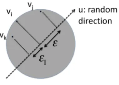
Fig. 3. Directionuis chosen randomly. The vectorvj−vkhas projection�1+�onuand it gets “assigned” tok. Letvi∈Z. For 1−δ/2 fraction of directionsu, there is a pointvj ∈Zi such that�vj−vi, u� ≥�1. Also
forδfraction of directionsu, there is a point in vk∈X such that�vk−vi, u� ≤ −�andvk is matched tovi
in the matchingMu. Thus for aδ/2 fraction of directions u, both events happen and thus the pair (vj, vk) satisfies �vj−vk, u� ≥ �1+�. Since vj ∈ Zi and vk ∈ X, we “assign” this vector vj−vk to point vk for
directionu, as a step towards building a cover centered atvk. Now we argue that for manyvk’s, the vectors assigned to it in this way form an (�1+�, δ|Z|/2|X|)-cover.
For each pointvi ∈Z, for δ/2 fraction of the directions uthe process above assigns a vector to a point in X for directionu according to the matching Mu. Thus on average for each direction u, at least δ|Z|/2 vectors get assigned by the process. Thus, for a random point inX, the expected measure of directions for which the point is assigned a vector is at leastδ|Z|/2|X|.
Furthermore, at most one vector is assigned to any point for a given directionu(since the assignment is governed by the matchingMu). Therefore at leastδ|Z|/4|X|fraction of the points inX must be assigned a vector forδ|Z|/4|X|=δτ /4 fraction of the directions.
We will define all such points ofX to be the setZ� and note that the size is at leastδ|Z|/4 as required.
✷
For the inductive proof of Lemma 7, it is useful to boost the covering probability of the cover obtained in Lemma 11 back up to 1−δ/2. This is achieved by invoking the boosting lemma as follows.
Corollary 12
If the vectors in the covers forZ� have length at most
�√d 4�log 8
τ δ+ 2
�
log2
δ then the(�1+�, τ δ/4)-covers forZ� are also(�1+�/2,1−δ/2)-covers.
Proof:
This follows from Lemma 10, since the loss in projection in this corollary is�/2 which should be less than γ�where�is the length of the vectors in the cover andγis defined as in Lemma 10. Solving for�yields the upper bound in the corollary.
✷
Though the upper bound on the length in the hypothesis appears complicated, we only use the lemma with�= Θ(1/√d) and constantδ. Thus, the upper bound on the length is Θ(1/�log(1/τ)).Furthermore, 1/τ will often be Θ(1).
4.3 Proof of Lemma 7
The proof of the lemma is carried out using Lemmas 10, and Corollary 12 in a simple induction. Before proving the lemma, let us restate a slight strengthening to make our induction go through.
Definition 9 Given a set of n points that is (σ, δ, c�)-matching covered by M with associated matching
graphM, we definev to be in the(k, ρ)-core,Sk,ρ, ifv is(k σ
2√d,1−ρ)-covered by points which are within k hops ofv in the matching graphM.
Claim 13
For constantδ, and everyk≥1, (1) |Sk,δ/2| ≥(δ4)
k
|X|
(2) or there is a pair(vi, vj)such that|vi−vj|= Ω(σ/√k)andviandvj are withinkhops in the matching graphM.
Proof:
Since the set of points is (σ, δ, c�)-matching covered, Lemma 4 implies that there exists a (σ, δ)-uniform
matching coverMof a subsetX of the point set. Fork= 1, the claim follows by settingS1,δ/2=X.
Now we proceed by induction onk.
Clearly if case 2 holds for k, then it also holds fork+ 1. So assume that case 1 holds for k, i.e., Sk,δ/2
satisfies the conditions of case 1. Composing the covers ofSk,δ/2with the matching coverMusing Lemma 11 Journal of the ACM, Vol. V, No. N, Month 20YY.
yields a cover for a set Z� of size at least δ4|Sk| with covering probability Θ(|Sk|/|X|), but with projection
length that is larger by�= Ω(1/√d). To finish the induction step the covering probability must be boosted to 1−δ/2 which by Lemma 10 decreases the projection length by
��log Θ(|X|/|Sk|)/√d=O(�√k/√d) (11) where � upper-bounds the length of the vectors in the cover. If this decrease is less than �/2, then the points inZ� are (k�/2 +�/2,1−δ/2)-covered andSk
+1,δ/2is large as required in case 1. Otherwise we have
�/2 = Θ(σ/√d) =O(�√k/√d), which simplifies to �≥gσ/√k, for some constantg and thus case 2 holds fork+ 1.
✷
Remark 7 An essential aspect of this proof is that thek-length path (fromMk) pieces together pairs from many different matchingsMu. Consider, for example, given a directionuand a matchingMuwith projection �onu, how we produce any pair of points with larger projection onu. Clearly, edges from the matchingMu do not help with this. Instead, given any pair (x, y)∈Mu, we extend it with a pair (y, z)∈Mu� for some
different directionu� where (y, z) also has a large projection onu.The existence of such a pair (y, z) follows
from the boosting lemma.
5. ACHIEVING
∆ = Ω(1
/
√
LOG
N
)
Theorem 1 requires ∆ = Ω(1/√logn) whereas we proved above thatset-findfinds large ∆-separated sets
for ∆ = Ω(log−2/3n). Now we would like to run set-find for ∆ = Ω(1/√logn). The main problem in
proving thatset-findsucceeds for larger ∆ is that our version of Lemma 7 is too weak. Before seeing how
to remedy this it is useful to review how the proof of Theorem 1 constrains the different parameters and results in a Θ(1/log2/3n) upper boundon ∆.
(1) In the proof of Lemma 7 we can continue to inductively assert case 1 (producing covered set Sk) of Claim 13 as long as the right hand side of Equation (11) is less thanσ/2√d,i.e., as long as �2
�1/k,
where�bounds the lengths of the vectors. (2) By the triangle inequality,�=O(√k∆).
(3) Deriving the final contradiction in the proof of Theorem 8 requires that exp(−k/∆)�1/n2.
The limit on the vector lengths in item 1, combined with item 2, requires thatk≤1/∆1/2, and thus item
3 constrains ∆ to beO(1/log2/3n).
The improvement derives from addressing the limit on vector lengths in item 1, which arises from the need to boost the covering probability forSk (whose size decreases exponentially ink) from Θ(|Sk|/|X|) to 1−δ/2 as detailed in Equation (11). Thus, we would like to prevent the size of Sk from decreasing below Ω(|X|). This will allow the induction to continue until the vectors have length Ω(1). To do so, we will use the fact that any point close to a point which is (�, δ)-covered is also (��, δ�)-covered where�� ≈�andδ� ≈δ.
This is quantified in Lemma 14.
Lemma 14 (Covering Close Points)
Supposev1, v2, . . .∈ �d form an(�, δ)-cover for v0. Then, they also form an (�−√tsd, δ−e−t
2/4
)-cover for everyv�
0such that|v0−v0�| ≤s.
Proof: Ifuis a random unit vector, Pru[�u, v0−v0�� ≥√tsd]≤e−t
2/4
. ✷
Remark 8 Lemma 14 shows that (�, δ) covers of a point are remarkably robust. In our context where we
can afford to lose Θ(1/√d) in projection length, even a Θ(1)-neighborhood of that point is well covered.
Definition 10 (ζ-proximate graph) A graphGon a set of pointsv1, . . . , vn∈ �dis calledζ-proximateif
for each edge(vi, vj)inG, satisfies|vi−vj| ≤ζ.A set of verticesS isnon-magnifying if|S∪Γ(S)|<|V|/2,
whereΓ(S) is the set of neighbors ofS inG.
Notice that for any setS if theζ-proximate graph is chosen to have edges between all pairs with distance at mostζ that ifT =V −S−Γ(S) thenS, T is aζ2-separated pair of sets. We will useζ2= ∆, thus if we ever find a non-magnifying setS of size Ω(n) then we are done.
We prove a stronger version of Lemma 7 where case 2 only occurs when vectors have Ω(1) length by ensuring in case 1 that the (k, δ/2)-core,Sk,δ/2, has size at least|X|/2.
The induction step in Lemma 11 now yields a set, which we denote byS�
k+1, of cardinalityδ|X|, which is
covered byX with constant covering probability and with projection length increased by Ω(1/√d). IfS�
k+1
is a non-magnifying set in theζ-proximate graph, we can halt (we have found aζ-separated pair of sets for theζ-proximate graph above). Otherwise, S�
k+1 can be augmented with Γ(Sk�+1) to obtain a setT of size
|X|/2 which by Lemma 14 is covered with projection length that is smaller byO(ζ/√d) and is contained in Sk+1,δ/2.
Then, we boost the covering probability at a cost of reducing the projection length byO(�/√d) where�is the length of the covering vectors. Thus whenζ �1, we either increase the projection length by Ω(1/√d) or �is too large or we produce a non-magnifying set. This argument yields the following enhanced version of Lemma 7:
Lemma 15
For every set of points X, that is(δ, σ)-uniform matching covered by Mwith associated matching graph M, and aζ-proximate graph on the points forζ≤ζ0(δ, c�, σ), at least one of the following is true for every
k≥1, whereg=g(δ, c�)is a positive constant.
(1) The(k, δ/2)-core,Sk,δ/2, has cardinality at least|X|/2
(2) There is a pair(vi, vj)with distance at mostk in the matching graphM, such that
|vi−vj| ≥g. (3) The set,S�
k�, is non-magnifying in theζ-proximate graph for somek� < k.
We can now prove Theorem 1. We use set-find with some parameter ∆ = Θ(1/√logn). If it fails to find a ∆-separated set the point set must have been (σ, δ, c�)-matching covered whereδ, c�, and σare Θ(1).
We first apply Lemma 4 to obtain a (σ, δ�)-uniform matching covered set X of size Ω(n). We then apply
Lemma 15 where the edges in theζ-proximate graph consist of all pairs inX whose�2
2distance is less than
someζ2= Θ(1/√logn). If case 3 ever occurs, we can produce a pair ofζ-separated of size Ω(n). Otherwise,
we can continue the induction until k= Ω(√logn) at which point we have a cover with projection length Θ(√logn/√d) consisting of vectors ofO(1) length. As in our earlier proof, this contradicts the assumption that set-find failed.
Thus, either set-find gives a ∆-separated pair of large sets, or for some k, the ζ-neighborhood of Sk, Γ(Sk), is small and thus,Sk, V −Γ(S�
k) forms a ζ-separated pair of large sets. Clearly, we can identify such anSk by a randomized algorithm that uses random sampling of directions to check whether a vertex is well covered.
This proves Theorem 1.
Remark 9 Lee’s direct proof that set-find [2005] produces Ω(1/√logn)-separated sets relies on the
fol-lowing clever idea: rather than terminating the induction with a non-magnifying set (in the ζ-proximate graph), he shows how to use the non-magnifying condition to bound the loss in covering probability. The main observation is that after cover composition, the covering probability is actually|Sk|/|Γ(Sk)|rather than our pessimistic bound of |Sk|/|X|. Thus by insisting on the invariant that |Γ(Sk)| = O(|Sk|), he ensures that the covering probability falls by only a constant factor, thus incurrring only a small boosting cost and allowing the induction to continue for k = Ω(1/∆) steps. Maintaining the invariant is easy since Sk can be replaced by Γ(Sk) with small cost in projection length using Lemma 14. The point being that over the course of the induction this region growing (replacingSk by Γ(Sk)) step only needs to be invoked O(logn) times.
6.
O
(
√
LOG
N
)
RATIO FOR SPARSEST CUTNow we describe a rounding technique for the SDP in (8) – (10) that gives an O(√logn)-approximation to sparsest cut. Note that our results on expander flows in Section 7 give an alternative O(√log
n)-approximation algorithm.
First we see in what sense the SDP in (8) –(10) is a relaxation for sparsest cut. For any cut (S, S)
consider a vector representation that places all nodes in S at one point of the sphere of squared radius (2|S|��S��)−1and all nodes in
|S|at the diametrically opposite point. It is easy to verify that this solution is feasible and has value��E(S, S)��/|S|��S��.
Since ��S��∈[n/2, n], we conclude that theoptimalvalue of the SDP multiplied by n/2 is a lower bound forsparsest cut.
The next theorem implies that the integrality gap isO(√logn).
Theorem 16
There is a polynomial-time algorithm that, given a feasible SDP solution with valueβ, produces a cut(S, S) satisfying��E(S, S)��=O(β|S|n√logn).
The proof divides into two cases, one of which is similar to that of Theorem 1. The other case is dealt with in the following Lemma.
Lemma 17
For every choice of constantsc, τwherec <1, τ <1/8there is a polynomial-time algorithm for the following task. Given any feasible SDP solution with β =�{i,j}∈E|vi−vj|2, and a node k such that the geometric ball of squared-radius τ /n2 around vk contains at least cn vectors, the algorithm finds a cut (S, S) with
expansion at mostO(βn/c).
Proof: Let d(i, j) denote|vi−vj|2, and when {i, j} is an edge ewe write we for d(i, j). The weights we turn the graph into a weighted graph.
LetX be the subset of nodes that correspond to the vectors in the geometric ball of radiusτ /n2 around
vk. The algorithm consists of doing a breadth-first search on the weighted graph starting fromX. Fors≥0 letVsbe the set of nodes whose distance fromX is at mosts, and letEsbe the set of edges leavingVs. We identifysfor which the cut (Vs, Vs) has the lowest expansion, say αobs, and output this cut.
The expansion of the cut (Vs, Vs) is
|Es| min�|Vs|,��Vs���. Since|Vs| ≥c·��Vs��, the expansion is at most
|Es|
c·��Vs��, allowing us to conclude|Es| ≥cαobs��Vs��for alls.
To finish, we need to show thatαobs=O(βn/c).
Since�i<jd(i, j) = 1, the triangle inequality implies that each node malso satisfies:
�
i,j
d(i, m) +d(j, m)≥1, which implies
�
j
d(j, m)≥1/2n. (12)
Separating terms corresponding toj∈X andj �∈X in (12) and usingcτ <1/8 we obtain for the special nodek:
�
j�∈X
d(j, k)≥ 1 2n−
τ n2 ·cn≥
3
8n. (13)
The Lemma’s hypothesis also says
�
e∈E
we=β. (14)
As we noticed in the proof of Corollary 2, each edgee={i, j} only contributes toEs for sin the open interval (s1, s2),wheres1=d(i, X) ands2=d(j, X). Triangle inequality implies that|s2−s1| ≤we.
Thus
β=�
e∈E we≥
�
s>0|
Es|ds≥
�
s>0
cαobs��Vs�� ds. Furthermore, we note that
�
s>0
�
�Vs�� ds=� i�∈X
d(i, X)≥� i�∈X
(d(i, k)− τ n2).
Thus, from equation (13) we have that
�
s>0
�
�Vs�� ds≥83n −n· τ n2 >
1 4n.
Combining the above inequalities, we obtainβ ≥cαobs/4n,or, in other wordsαobs=O(βn/c).
✷
Now, in case the conditions of Lemma 17 does not hold, we runset-find.
The following lemma ensures that for any point set that isc-spread and does not meet the conditions of Lemma 17 that the procedure proceeds to Step 2 ofset-findwith a reasonable probability for a value ofσ that is Ω(1).
Lemma 18
Given a c-spread set of points where no more than n/10 of them are contained in a ball of diameter1/10, there is aσ=O(c)such that Step 1 ofset-finddoes not HALT with probability at leastΩ(1).
Proof:
We begin with the following claim.
Claim 19
For at least1/20of the directions, at least1/20of the pairs are separated by at least1/90√din the projection.
Proof:
Consider a vertexvi. The number of pairs vi, vj where|vi−vj| ≥1/10 is at least 9(n−1)/10. Over all
pairs, the number is 9n(n−1)/10. For unordered pairs, this is 9n(n−1)/20.
For each such pair, the probability thatvi andvj fall at least 1/90√dapart is at least 1/3 from Lemma 5. Thus, the expected number of pairs that are separated by an interval of length 1/20√dis at least 9n(n−1)/60. Using the fact that the expected number can never be larger thann(n−1)/2, we see that with probability at least 9/120 at least 9n(n−1)/120 pairs are separated by at least 1/90√d. ✷
Notice that set-findwith σ = 1/180 only HALTS in step 1 if more than 90% of the nodes are within 1/180√d of the median point. This does not occur with probability more than 19/20. Thus, Set-Find
succeeds with Ω(1) probability.
✷
To finish, we observe that if the procedure fails in step 2, then the point set must be (σ,Θ(1),Θ(1)) matching covered. We can then use Lemma 15 to produce a cut or to derive a contradiction as we did before.
7. EXPANDER FLOWS: APPROXIMATE CERTIFICATES OF EXPANSION
Deciding whether a given graphGhas expansion at leastαis coNP-complete (Blum et al. [1981]) and thus has no short certificate unless the polynomial hierarchy collapses. On the other hand, the value of the SDP used in the previous sections gives an “approximate” certificate of expansion. Jerrum and Sinclair [1989] and then Leighton and Rao [1999] previously showed how to use multicommodity flows to give “approxi-mate” certificates; this technique was then clarified by Sinclair [1992] and Diaconis and Saloff-Coste [1993]. Their certificate was essentially an embedding of a complete graph into the underlying graph with minimal expansion. This certificate could certify expansion to within a Θ(logn) factor.
The results of this section represent a continuation of that work but with a better certificate: for any graph with α(G) =αwe can exhibit a certificate to the effect that the expansion is at least Ω(α/√logn). Furthermore, this certificate can be computed in polynomial time. The certificate involves using multicom-modity flows to embed (weighted) expander graphs. The previous approaches were the same except that the expander was limited to be the complete graph. In our approach, we can choose the expander which is the easiest to embed in the underlying graph.
We remark that this view led to recent faster algorithms of Arora, Kale and Hazad [2004] for approximating sparsest cuts. We note that this view essentially follows from SDP duality, in the sense that the certificate we use is a feasible solution to the dual of the semi-definite program that we used in previous sections.
In this discussion it will be more convenient to look at weighted graphs. For a weighted graphG= (V, W) in whichcij denotes the weight on edge{i, j} the sparsest cut is defined as
Φ(G) = min S⊆V:|S|≤n/2
�
i∈S,j∈Sci,j
|S|��S�� . We similarly defineα(G).
A word on convention. Weighted graphs in this section will be symmetric, i.e.,cij=cjifor all node pairs i, j. We call�jcij thedegreeof nodei. We say that a weighted graph isd-regular if all degrees are exactly d. We emphasize thatdcan be a fraction.
7.1 Multicommodity flows as graph embeddings
A multicommodity flow in an unweighted graph G= (V, E) is an assignment of a demand dij ≥0 to each node pairi, jsuch that we can routedij units of flow fromitoj, and can do this simultaneously for all pairs while satisfying capacity constraints. More formally, for eachi, j and each pathp∈ Pij there existsfp≥0 such that
∀i, j∈V �
p∈Pij
fp=dij (15)
∀e∈E �
p�e
fp≤1. (16)
Note that every multicommodity flow in G can be viewed as an embedding of a weighted graph G� =
(V, E�, dij) on the same vertex set such that the weight of edge{i, j}isdij. We assume the multicommodity
flow is symmetric, i.e.,dij =dji. The following inequality is immediate from definitions, since flows do not exceed edge capacities.
α(G)≥α(G�) (17)
The following is one way to look at the Leighton-Rao result whereKn is the complete graph onnnodes. The embedding mentioned in the theorem is, by (17), a certificate showing that expansion is Ω(α/logn).
Theorem 20 (Leighton-Rao [1999])
IfGis anyn-node graph withα(G) =α, then it is possible to embed a multicommodity flow in it with each fij =α/nlogn(in other words, a scaled version ofKn).