Attempt
Josine Verhagen & Eric-Jan Wagenmakers
University of AmsterdamAbstract
Replication attempts are essential to the empirical sciences. Successful repli-cation attempts increase researchers’ confidence in the presence of an effect, whereas failed replication attempts induce skepticism and doubt. How-ever, it is often unclear to what extent a replication attempt results in success or failure. To quantify replication outcomes we propose a novel Bayesian replication test that compares the adequacy of two competing hypotheses. The first hypothesis is that of the skeptic and holds that the effect is spurious; this is the null hypothesis that postulates a zero effect size, H0 : δ = 0. The second hypothesis is that of the propo-nent and holds that the effect is consistent with the one found in the original study, an effect that can be quantified by a posterior distribu-tion. Hence, the second hypothesis –the replication hypothesis– is given by Hr : δ ∼ “posterior distribution from original study”. The weighted
likelihood ratio between H0 and Hr quantifies the evidence that the data
provide for replication success and failure. In addition to the new test, we present several other Bayesian tests that address different but related ques-tions concerning a replication study. These tests pertain to the independent conclusions of the separate experiments, the difference in effect size between the original experiment and the replication attempt, and the overall con-clusion based on the pooled results. Together, this suite of Bayesian tests allows a relatively complete formalization of the way in which the result of a replication attempt alters our knowledge of the phenomenon at hand. The use of all Bayesian replication tests is illustrated with three examples from the literature. For experiments analyzed using thettest, computation of the new replication test only requires the t values and the numbers of participants from the original study and the replication study.
Introduction
In recent years, the field of psychology has come under increased scrutiny. The promi-nence of implausible results, research fraud, questionable research practices, lack of data sharing, confirmation bias, publication bias, and failure to replicate key findings have led some researchers to conclude that psychology is in a “crisis of confidence” (e.g., Pashler & Wagenmakers, 2012; see also Bones, 2012; Francis, in pressb; John, Loewenstein, & Prelec, 2012; Neuroskeptic, 2012; Simmons, Nelson, & Simonsohn, 2011; Wagenmakers, Wetzels, Borsboom, & van der Maas, 2011; Wicherts, Borsboom, Kats, & Molenaar, 2006). One of the proposed solutions to overcome this crisis is to re-emphasize the importance of indepen-dent replications (e.g., Asendorpf et al., 2013; LeBel & Peters, 2011; Nosek & Bar–Anan, 2012; Nosek, Spies, & Motyl, 2012; Yong, 2012). The increased emphasis on replications is evident from initiatives such aspsychfiledrawer.org, the new replication sections in Per-spectives on Psychological Science andAttention, Perception, & Psychophysics, the special issues on replications inSocial Psychology (Nosek & Lakens, 2013) andFrontiers in Cogni-tion(Zwaan & Zeelenberg, 2013), and the Open Science Framework project on reproducibil-ity.1 Spearheaded by Brian Nosek, the latter initiative combines the research efforts of over 80 researchers to try and replicate a selection of articles from the 2008 volumes of Journal of Experimental Psychology: Learning, Memory, & Cognition, Psychological Science, and theJournal of Personality and Social Psychology.
Now that the field is on the verge of a paradigmatic shift towards increased trans-parency and more replication attempts, new questions arise. Most acute is the question of how to judge and quantify replication success. Qualitatively, many aspects need to be con-sidered when it comes to deciding whether a replication attempt resulted in success or failure (Brandt et al., 2013). Did the researchers test a similar population of participants? Did the researchers alter the paradigm in a meaningful way? Here we ignore these qualitative judgments and focus instead on the main quantitative aspect: assuming the experimental design and data collection strategy are adequate, how does one analyze the data to measure the statistical evidence for success or failure of a replication attempt?
In classical or frequentist statistics, the success of a replication attempt is commonly decided upon by comparing the p values of the original experiment and the replication attempt. However, comparing p values is a practice that is fraught with problems, as a difference in significance does not always indicate that the difference is significant (Gelman & Stern, 2006; Nieuwenhuis, Forstmann, & Wagenmakers, 2011) and differences in power between the original and replicated study can lead to counter-intuitive conclusions. An alternative procedure is to compare the effect size estimates in the two studies directly, either by computing a p value or by inspecting confidence intervals (Cohen, 1988, 1990; Rosenthal & Rubin, 1990). One problem with this procedure is that it can be difficult to demonstrate a failure to replicate when the original experiment was so low in power that
1
Seehttp://www.openscienceframework.org/project/EZcUj/wiki/home.
This research was supported by an ERC grant from the European Research Council. Correspondence concerning this article may be addressed to Josine Verhagen, University of Amsterdam, Department of Psychology, Weesperplein 4, 1018 XA Amsterdam, the Netherlands. Email address: [email protected].
the confidence interval on effect size is relatively broad and almost covers zero (Asendorpf et al., 2013).
To overcome these and other limitations, Simonsohn (2013) recently proposed a two-step method. In the first two-step, one defines what constitutes a small effect (in terms of how detectable it is given the sample size in the original study). In the second step, one tests whether the effect in the replication attempt is smaller than this small effect; when the effect is smaller than small, one concludes that the replication attempt was not successful. One disadvantage of this method –and frequentist methods in general– is that it cannot quantify support in favor of the null hypothesis. Thus, if a replication attempt is indeed successful (or, in frequentist parlance, not unsuccessful) the Simonsohn procedure cannot easily quantify the strength of evidence that the data provide for this success.
A third way in which to analyze the results of a replication attempt is to conduct a meta-analysis and assume that the original study and the replication attempt are exchange-able (Rouder & Morey, 2011). To assess whether or not there is a true effect, a common measure of effect size is obtained by weighting the effect sizes in the respective studies by the precision with which they were measured. In general, meta-analyses are based either on a fixed-effect model or on a random-effects model. The fixed-effect model assumes that all factors that could influence the effect size are the same in all studies. Hence, variations in effect size are due solely to sampling error around the true effect size. In contrast, the random-effects model assumes that each study has its own factors influencing effect size, and therefore the effect sizes are similar but not identical across studies. Effect size differences between studies are therefore caused both by sampling error and by between-study variance, where the effect size for each individual study is assumed to be normally distributed around a mean (overall) effect size. The drawback of this latter approach is that between-study variance is difficult to estimate when the number of available studies is limited. This means that in case of a single replication attempt, the random-effects approach is not feasible.
In Bayesian statistics, the success of a replication attempt has been decided upon using procedures that mimic those in the frequentist toolkit. For instance, based on the replication attempt one can quantify evidence for and against the null hypothesis using a default Bayesian hypothesis test (Dienes, 2011; Jeffreys, 1961; Kass & Raftery, 1995; Lee & Wagenmakers, 2013). This test answers the question “Is the effect present or absent in the data from the replication attempt?”. When the test outcome supports the null hypothesis, this can be taken as evidence for replication failure (e.g., Shanks et al., 2013; Ullrich, Krueger, Brod, & Groschupf, in press; Wagenmakers, Wetzels, Borsboom, van der Maas, & Kievit, 2012). Despite its intuitive appeal, this default Bayes factor hypothesis test often does not relate the data of the replication attempt to the data from the original experiment (but see Dienes, 2011). Consequently, the comparison of Bayes factors and p values share the same limitation: when the original experiment yields support in favor of the alternative hypothesis, and the replication attempt yields support in favor of the null hypothesis, this does not necessarily signal support for the assertion that the replication attempt differs from the original experiment.
To overcome this limitation, Bayarri and Mayoral (2002b) developed a Bayesian hy-pothesis test to assess whether the difference in effect size between the original experiment and the replication attempt is equal to zero (i.e.,H0) or not (i.e.,H1). This test answers the question “Are the effects from both studies of the same size?”. When the test outcome
sup-ports the null hypothesis, this can be taken as evidence for exact replication. The limitation of this procedure –which it shares with frequentist comparisons of effect size– is that it can be difficult to find evidence for either hypothesis in case of a low-powered experiment. The example used in Bayarri and Mayoral (2002b) makes this clear: with 10 participants per condition, even an exact replication does not yield a test result that supports the replication hypothesis in a compelling fashion.
Finally, the fixed-effect Bayesian meta-analysis test (Rouder & Morey, 2011) assesses the extent to which the combined data from all pertinent studies provides evidence for or against the null hypothesis of no effect. This test answers the question “When we pool the information from all experiments, do the data support the absence or the presence of the effect?”. This Bayesian test assumes that all experiments are exchangeable. Specifically, it assumes that each experiment was correctly executed in a purely confirmatory setting (De Groot, 1956/in press; Wagenmakers et al., 2012); it assumes that the experiments are uncontaminated by publication bias, hindsight bias, and confirmation bias; it also assumes that each experiment has the exact same underlying effect size. Each of these assumptions may be questioned, particularly by skeptics who have grounds to doubt the reproducibility of the findings from the original experiment.
Here we propose a new Bayesian test for replication success. Inspired by the work of Simonsohn (2013) and Dienes (2011), we seek to quantify the success or failure of a replication attempt. Given that the original experiment reported a significant effect, this test addresses the question “Is the effect from the replication attempt comparable to what was found before, or is it absent?”. Our test is based on a straightforward adaptation of the standard Bayesian hypothesis test, using the data from the replication attempt to pit against one another the following two hypotheses: first, the null hypothesis H0 – this represents the idealized belief of a skeptic, who has reason to doubt the presence of a particular effect. For the null hypothesis, effect size equals zero, that is, H0:δ = 0.2 The second hypothesis is the replication hypothesis Hr – this represents the idealized belief of a proponent, often
the person who carried out the original experiment but more generally any researcher who feels that the results of the original experiment(s) can be trusted.3
Here is where our test deviates from the default Bayesian hypothesis tests advocated in psychology by Rouder, Morey, and ourselves (Rouder, Speckman, Sun, Morey, & Iver-son, 2009; Rouder, Morey, Speckman, & Province, 2012; Wagenmakers, van der Maas, & Grasman, 2007; Wetzels & Wagenmakers, 2012; Wetzels, Grasman, & Wagenmakers, 2012). In the default Bayesian hypothesis tests, H0 is compared against the alternative hypothesis H1 that features a relatively vague belief about effect size, often quantified by a Gaussian distribution centered on zero. This default assignment of belief is blind to the earlier experiments that have been observed (Dienes, 2011). In contrast, the ideal-ized belief of the proponent is tightly linked to the outcome of the original experiment. As outlined below, we assume that the idealized belief of the proponent is given by the posterior distribution on effect size as obtained from the original experiment. Hence, our replication test assesses the extent to which the data from the replication attempt are more
2
It is possible to relax this assumption and also allow small values ofδsurrounding zero (Morey & Rouder, 2011), but we will not pursue such an analysis here.
3
The general idea of specifying the alternative hypothesis based on results from earlier studies was also put forward and implemented by Dienes (2011) and Bem, Utts, and Johnson (2011).
likely under the skeptic’s hypothesis H0 : δ = 0 or the proponent’s replication hypothesis Hr :δ ∼“posterior distribution from original study”. The default test and our replication
test address important yet complementary questions regarding the interpretation of data from replication attempts. To reiterate, the default test addresses the question “Given that we know relatively little about the expected effect size beforehand, is the effect present or absent in the replication attempt?”, and our test addresses the question “Is the effect simi-lar to what was found before, or is it absent?”. The two tests therefore represent extremes on a continuum of sensitivity to past research; the default test completely ignores the out-comes of an earlier experiment, whereas the replication test takes these outout-comes fully into account. The new test also deviates from the test for equality of effect sizes (Bayarri & Mayoral, 2002b) because the latter test does not take into account the skeptic’s hypothesis that the effect is absent. Finally, the new test deviates from the fixed-effect meta-analysis test (Rouder & Morey, 2011), because, from a skeptic’s position, the replication attempt is not exchangeable with the original experiment.
For concreteness and simplicity, the remainder of this article focuses on experiments analyzed using the t test. We first describe the existing Bayesian tests as they apply to replication attempts. Subsequently, we discuss the new Bayesian replication test in more detail and then explain how the posterior distribution can be derived from thettest results of the original experiment. Next we present a simulation study to demonstrate that the test works as intended and compare its results to those obtained from existing Bayesian tests. Finally, we apply each Bayesian test to three example findings from the published literature: the finding that women prefer men in red (Elliot et al., 2010), the finding that priming participants with concepts related to intelligence makes them act more intelligently (Dijksterhuis & van Knippenberg, 1998; LeBoeuf & Estes, 2004; Shanks et al., 2013), and the finding that negative priming is observed even when the prime was unattended (Milliken, Joordens, Merikle, & Seiffert, 1998; Neill & Kahan, 1999).
Bayes Factor Hypothesis Tests
Consider a standard one-samplettest for the difference between two dependent mea-suresY1 andY2. Assume that both scores are normally distributed and that the means and variances are unknown. In this case, the quantity t = (¯y1 −y¯2)/(s/
√
N) has a Student-t distribution with df = N −1 degrees of freedom, where ¯yi is the mean score on measure
Yi,sis the standard deviation of the difference betweenY1 andY2, andN is the number of observations. The effect size δ equals (¯y1−y¯2)/s=t/
√ N.4
Under the null hypothesis H0:δ = 0, the distribution oftis symmetric and centered at zero. Under the hypothesis of a specific alternative effect sizeH1:δ=δ1, the distribution of tis non-central with non-centrality parameter ∆1=δ1
√
N. The modelsH0 and H1 are each defined by a single specific effect size. Hence is it straightforward to compute, for each model, the probability of the observed data under the hypothesized effect size. The ratio of these probabilities is a likelihood ratio (Royall, 1997), and it quantifies the extent to which
4
For a two sample t test, for equal variances replace s with sp =
p
((n1−1)s21+ (n2−1)s22)/(n1+n2−2), N withNp = 1/(1/n1+ 1/n2) and df withdfp=n1+n2−2,
whereniis the number of participants in groupi. For unequal variances replaces
√
Nwithps2
1/n1+s22/n2
the observed data Y are more likely to have occurred under H1 relative to H0:
LR10=
p(Y | H1) p(Y | H0)
= tdf, δ1 √
N(tobs)
tdf(tobs)
, (1)
where tdf, δ 1
√
N(tobs) is the ordinate of the non-central t-distribution and tdf(tobs) is the
ordinate of the centralt-distribution, both withdf degrees of freedom and evaluated at the observed value tobs.
The problem with this analysis is that the exact alternative effect size δ1 is never known beforehand. In Bayesian statistics, this uncertainty aboutδis addressed by assigning it a prior distribution. Prior distributions reflect the relative plausibility of the entire range of different effect sizes. For instance, in the absence of subject-specific knowledge about the phenomenon of interest, a default prior distribution is H1 : δ ∼ N(0,1), a standard normal distribution (Rouder et al., 2009): this distribution reflects the belief that effect size is likely to be close to zero, and any positive value is just as likely as its corresponding negative value. Other prior distributions are possible and they will yield different results.
After assigning δ a prior distribution, the immediate computation of the likelihood ratio (Equation 1) is frustrated by the fact that H1 is now a composite hypothesis, re-flecting an entire distribution of effect sizes instead of a single value. Mathematically, this complication is overcome by computing a weighted average of likelihood ratios across all possible values of effect size, where p(δ | H1) serves as the weight function. To compute this weighted average, an integral is taken with respect to effect size. The resultant average likelihood ratio is better known as the Bayes factor:
B10=
p(Y | H1) p(Y | H0)
=
R
p(Y |δ,H1)p(δ| H1) dδ p(Y | H0)
=
Z t
df, δ√N(tobs)p(δ| H1) dδ
tdf(tobs)
=
Z
LR10p(δ| H1) dδ.
(2)
Interpretation of the Bayes factor
The Bayes factor B10 quantifies the strength of the evidence that the data provide for H1 versus H0. When B10 = 11.5, for instance, the data are 11.5 times more likely to have occurred under H1 than under H0. Values of B10 lower than 1 support H0. In such cases, a better appreciation for the strength of evidence in favor of H0 can be obtained by computing B01 = 1/B10 (Rouder & Morey, 2012); for instance, when B10 = .04 this means that the data from the replication attempt are 1/.04 = 25 times more likely to have occurred underH0 than underH1.
The outcome of a Bayes factor test is not a decision. Instead, “its function is to grade the decisiveness of the evidence.” (Jeffreys, 1961, p. 432). Although the decisiveness of evidence has a continuous scale, Jeffreys (1961) proposed a series of discrete categories that
facilitate scientific communication (see also Wetzels et al., 2011). In particular, Jeffreys (1961) argued that values of B10 in between 3 and 1/3 are anecdotal or “not worth more than a bare mention”. This label is helpful because it explicitly allows for the possibility that the data are ambiguous, and because it protects researchers from over-interpreting their findings. Note that, in contrast to p values, Bayes factors are able to quantify evidence in favor of a null hypothesisH0. This is particularly relevant for replication research.
Three Extant Bayes Factors for the Analysis of Replication Attempts
This section details three extant Bayes factor tests that can be used to analyze the results of a replication attempt. This will set the stage for the introduction of our new test. As discussed above, these Bayes factors address different but related questions. Specifically, the default Bayes factor test addresses the question “Is the effect present or absent in the replication attempt?”, the Bayes factor test for equality of effect sizes addresses the question “Are the effect sizes from the original experiment and the replication attempt the same?”, and the fixed-effect meta-analysis test addresses the question “When we treat all pertinent studies as exchangeable, is the effect present overall?”.
1. Independent JZS Bayes Factor Test: “Is the Effect Present or Absent in the Replication Attempt?”
The default Bayes factor test assesses the evidence for the presence or absence of an effect in isolation, without recourse to the original experiment. The test compares the null hypothesis that effect size δ is zero against an alternative hypothesis that effect size is not zero. The alternative hypothesis, however, needs to be specified explicitly and precisely. Because the alternative hypothesis is so well-specified, the Bayes factor can quantify the extent to which the data support that hypothesis versus the null hypothesis. Consequently, Bayes factors have two concrete advantages over classical null hypothesis significance testing by means of p-values. The first advantage is that Bayes factors can quantify evidence in favor of the null hypothesis (Rouder et al., 2009), something that is of primary importance in hypothesis tests for replication attempts; the second advantage is that Bayes factors are relatively reluctant to reject the null hypothesis when it provides a poor fit – after all, the alternative hypothesis may provide a fit that is just as poor or even worse (Edwards, Lindman, & Savage, 1963; Sellke, Bayarri, & Berger, 2001).
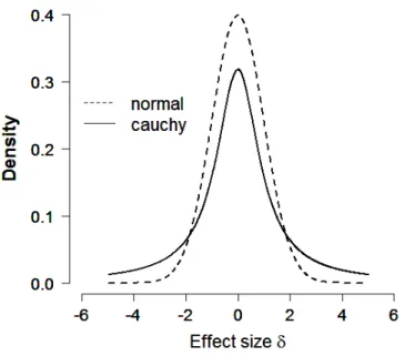
To specify the alternative hypothesis that the effect size is different from zero (i.e., H1 : δ 6= 0), the default test assigns a general-purpose prior to effect size. Most default general-purpose priors are centered on zero and have fat tails (for details see Bayarri, Berger, Forte, & Garc´ıa-Donato, 2012). For thettest, a popular prior is the standard Cauchy prior δ∼Cauchy(0,1) (Rouder et al., 2009). As can be seen in Figure 1, the Cauchy distribution has fatter tails than the standard Normal distribution, and assigns highest probability to effect sizes between−2 and 2, which contains most effect sizes in psychology. Together with uninformative priors on the means and variances, this popular prior set-up is also known as the Jeffreys-Zellner-Siow (JZS) prior (Liang, Paulo, Molina, Clyde, & Berger, 2008; Zellner, 1986; Zellner & Siow, 1980; Bayarri & Garc´ıa-Donato, 2007; Bayarri et al., 2012).
After explicitly specifying the alternative hypothesis, the JZS Bayes factor is now computed as the ratio of two probabilities: the probability of the observed data given the null
Figure 1. The Cauchy distribution and the standard Normal distribution.
hypothesisH0 :δ= 0, and the probability of the observed data givenH1 :δ ∼Cauchy(0,1). As explained in the previous section, the latter probability is obtained by averaging the likelihood of the observed data with respect to the Cauchy prior distribution. The resulting Bayes factor,B10, quantifies the extent to which the observed data supportH1 overH0:
B10=
p(Y | H1) p(Y | H0)
=
R
p(tobs |δ)p(δ| H1) dδ p(tobs |δ= 0)
=
R
tdf,δ√
N(tobs)p(δ | H1) dδ
tdf(tobs)
=
R
tdf,δ√
N(tobs)Cauchy (0,1) dδ
tdf(tobs)
.
(3)
As indicated in the previous section, values of B10 higher than 1 indicate support for H1, whereas values lower than 1 indicate support forH0(i.e., something that is not possible withp-values).
2. Equality-of-Effect-Size Bayes Factor Test: “Does the Effect Size in the Replication At-tempt Equal the Effect Size in the Original Study?”
Both proponents and skeptics should be interested in the assessment of whether the effect size from an original experiment equals that of the replication attempt. Bayarri and
Mayoral (2002b) proposed a Bayes factor test to quantify the evidence for the hypothesis that the effect sizes from two experiments are equal versus the hypothesis that they are not. In their test, Bayarri and Mayoral (2002b) assumed that there was one true underlying effect sizeµ, from which the effect sizes in the original (δorig) and replicated study (δrep) deviate
with varianceτ2. The test for the effect size difference between the original experiment and the replication attempt therefore amounts to testing whether this variance τ2 is equal to zero:
B01=
p(Yorig, Yrep | H0) p(Yorig, Yrep | H1)
= p(Yorig, Yrep|δorig, δrep)p(δorig, δrep|τ 2 = 0)
R
p(Yorig, Yrep|δorig, δrep)p(δorig, δrep|τ2)p(τ2| H1) dτ2 .
(4)
The statistical details of this equality-of-effect-size Bayes factor are reported in Ap-pendix B. Note that for this particular Bayes factor, the null hypothesis corresponds to a lack of difference between the effect sizes. Hence, evidence in favor of the null hypothesis is indicative of a successful replication. For consistency of interpretation with the other Bayes factors, for which the null hypothesis represents replication failure instead of success, the remainder of this paper reports this Bayes factor asB01 instead of asB10.
3. Fixed-Effect Meta-Analysis Bayes Factor Test: “When Pooling All Data, is the Effect Present or Absent?”
When it is plausible to treat a series of experiments as exchangeable, and when there is no scepticism about the original experiment, one may wonder about the extent to which the pooled data support the hypothesis that a particular effect is present or absent. This question can be addressed by a fixed-effect meta-analytic Bayes factor (Rouder & Morey, 2011). The test assumes that there is a single true underlying effect size, and that the observed effect sizes in the various experiments fluctuate around this true value due only to sampling variability. The JZS Bayes factor described earlier can be generalized to includeM independent experiments. As before, a Cauchy distribution is taken as a prior distribution forδ in each experiment.
As the experiments are independent, this results in a product of the terms in Equa-tion 3 over allM studies:
B10=
p(Y1, . . . , YM | H1) p(Y1, . . . , YM | H0)
=
R
p(t1, . . . , tM |δ)p(δ | H1) dδ p(t1, . . . , tM |δ= 0)
=
R hQM
m=1p(tm |δ)
i
p(δ | H1) dδ
QM
m=1p(tm |δ= 0)
=
R hQM
m=1tdfm,δm
√
N(tm) i
Cauchy (0,1) dδ
QM
m=1tdf(tm)
.
The resulting meta-analytic Bayes factor quantifies the evidence that the data provide for the hypothesis that the true effect size is present (i.e., H1) versus absent (i.e., H0). Hence, a high Bayes factor B10 indicates that the evidence from the pooled data support the hypothesis that a true effect is present.
The New Bayes Factor Test for Replication Success
In this section we outline the rationale of our novel Bayesian replication test as it applies to the common Student t test. The central idea is that we can pit against each other two hypotheses for dataYrep from a replication attempt: the skeptic’s null hypothesis
H0 and the proponent’s replication hypothesisHr. The relative support of dataYrep forH0 versus Hr is quantified by a Bayes factor, whose computation requires that we specify Hr
precisely. As explained earlier, the new replication test definesHr to be the idealized belief of a proponent, that is, the posterior distribution from the original experiment,p(δ |Yorig).
Given this definition ofHr, a straightforward way to approximate the desired Bayes
factor Br0 is to draw M samples from p(δ | Yorig), compute a likelihood ratio for each
sample, and then average the likelihood ratios: Br0 =
p(Yrep | Hr)
p(Yrep | H0)
=
R
p(Yrep|δ,Hr)p(δ |Yorig) dδ
p(Yrep | H0)
=
R
tdf,δ√
N(trep)p(δ |Yorig) dδ
tdf(trep)
≈ 1 M
M X
i=1
tdf,δ(i)√N(trep)
tdf(trep)
, δ(i)∼p(δ|Yorig),
(6)
where trep denotes the observed tvalue in the replication attempt, and the approximation
in the last step can be made arbitrarily close by increasing the number of samples M. As detailed in a later section, only the tvalue torig and the degrees of freedom from
the original experiment are used to determine p(δ | Yorig); together with the summary
data from the replication attempt (i.e., trep and df) this provides all information required
to obtain Br0 as indicated in the final step from Equation 6. R code to calculate Br0 is available on the first author’s website.5
A Frequentist Replication Factor
Our new test is Bayesian but it is possible to develop frequentist analogues. One idea is to compute a likelihood ratio, as in Equation 1, and plug in the single best estimate of effect size as an instantiation of the replication hypothesis: δ = ˆδ | Yorig. A major
drawback of this procedure is that it is based on a point estimate, thereby ignoring the precision with which the effect size is estimated – and precisely estimated effect sizes lead to more informative tests. A more sophisticated idea is to bootstrap the original data set (Efron & Tibshirani, 1993) and obtain, for each bootstrapped data setYorig?,i , a corresponding
5
best estimate of effect size, ˆδ?,i |Yorig?,i . The distribution of these bootstrapped effect size estimates can be viewed as a poor man’s Bayesian posterior distribution. Next, a frequentist counterpart of Equation 6 can be obtained by computing a likelihood ratioLR?,i0r for every one of K bootstrapped effect size estimates ˆδ? |Yorig? , and then averaging these likelihood ratios to obtain a “frequentist replication factor”: F RF0r ≈ K1 PKi=1LR
?,i
0r. From Prior to Posterior to Prior to Posterior: Bayesian Updating
So far our analysis assumed that we have available the posterior distribution of the effect size obtained from the original study, p(δ | Yorig). This posterior is a compromise
between the prior distribution and the information in the data, and we deal with these two ingredients in turn. First, for the prior, we assume that before seeing the data from the original study the proponent started out with an uninformative, flat prior distribution on effect size. This is an assumption of convenience that is, fortunately, not at all critical: under general conditions, the data overwhelm the prior and dissimilar prior distributions result in highly similar posterior distributions (Edwards et al., 1963). The flat distribution is convenient to use because it allows a connection to the frequentist literature on confidence intervals.
Second, for the information in the data from the original experiment, we only need the tvalue and the degrees of freedom. Under the assumption of a flat prior, we can then obtain the posterior distribution for effect size. This posterior distribution is a mixture of non-centraltdf,∆(tobs)-distributions with non-centrality parameters ∆ =δ
√
N. To approximate this posterior distribution, we first use an iterative algorithmic search procedure (Cumming & Finch, 2001) to obtain a 95% frequentist confidence interval for effect size; next we interpret this 95% confidence interval as a 95% Bayesian credible interval (Lindley, 1965; Rouanet, 1996) and assume the posterior is normally distributed. As demonstrated in Appendix A, the normal approximation to the posterior is highly accurate, even for small sample sizes.
For the proponent then, the Bayesian updating sequence proceeds as follows: before observing the data from the original experiment, the proponent has an uninformative prior distribution on effect size,p(δ); when the data from the original experiment become avail-able, this prior distribution is updated to a posterior distribution,p(δ|Yorig); this posterior
reflects the proponent’s idealized belief about δ after observing the original experiment, and it is used as a prior for our Bayesian replication test, as per Equation 6. Finally, the posterior-turned-prior p(δ |Yorig) is confronted with the data from the replication attempt
and is updated to another posterior, p(δ |Yrep, Yorig).6
Simulation Study
To illustrate the behavior of the different Bayesian tests, Tables 1-4 show the results of a simulation study based on a one-sample ttest. The study systematically varied the t values and sample sizes for an original experiment and a replication attempt, resulting in
6
From the point of view of the skeptic, the updating process ignores the possibility that the effect is absent; in addition, there may be reasons to doubt that Yorig is tainted by publication bias or hindsight
bias. Our replication test quantifies the extent to which the replication dataYrep support the proponent’s
different replication test results. The rows are defined by the tvalues in the original study and feature original sample sizes of 50 (upper half) and 100 (lower half). The columns are defined by thetvalues in the replication attempt and feature replication sample sizes of 50 (left half) and 100 (right half).
New Bayes Factor Replication Test
For the Bayes factor replication test, the simulation study highlights three intuitive regularities. First, evidence for successful replication increases when the replicated effect size is further away from the skeptic’s belief that the effect size is zero. In Table 1, each separate row shows that Br0 increases withδrep. Second, evidence for successful replication
increases when the replicated effect size δrep is closer to the observed effect size δorig. For
example, within the (norig = nrep = 50) quadrant, consider the column with a replicated
effect size of .28. Within this column, the Bayes factor is highest (i.e., 4.94) when the original effect size is also .28 (i.e., the second row). The next column, with a replicated effect size of .42, shows a similar effect: again, the Bayes factor is highest (i.e., 46) when the original effect size is also .42 (i.e., the third row). This regularity is apparent in all quadrants of Table 1.
Third, more decisive test outcomes are obtained when the sample size in the repli-cation attempt is large. With increased sample size, there is more support for the null hypothesis in case the replication effect size is close to zero, and there is more support for the replication hypothesis in case the replication effect size equals or exceeds the orig-inal effect size. For example, the lower left panel in Table 1 shows that Br0 = 5.67 with norig =nrep = 50, δorig =.3, and δorig =.28; the lower right panel shows that for
compa-rable effect sizes but twice as many participants, a more informative outcome is obtained: Br0 = 53.69. A similar but much weaker regularity is apparent when the sample size of the original experiment is increased. These Bayes factor results are similar to those ob-tained from the method proposed by Dienes (2011), who used a normal prior distribution with meanMorig and standard deviationMorig/2, whereMorigis the mean observed in the
original experiment.
Although the results of the Bayes factor replication test are on a continuous scale we can compare them to the common practice of labeling replications as success or failure based on thepvalue from the replicated study. According to a conventional two-sidedttest with 50 or 100 participants and an alpha level of.05, the null hypothesis should be rejected at a t value near 2. In Table 1, the results for the columns where trep = 2 demonstrate
that this corresponds to the data being at worst 0.53 and at best 5.67 times more likely to occur under the replication hypothesis than under the null hypothesis. Across most entries in Table 1, a replicationt value of 2 yields evidence that favors the replication hypothesis, albeit in rather modest fashion (Jeffreys, 1961). This illustrates the well-known fact that the p value overestimates the evidence against the null hypothesis (Edwards et al., 1963; Sellke et al., 2001). The overestimation occurs because the p value does not take into account the adequacy of the alternative hypothesis; when both the null hypothesis and the alternative hypothesis provide an equally poor account of the data, the p value indicates that the null hypothesis should be rejected. For the same data, the Bayesian replication test will correctly indicate that the data are ambiguous.
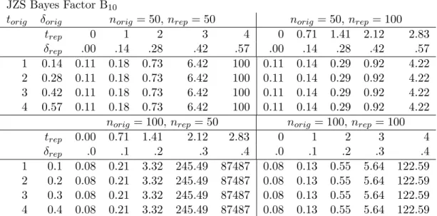
Replication Bayes Factor Br0
torig δorig norig= 50, nrep = 50 norig= 50, nrep = 100
trep 0 1 2 3 4 0.00 0.71 1.41 2.12 2.83
δrep .00 .14 .28 .42 .57 .00 .14 .28 .42 .57
1 0.14 0.55 1.17 3.87 17.71 96 0.41 1.53 18.82 585 44343 2 0.28 0.26 0.91 4.94 36.50 311 0.15 1.09 25.64 1513 222076 3 0.42 0.08 0.44 3.88 46.01 620 0.03 0.42 18.28 2019 576871 4 0.57 0.02 0.14 1.94 36.49 770 0.00 0.09 7.28 1449 783072
norig= 100, nrep = 50 norig= 100, nrep = 100
trep 0.00 0.71 1.41 2.12 2.83 0 1 2 3 4
δrep .00 .1 .2 .3 .4 .00 .1 .2 .3 .4
1 0.1 0.69 1.05 1.86 3.75 8.24 0.55 1.17 3.97 20.28 141
2 0.2 0.42 0.89 2.20 6.11 18.29 0.26 0.91 5.08 42.25 472 3 0.3 0.19 0.54 1.87 7.19 29.45 0.08 0.44 3.97 53.68 966 4 0.4 0.06 0.24 1.15 6.13 34.51 0.01 0.13 1.93 42.24 1220
Table 1: Results from the Bayes factor replication test Br0 applied to different values oftorig,trep,
norig, andnrep. The rows are defined by thetvalues in the original study and corresponding effect sizes for original sample sizes of 50 (upper half) and 100 (lower half). The columns are defined by thetvalues in the replication attempt and corresponding effect sizes for replication sample sizes of 50 (left half) and 100 (right half).
Independent JZS Bayes Factor Test
Table 2 shows the outcomes for the JZS Bayes factor test. For the evaluation of the results from the replication attempt, the JZS Bayes factor test ignores the findings that were obtained in the original study. Hence, within each of the four quadrants all rows in Table 2 are identical. The JZS Bayes factors show increasing evidence for the null over the alternative hypothesis when the effect size in the replicated study increases. This increase is stronger for larger sample sizes.
The results show that if the effect size of the replication attempt is in the same direction as that of the original experiment, the default test generally yields weaker evidence againstH0 than does the replication test. For example, whenδrep =.28 andnorig =nrep=
50, the default test yields an inconclusive Bayes factor of.73. The replication test, however, yields more informative Bayes factors ranging from 1.94 to 4.94 in favor of the alternative hypothesis. This discrepancy between the default JZS Bayes factor test and the Bayes factor replication test is due to the fact that the definition of the alternative hypothesis is more informative in the replication test, featuring a prior that is not centered on zero. Equality-of-Effect-Size Bayes Factor Test
Table 3 shows the outcomes for the Bayes factor test for the equality of effect sizes. As expected, the Bayes factor for equality of effect sizes is highest when the effect sizes are equal and sample size is large. As mentioned earlier, compelling evidence for equality of effect sizes can be obtained only for sample sizes that are relatively large. Furthermore, note that the Bayes factor for equality of effect sizes is relatively insensitive to their deviation
JZS Bayes Factor B10
torig δorig norig = 50,nrep = 50 norig = 50,nrep = 100
trep 0 1 2 3 4 0 0.71 1.41 2.12 2.83
δrep .00 .14 .28 .42 .57 .00 .14 .28 .42 .57
1 0.14 0.11 0.18 0.73 6.42 100 0.11 0.14 0.29 0.92 4.22
2 0.28 0.11 0.18 0.73 6.42 100 0.11 0.14 0.29 0.92 4.22
3 0.42 0.11 0.18 0.73 6.42 100 0.11 0.14 0.29 0.92 4.22
4 0.57 0.11 0.18 0.73 6.42 100 0.11 0.14 0.29 0.92 4.22
norig = 100,nrep = 50 norig= 100, nrep = 100
trep 0.00 0.71 1.41 2.12 2.83 0 1 2 3 4
δrep .0 .1 .2 .3 .4 .0 .1 .2 .3 .4
1 0.1 0.08 0.21 3.32 245.49 87487 0.08 0.13 0.55 5.64 122.59 2 0.2 0.08 0.21 3.32 245.49 87487 0.08 0.13 0.55 5.64 122.59 3 0.3 0.08 0.21 3.32 245.49 87487 0.08 0.13 0.55 5.64 122.59 4 0.4 0.08 0.21 3.32 245.49 87487 0.08 0.13 0.55 5.64 122.59
Table 2: Results from the independent JZS Bayes factor test B10applied to replication attempts for
different values oftorig, trep, norig, and nrep. The rows are defined by thet values in the original study and corresponding effect sizes for original sample sizes of 50 (upper half) and 100 (lower half). The columns are defined by thetvalues in the replication attempt and corresponding effect sizes for replication sample sizes of 50 (left half) and 100 (right half). Because the test ignores the results from the original study, within each quadrant all rows are identical.
from zero. For example, within the (norig=nrep = 50) quadrant, consider the entries where
δorig =δrep = (.14, .28, .42, .57). The associated Bayes factors from test for equality of effect
sizes areB01= (8.22,8.05,8.00,7.21) – the extent to which the effect sizes deviate from zero does not influence the test, because the test ignores the skeptic’s hypothesis that effect size is zero. In contrast, for those same table entries, the Bayes factor replication test –pitting the proponent’sHragainst the skeptic’sH0– yields evidence that greatly increases with the deviation of δ from 0: Br0 = (1.17,4.94,46,770). This qualitative difference between the two tests reflects the fact that they address different substantive questions.
Fixed-Effect Meta-Analysis Bayes Factor Test
Table 4 shows the outcomes for the fixed-effect meta-analysis Bayes factor. This test pools the data from the original experiment and the replication attempt and determines whether the effect is present or absent overall. As expected, the meta-analytic Bayes factor is relatively high when both effect sizes are large. Whenever one of the effect sizes is low, the other one has to be high to compensate and produce a Bayes factor in favor of the effect. Studies with large sample size have more of an influence on the final outcome than do studies with small sample sizes.
In contrast to the new replication test, the meta-analytic Bayes factor treats the data from the original study and the replication attempt as exchangeable. This yields different conclusions, particularly in cases where a high effect size in the original study provides sufficient evidence to compensate for a small effect size in the replication attempt. These situations hold in the lower left corners for each of the quadrants of Table 4. For example,
Equality-of-Effect-Size Bayes FactorB01
torig δorig norig = 50,nrep = 50 norig= 50, nrep = 100
trep 0 1 2 3 4 0.00 0.71 1.41 2.12 2.83
δrep .00 .14 .28 .42 .57 .00 .14 .28 .42 .57
1 0.14 6.42 8.22 6.29 2.96 1.01 6.75 9.37 6.79 2.63 0.48
2 0.28 3.12 6.44 8.05 6.27 3.14 2.58 6.68 9.26 6.79 2.42
3 0.42 0.97 3.18 6.44 8.00 6.03 0.54 2.62 6.66 9.26 6.44
4 0.57 0.20 1.01 3.25 6.45 7.21 0.07 0.58 2.66 6.69 8.87
norig = 100,nrep = 50 norig= 100, nrep= 100
trep 0.00 0.71 1.41 2.12 2.83 0 1 2 3 4
δrep .0 .1 .2 .3 .4 .0 .1 .2 .3 .4
1 0.1 7.97 9.34 7.93 4.81 2.12 8.89 11.44 8.86 4.22 1.23
2 0.2 4.92 8.06 9.38 7.84 4.84 4.34 9.07 11.36 8.79 4.22
3 0.3 2.21 4.99 7.92 9.24 7.86 1.27 4.32 8.98 11.40 8.72
4 0.4 0.72 2.22 5.02 7.94 8.79 0.24 1.33 4.38 9.00 11.06
Table 3: Results from the Bayes factor for equality of effect sizes B01 applied to different values
of torig, trep, norig, and nrep. The rows are defined by the t values in the original study and corresponding effect sizes for original sample sizes of 50 (upper half) and 100 (lower half). The columns are defined by the t values in the replication attempt and corresponding effect sizes for replication sample sizes of 50 (left half) and 100 (right half).
within the (norig=nrep = 50) quadrant, consider the entry whereδorig =.57 andδrep=.14.
The associated meta-analytic Bayes factor is B10 = 16.28 (i.e., evidence in favor of the overall effect). The same entry yields a replication Bayes factor ofBr0 = 0.14 (i.e., evidence against replication: B0r = 1/0.14 = 7.14). Again, this is a qualitative difference that reflects
the fact that the tests address different questions and make different assumptions.
Examples
We now apply the above Bayesian t tests to three examples of replication attempts from the literature. These examples cover one-sample and two-sample t tests in which the outcome is replication failure, replication success, and replication ambivalence. The examples also allow us to visualize the prior and posterior distributions for effect size, as well as the test outcome. The examples were chosen for illustrative purposes and do not reflect our opinion, positive or negative, about the experimental work or the researchers who carried it out. Moreover, our analysis is purely statistical and purposefully ignores the many qualitative aspects that may come into play when assessing the strength of a replication study (see Brandt et al., 2013). For simplicity, we also ignore the possibility that experiments with nonsignificant results may have been suppressed (i.e., publication bias, e.g., Francis, 2013b, in pressa). In each of the examples, it is evident that the graded measure of evidence provided by the Bayesian replication tests is more informative and balanced than the “significant-nonsignificant” dichotomy inherent to thepvalue assessment of replication success that is currently dominant in psychological research.
Meta-analysis Bayes Factor B10
torig δorig norig = 50,nrep = 50 norig= 50, nrep= 100
trep 0 1 2 3 4 0 0.71 1.41 2.12 2.83
δrep .00 .14 .28 .42 .57 .00 .14 .28 .42 .57
1 .14 0.08 0.19 0.68 3.07 16 0.05 0.27 3.32 100 7175
2 .28 0.19 0.68 3.63 25.97 214 0.11 0.83 18.92 1067 148931
3 .42 0.56 3.07 25.97 295.40 38141 0.23 2.98 124.50 12996 3488338
4 .57 1.96 16.28 214.25 3814.01 76447 0.52 11.38 831.93 154711 77531702 norig = 100,nrep = 50 norog = 100, nrep= 100
trep 0 0.71 1.41 2.12 2.83 0 1 2 3 4
δrep .0 .1 .2 .3 .4 .0 .1 .2 .3 .4
1 .1 0.05 0.12 0.23 0.47 1.04 0.05 0.14 0.50 2.56 18
2 .2 0.12 0.49 1.21 3.33 9.87 0.14 0.50 2.80 22.92 251
3 .3 0.44 3.15 10.70 40.55 163.64 0.45 2.56 22.92 303.15 5330
4 .4 2.39 31.47 147.06 766.92 4226.75 1.98 17.56 251.27 5330.21 149691
Table 4: Results from the meta-analytic Bayes factor the presence or absence of an effectB10applied to different values oftorig,trep,norig, andnrep. The rows are defined by thetvalues in the original study and corresponding effect sizes for original sample sizes of 50 (upper half) and 100 (lower half). The columns are defined by the t values in the replication attempt and corresponding effect sizes for replication sample sizes of 50 (left half) and 100 (right half)
Example 1: Red, Rank, and Romance in Women Viewing Men
In an attempt to unravel the mystery of female sexuality, Elliot et al. (2010) set out to discover what influences women’s attraction to men. Inspired by findings in crustaceans, sticklebacks, and rhesus macaques, Elliot et al. (2010) decided to test the hypothesis that “viewing red leads women to perceive men as more attractive and more sexually desirable” (p. 400). In a series of experiments, female undergraduate students were shown a picture of a moderately attractive man; subsequently, the students had to indicate their perception of the man’s attractiveness. The variable of interest was either the man’s shirt color or the picture background color (for a critique see Francis, 2013a).
The first experiment of Elliot et al. (2010) produced a significant effect of color on perceived attractiveness (t(20) = 2.18, p < .05, δ = 0.95): the female students rated the target man as more attractive when the picture was presented on a red background (M = 6.79, SD = 1.00) than when it was presented on a white background (M = 5.67, SD= 1.34). The second experiment was designed to replicate the first and to assess whether the color effect is also present for male students. The results showed the predicted effect of color on perceived attractiveness for female students (t(53) = 3.06, p < .01, δ = 1.11) but not for male students (t(53) = 0.25, p > .80, δ =.03). In the third experiment, featuring female participants only, the neutral background color was changed from white to grey. The results again confirmed the presence of the predicted color effect (t(32) = 2.44, p < .05, δ = 0.86): the students rated the target man as more attractive when the picture was presented on a red background (M = 6.69, SD = 1.22) than when it was presented on a grey background (M = 5.27,SD= 2.04).
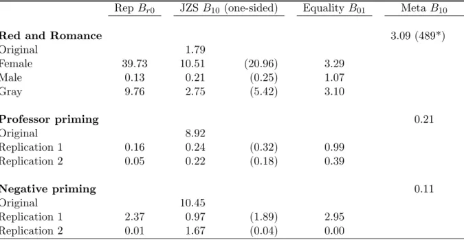
Rep Br0 JZSB10 (one-sided) EqualityB01 MetaB10
Red and Romance 3.09 (489*)
Original 1.79
Female 39.73 10.51 (20.96) 3.29
Male 0.13 0.21 (0.25) 1.07
Gray 9.76 2.75 (5.42) 3.10
Professor priming 0.21
Original 8.92
Replication 1 0.16 0.24 (0.32) 0.99
Replication 2 0.05 0.22 (0.18) 0.39
Negative priming 0.11
Original 10.45
Replication 1 2.37 0.97 (1.89) 2.95
Replication 2 0.01 1.67 (0.04) 0.00
* Result for the meta-analysis without the Male study.
Table 5: Results for four different Bayes factor tests applied to three example studies. Bayes factors higher than 1 favor the hypothesis that an effect is present. Note: “Rep B10” is the new Bayes factor test for replication; “JZS B10” is the two-sided independent default Bayes factor test, with the result of the one-sided test between brackets; “EqualityB01” is the equality-of-effect-size Bayes factor test; and “MetaB10” is the fixed-effect meta-analysis Bayes factor test.
We now re-analyze these results with our Bayesian replication tests, assuming that Experiment 1 from Elliot et al. (2010) is the original study and the others are the replication attempts. The results are summarized in Table 5.7
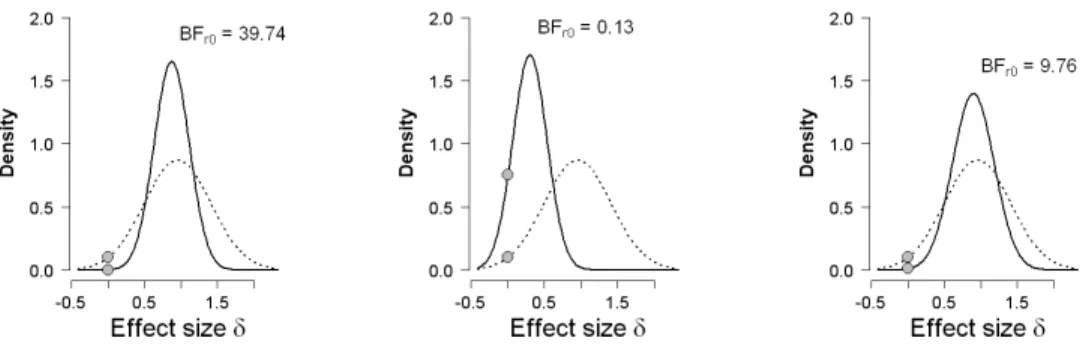
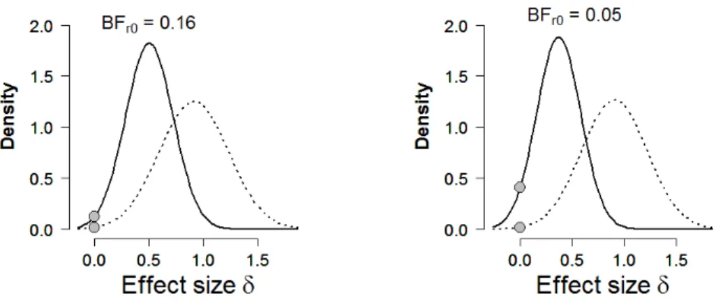
Before discussing the extant Bayes factor tests we first discuss and visualize the results from our new Bayes factor test for replication. The left panel of Figure 2 shows the results for the data from the female students in Elliot et al.’s Experiment 2. The dotted line indicates the prior distribution for the replication test, that is, the proponent’s posterior distribution for effect size after observing the data from the original experiment,p(δ|Yorig). The solid
line indicates the posterior distribution for effect size after observing the additional data from the replication experiment, p(δ |Yrep, Yorig). This posterior distribution assigns more
mass to values ofδ higher than zero than did the prior distribution, a finding that suggests replication success. The extent of this success is quantified by the computation of Br0, which yields 39.73: the data from the female students in Experiment 2 are about 40 times more likely under the proponent’s replication hypothesis Hr than under the skeptic’s null
hypothesis H0.
The outcome of the new Bayesian replication t test is visualized by the ordinates of the prior and posterior distributions at δ = 0, indicated in the left panel of Figure 2 by the two filled circles. Intuitively, the height of the prior distribution at δ = 0 reflects the believability of H0 before seeing the data from the replication attempt, and the height of
7
the posterior distribution at δ = 0 reflects the believability of H0 after seeing those data. In this case, observing the replication data decreases the believability ofH0. It so happens that the ratio of the ordinates exactly equals the Bayes factor Br0 (i.e., the Savage-Dickey density ratio test, see e.g., Dickey & Lientz, 1970; Wagenmakers, Lodewyckx, Kuriyal, & Grasman, 2010), providing a visual confirmation of the test outcome.
The middle panel of Figure 2 shows the results for the data from the male students in Elliot et al.’s Experiment 2. The posterior distribution assigns more mass toδ= 0 than does the prior distribution, indicating evidence in favor of the null hypothesisH0 over the replication hypothesis Hr. The Bayesian replication test yields Br0= 0.13, indicating that the replication data are 1/.13 = 7.69 times more likely underH0 than under Hr.
Finally, the right panel of Figure 2 shows the results for the data from Elliot et al.’s Experiment 3. After observing the data from this replication attempt the posterior distribution assigns more mass to values ofδhigher than zero than did the prior distribution; hence the Bayesian replication test indicates support for the replication hypothesisHrover
the null hypothesis H0. The Bayes factor equals 9.76, indicating that the data are almost 10 times more likely to occur under Hr than under H0. Because the sample size in this replication attempt is smaller than in the first replication attempt, the posterior is less peaked and the test outcome less extreme.
Figure 2. Results from the Bayes factor replication test applied to Experiment 2 and 3 from Elliot et al. (2010). The original experiment had shown that female students judge men in red to be more attractive. The left and middle panel show the results from Elliot et al.’s Experiment 2 (for female and male students, respectively), and the right panel shows the results from Elliot et al.’s Experiment 3 that featured a different control condition. In each panel, the dotted lines represent the posterior from the original experiment, which is used as prior for effect size in the replication tests. The solid lines represent the posterior distributions after the data from the replication attempt are taken into account. The grey dots indicate the ordinates of this prior and posterior at the skeptic’s null hypothesis that the effect size is zero. The ratio of these two ordinates gives the result of the replication test.
In contrast to the analysis above, the three extant Bayes factor tests produce results that are more unequivocal. The default JZS Bayes factor equals 1.79 for the original ex-periment, indicating that the data are uninformative, as they are almost as likely to have occurred under the null hypothesis as under the alternative hypothesis. The study with female students yields strong support in favor of the presence of an effect (B10 = 10.51),
whereas the study with male students yields moderate evidence in favor of the absence of an effect (B01 = 1/B10 = 1/0.21 = 4.76). The study with the gray background, however, yields only anecdotal support for the presence of an effect (B10 = 2.75; a one-sided test, however, almost doubles the support, B10= 5.42).
The equality-of-effect-size Bayes factor test does not yield strong support for or against the hypothesis that the effect sizes are equal, with Bayes factors that never exceed 3.29. The fixed-effect meta-analysis Bayes factor test that pools the data from all four studies yields B10 = 3.09 in favor of the presence of an overall effect. When the experiment with male students is omitted the pooled Bayes factor isB10= 489, indicating extreme evidence in favor of an effect.
Example 2: Dissimilarity Contrast in the Professor Priming Effect
Seminal work by Dijksterhuis and others (e.g., Dijksterhuis & van Knippenberg, 1998; Dijksterhuis et al., 1998) has suggested that priming people with intelligence-related con-cepts (e.g., “professor”) can make them behave more intelligently (e.g., answer more trivial questions correctly). The extent to which this effect manifests itself is thought to depend on whether the prime results in assimilation or contrast (e.g., Mussweiler, 2003). Specifically, the presentation of general categories such as “professor” may lead to assimilation (i.e., activation of the concept of intelligence), whereas the presentation of a specific exemplar such as “Einstein” may lead to contrast (i.e., activation of the concept of stupidity).
However, LeBoeuf and Estes (2004) argued that the balance between assimilation and contrast is determined not primarily by whether the prime is a category or an exemplar, but rather by whether the prime is perceived as relevant in the social comparison process. To test their hypothesis, LeBoeuf and Estes (2004) designed an experiment in which different groups of participants were first presented with either the category prime “professor” or the exemplar prime “Einstein”. To manipulate prime relevance participants were then asked to list similarities and differences between themselves and the presented prime. Subsequently, a test phase featured a series of multiple-choice general knowledge questions.
The results showed that performance was better in the difference-listing condition than in the similarity-listing condition. LeBoeuf and Estes (2004) interpreted these find-ings as follows: “As hypothesized, when participants were encouraged to perceive themselves as unlike a prime, behavior assimilated to prime activated traits, presumably because the prime was rejected as a comparison standard. When participants contemplated how they were similar to a prime, that prime was seemingly adopted as a relevant standard for self-comparison. With the current primes, such a comparison led to negative selfevaluations of intelligence and to lower test performance. Counterintuitively, participants who considered similarities between themselves and an intelligent prime exhibitedworse performance than did participants who considered differences between themselves and an intelligent prime.” (pp. 616-617, italics in original).
Among the various conditions of Experiment 1 in LeBoeuf and Estes (2004), the best performance was attained in the “differences to Einstein” condition (56.2% correct) whereas the worst performance was observed in the “similarities to professors” condition (45.2%), a performance gap that was highly significant (t(42) = 3.00, p =.005, δ =.45 ). These two cells in the design were the target of two recent replication attempts by Shanks et al. (2013). Specifically, Experiment 5 from Shanks et al. (2013) was designed to be
“as close to LeBoeuf and Estes’ study as possible” and yielded a nonsignificant effect that was slightly in the opposite direction (t(47) = −.25, p = .60, δ =−.03, one-sided t test). Experiment 6 from Shanks et al. (2013) tried to maximize the possibility of finding the effect by informing participants beforehand about the hypothesized effects of the primes; however, the results again yielded a nonsignificant effect that was slightly in the opposite direction (t(30) =−1.25,p=.89,δ =−.22, one-sidedt test).
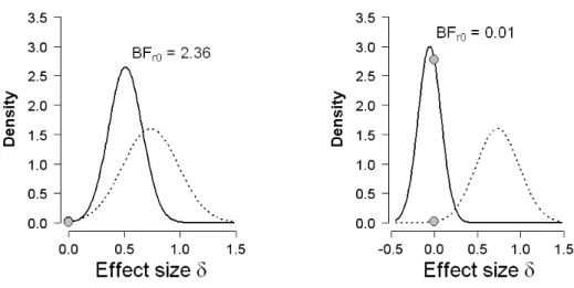
We now re-analyze these results, assuming that Experiment 1 from LeBoeuf and Estes (2004) is the original study and Experiment 5 and 6 from Shanks et al. (2013) are the replication attempts. The resulting Bayes factors are presented in Table 5.
Before discussing the extant Bayes factor tests we first discuss and visualize the results from our new Bayes factor test for replication. In both panels of Figure 3, the dotted line indicates the prior distribution for the replication test, that is, the proponent’s posterior distribution for effect size after observing the data from the original experiment,p(δ |Yorig).
The left panel of Figure 3 shows the results for the data from Shanks et al.’s Experiment 5. The solid line indicates the posterior distribution for effect size after observing the additional data from the replication experiment, p(δ |Yrep, Yorig). The posterior distribution assigns
more mass to δ = 0 than does the prior distribution, indicating evidence in favor of the null hypothesisH0 over the replication hypothesis Hr. The Bayesian replication test yields
Br0 = 0.23, indicating that the replication data are 1/.23 = 4.35 times more likely under H0 than under Hr. This constitutes some evidence against Hr, although it is relatively
weak and only just exceeds Jeffreys’ threshold for evidence that is “not worth more than a bare mention”.
The right panel of Figure 3 shows the results for the data from Shanks et al.’s Exper-iment 6. The solid line again indicates the posterior distribution after observing the data from the replication experiment. As in the left panel, the posterior distribution assigns more mass to δ = 0 than does the prior distribution, and the Bayesian replication test yields Br0 = 0.05, indicating that the replication data are 1/.05 = 20 times more likely underH0 than underHr. This constitutes strong evidence against Hr.
The results from the three extant Bayes factor tests are as follows. The default JZS Bayes factor equals 8.92 for the original experiment, indicating moderate to strong support for the alternative hypothesis. The two replication attempts, however, show the opposite pattern. In both studies, the data are about five times more likely under the null hypothesis than under the alternative hypothesis.
The equality-of-effect-size Bayes factor test does not yield strong support for or against the hypothesis that the effect sizes are equal: for the first replication attempt the outcome is almost completely uninformative, and for the second replication attempt the data are only 2.75 (1/.39) times more likely under the hypothesis that the effect sizes are unequal rather than equal. The fixed-effect meta-analysis Bayes factor test that pools the data from all three studies yields B10 = 0.21 in favor of the presence of an overall effect, which indicates that the combined data are about five times (i.e., 1/.21) more likely under the null hypothesis of no effect.
Example 3: Negative Priming
Negative priming refers to the decrease in performance (e.g., longer response times or RTs, more errors) for a stimulus that was previously presented in a context in which it
Figure 3. Results from the Bayes factor replication test applied to Experiment 5 (left panel) and Experiment 6 (right panel) from Shanks et al. (2013). In each panel, the dotted lines represent the posterior from the original experiment by LeBoeuf and Estes (2004), which is used as prior for effect size in the replication tests. The solid lines represent the posterior distributions after the data from the replication attempt are taken into account. The grey dots indicate the ordinates of this prior and posterior at the skeptic’s null hypothesis that the effect size is zero. The ratio of these two ordinates gives the result of the replication test.
had to be ignored. For instance, assume that on each trial of an experiment, participants are confronted with two words: one printed in red, the other in green. Participants are told to respond only to the red target word (e.g., by indicating whether or not it represents an animate entity, horse: yes, furnace: no) and ignore the green distractor word. Negative priming is said to have occurred when performance on the target word suffers when, on the previous trial, this word same was presented as a green distractor. The theoretical relevance of negative priming is that it is evidence for inhibitory processing – commonly, negative priming is attributed to an attentional mechanism that actively suppresses or inhibits irrelevant stimuli; when these inhibited stimuli later become relevant and need to be re-activated, this process takes time and a performance decrement is observed.
However, the standard suppression account of negative priming was called into ques-tion by Milliken et al. (1998), who showed that negative priming can also be observed in situations where the first presentation of the repeated item does not specifically call for it to be ignored. Specifically, we focus here on Experiment 2A from Milliken et al. (1998), where participants had to name a target word printed in red, while ignoring a distractor word printed in green.
Prior to the target stimulus display, a prime word was presented for 33 ms, printed in white. No action was required related to the prime word. In the unrepeated condition, the prime was not related to the words from the target display; in the repeated condition, the prime was identical to the target word that was presented 500 ms later. Despite the fact that the prime was so briefly presented that most participants were unaware of its presence, and despite the fact that no active suppression of the prime was called for, Milliken et al. (1998) nonetheless found evidence for negative priming: RTs were 8 ms slower in the repeated than
in the unrepeated condition, t(19) = 3.29, p < .004, δ=.74.
The experiment by Milliken et al. (1998) was the target for two nearly exact repli-cation attempts. In Experiment 1A from Neill and Kahan (1999), the negative priming effect was again observed: RTs in the repeated condition were 13 ms slower than those in the unrepeated condition, t(29) = 2.06, p = .048, δ = .38. However, the results from Experiment 1B showed the opposite result, with RTs in the repeated condition being 7 ms faster than those in the unrepeated condition, t(43) =−2.40,p=.021, δ=.37.
We now re-analyze these results with our Bayesian replication t test, assuming that Experiment 2A from Milliken et al. (1998) is the original study and Experiments 1A and 1B from Neill and Kahan (1999) are the replication attempts. The results are presented in Table 5.
Before discussing the extant Bayes factor tests we first discuss and visualize the results from our new Bayes factor test for replication. Similar to the previous examples, in both panels of Figure 4 the dotted line indicates the prior distribution for the replication test, that is, the proponent’s posterior distribution for effect size after observing the data from the original experiment,p(δ|Yorig). The left panel of Figure 4 shows the results for the data
from Neill and Kahan’s Experiment 1A. The solid line indicates the posterior distribution for effect size after observing the additional data from the replication experiment, p(δ | Yrep, Yorig). Although barely discernable from the plot, the posterior distribution assigns
less mass to δ = 0 than does the prior distribution, indicating evidence in favor of the replication hypothesisHr over the null hypothesisH0. The Bayesian replication test yields Br0 = 2.37, indicating that the replication data are 2.37 times more likely under Hr than
under H0. This constitutes evidence in favor of the replication hypothesis Hr, albeit weak
and, according to Jeffreys, “not worth more than a bare mention”.
The right panel of Figure 4 shows the results for the data from Neill and Kahan’s Experiment 1B. The solid line again indicates the posterior distribution after observing the data from the replication experiment. Now the posterior distribution assigns much more mass to δ = 0 than does the prior distribution, and the Bayesian replication test yields Br0 = 0.01, indicating that the replication data are 1/.01 = 100 times more likely under H0 than under Hr. This constitutes compelling evidence againstHr.
The results from the three extant Bayes factor tests are as follows. The default JZS Bayes factor equals 10.45 for the original experiment, indicating strong support for the alternative hypothesis. The results for the two replication attempts, however, are unequiv-ocal. In both studies, the data are about equally likely under the null hypothesis as under the alternative hypothesis. For the second replication attempt, this outcome is artificial, brought about by the fact that the analyses are two-sided instead of one-sided. A one-sided default Bayes factor test for the second replication attempt provides strong evidence in favor of the null hypothesis versus the one-sided alternative hypothesis that postulates a decrease in performance in the repeated condition, B01 = 26.87 (Morey & Wagenmakers, 2014; Wagenmakers et al., 2010).
For the first replication attempt, the equality-of-effect-size Bayes factor test provides anecdotal support for the equality of effect sizes; however, for the second replication attempt the test strongly supports the hypothesis of unequal effect sizes – consistent with the fact that the effect is in the opposite direction. Finally, the fixed-effect meta-analysis Bayes factor test that pools the data from all three studies yields B10 = 0.11 in favor of the
Figure 4. Results from the Bayes factor replication test applied to the replication studies of Neill and Kahan (1999) 1A (left panel) and 1B (right panel). In each panel, the dotted lines represent the posterior from the original experiment by Milliken et al. (1998), which is used as prior for effect size in the replication tests. The solid lines represent the posterior distributions after the data from the replication attempt are taken into account. The grey dots indicate the ordinates of this prior and posterior at the skeptic’s null hypothesis that the effect size is zero. The ratio of these two ordinates gives the result of the replication test.
presence of an overall effect, which indicates that the combined data are about ten times (1/.11) more likely under the null hypothesis of no effect.
Discussion
Inspired by recent work from Simonsohn (2013) and Dienes (2011), we proposed a Bayesian replication test to quantify the extent to which a replication attempt has suc-ceeded or failed. The test assesses the relative adequacy of two hypotheses: the skeptic’s null hypothesis and the proponent’s replication hypothesis. The replication hypothesis is formalized as the posterior distribution on effect size that is obtained from the original experiment.
Our Bayesian replication test has several advantages over existing methods. First, our test summarizes the proponent’s belief by an entire distribution of effect sizes, not just a point estimate; this way, the sample size of the original experiment is fully taken into account. Second, our test does not require the user to specify prior distributions, immunizing it against the popular objection that Bayes factor hypothesis tests are overly sensitive to the choice of prior distributions (Kruschke, 2010; Liu & Aitkin, 2008; but see Vanpaemel, 2010). Third, by taking into account the size of the original effect, the test is optimally sensitive to detect replication effects of the same size as observed in the original study. In addition, there are the general advantages of Bayes factors over classicalpvalue procedures (e.g., Wagenmakers, Lee, Lodewyckx, & Iverson, 2008); for instance, Bayes factors do not assign special status to the null hypothesis, Bayes factors promote quantitative thinking by