Distributed Optimization by Ant Colonies

APPEARED IN PROCEEDINGS OF ECAL91 - EUROPEAN CONFERENCE ON ARTIFICIAL LIFE, PARIS, FRANCE, ELSEVIER PUBLISHING, 134–142.

Distributed Optimization

by Ant Colonies

Alberto Colorni, Marco Dorigo, Vittorio Maniezzo Dipartimento di Elettronica, Politecnico di Milano Piazza Leonardo da Vinci 32, 20133 Milano, Italy

e-mail: [email protected] [email protected]

Abstract

Ants colonies exhibit very interesting behaviours: even if a single ant only has simple ca-pabilities, the behaviour of a whole ant colony is highly structured. This is the result of coordi-nated interactions. But, as communication possibilities among ants are very limited, interac-tions must be based on very simple flows of information. In this paper we explore the implica-tions that the study of ants behaviour can have on problem solving and optimization. We intro-duce a distributed problem solving environment and propose its use to search for a solution to the travelling salesman problem.

1. Introduction

In this paper we propose a novel approach to distributed problem solving and optimization based on the result of low-level interactions among many cooperating simple agents that are not aware of their cooperative behaviour. Our work has been inspired by the study of ant colonies: in these systems each ant performs very simple actions and does not explicitly know what other ants are doing. Nevertheless everybody can observe the resulting highly structured behaviour.

In section 2 we explain the background on which our speculations have been built. We decided to develop a software environment to test our ideas on a very difficult and well known problem: the travelling salesman problem - TSP. We call our system, described in section 3, the ant system and we propose in this paper three possible instantiations to the TSP problem: the ANT-quantity and the ANT-density systems, described in section 4, and the ANT -cycle system, introduced in section 5. Section 6 presents some experiments, together with simulation results and discussion. In section 7 we sketch some conclusions and prefigure the directions along which our research work will proceed in the near future.

2. Motivations

The animal realm exhibits several cases of social systems having poor individual capabilities when compared to their complex collective behaviours. This is observed at different evolution-ary stages, from bacteria [11], to ants [8], caterpillars [5] molluscs and larvae. Moreover, the same causal processes that originate these behaviours are largely conserved in higher level species, like fishes, birds and mammals. These species make use of different communication media, adopted in less ubiquitous situation but essentially leading to the same patterns of be-haviours (see for example the circular mills [3]).

This suggests that the underlying mechanisms have proven evolutionarely extremely effec-tive and are therefore worth of being analyzed when trying to achieve the similar goal of per-forming complex tasks by distributing activities over massively parallel systems composed of computationally simple elements.

One of the better studied natural cases of distributed activities regards ant colonies [2]: we outline here the main features of the models so far proposed to explain ant colonies behaviour. These features have been the basis for the definition of a distributed algorithm, that we have applied to the solution of "difficult" (NP-hard) computational problems.

The problem of interest is how almost blind animals manage to establish shortest route paths from their colony to feeding sources and back.

In the case of ants, the media used to communicate among individuals information regarding paths and used to decide where to go consists of pheromone trails. A moving ant lays some pheromone (in varying quantities) on the ground, thus marking the path it followed by a trail of this substance. While an isolated ant moves essentially at random, an ant encountering a previ-ously laid trail can detect it and decide with high probability to follow it, thus reinforcing the trail with its own pheromone. The collective behaviour that emerges is a form of autocatalytic behaviour — or allelomimesis — where the more are the ants following a trail, the more that trail becomes attractive for being followed. The process is thus characterized by a positive feedback loop, where the probability with which an ant chooses a path increases with the num-ber of ants that chose the same path in the preceding steps.

In Fig.1 we present an example of how allelomimesis can lead to the identification of the shortest path around an obstacle.

A E

Obstacle

B D

H C

A E

Obstacle

B D

C

A E

a) b) c)

Fig.1 - a) Some ants are walking on a path between points A and E b) An obstacle suddenly appears and the ants must get around it c) At steady-state the ants choose the shorter path

The experimental setting is the following: there is a path along which ants are walking (for example it could be a path from a food source A to the nest E - Fig.1a). Suddenly an obstacle appears and the previous path is cut off. So at position B the ants walking from E to A (or at position D those walking in the opposite direction) have to decide whether to turn right or left (Fig.1b). The choice is influenced by the intensity of the pheromone trails left by preceding ants. A higher level of pheromone on the right path gives an ant a stronger stimulus and thus an higher probability to turn right. The first ant reaching point B (or D) has the same probability to turn right or left (as there was no previous pheromone on the two alternative paths). Being path BCD shorter than BGD, the first ant following it will reach D before the first ant following path BGD. The result is that new ants coming from ED will find a stronger trail on path DCB, caused by the half of all the ants that by chance decided to approach the obstacle via ABCD and by the already arrived ones coming via BCD: they will therefore prefer (in probability) path DCB to path DGB. As a consequence, the number of ants following path BCD will be higher,

in the unit of time, than the number of ants following BGD. This causes the quantity of pheromone on the shorter path to grow faster than on the longer one, and therefore the probability with which any single ant chooses the path to follow is quickly biased towards the shorter one. The final result is that very quickly all ants will choose the shorter path (Fig.1c). However, the decision of whether to follow a path or not is never deterministic, thus allowing a continuos exploration of alternative routes.

Computational models have been developed, to simulate the food-searching process [3], [8]. The results are satisfactory, showing that a simple probabilistic model is enough to justify complex and differentiated collective patterns. This is an important result, where a minimal level of individual complexity can explain a complex collective behaviour.

An increase in the computational complexity of each individual, once established the lowest limit needed to account for the desired behaviours, can help in escaping from local optima and to face environmental changes. Trail laying regulated by feedback loop just eases ants to pursue the path followed by the first ant which reached its objective, but that path could easily be suboptimal. If we move from the goal of modeling natural reality to that of designing agents that perform food-seeking in the most efficient possible way, an increase in the individual agent's complexity could direct the search in front of an increment of computational cost. In this case we face the trade-off between individual performance and computational overhead caused by increasing population size: we are interested in the simplest models that take into account efficient shortest route identification and optimization.

3. The Ant system

We introduce in this section our approach to the distributed solution of a difficult problem by many locally interacting simple agents. We call ants the simple interacting agents and ant-al-gorithms the class of alant-al-gorithms we have defined. We first describe the general characteristics of the ant-algorithms and then introduce three of them, called ANT-density, ANT-quantity and ANT-cycle.

As a first test of the ant-algorithms, we decided to apply them to the well-known travelling salesman problem (TSP), to have a comparison with results obtained by other heuristic ap-proaches: the model definition is influenced by the problem structure, however we refer the reader to [1] to see how the same approach can be used to solve related optimization problems.

Given a set of n towns, the TSP problem can be stated as the problem of finding a minimal length closed tour that visit each town once. Let bi(t) (i=1, ..., n) be the number of ants in town iat time t and let

m =

∑

n

be the total number of ants.

Call pathij the shortest path between towns i and j; in the case of euclidean TSP (the one considered in this paper) the length of pathij is the Euclidean distance dij between i and j (i.e. dij=[(x1i-x1

j₎2 _{+ (x} 2 i_-x

2 j₎2_]1/2_).

Let τij(t+1) be the intensity of trail on pathij at time t+1, given by the formula

τij(t+1)=ρ.τij(t)+∆τij(t,t+1) (1)

where

ρ is an evaporation coefficient;

∆τij(t,t+1) =

∑

m

, where ∆τkij(t,t+1) is the quantity per unit of length of trail sub-stance (pheromone in real ants) laid on pathij by the k-th ant between time t and t+1.

The intensity of trail at time 0, τij(0), can be set to arbitrarily chosen values (in our experi-ments a very low value on every pathij).

We call visibility the quantity ηij = 1/dij, and define the transition probability from town ito town j as

pij(t) =

[τij(t)]α⋅[ηij]β [τij(t)]α

∑

j=1 n

⋅[ηij]β (2)

where α and β are parameters that allow a user control on the relative importance of trail versus visibility. Therefore the transition probability is a trade-off between visibility, which says that close towns should be chosen with high probability, and trail intensity, that says that if on pathij there is a lot of traffic then it is highly desirable.

In order to satisfy the constraint that an ant visits n different towns (i.e., it identifies a n-towns cycle), we associate to each ant a data structure, called tabu list1_{, that memorizes the} towns already visited up to time t and forbids the ant to visit them again before a cycle has been completed. When a cycle is completed the tabu list is emptied and the ant is free again to choose its way.

Different choices about how to compute ∆τkij(t,t+1) and when to update the τij(t)cause dif-ferent instantiations of the ant-algorithm. In the next section we present three algorithms we used as experimental test-bed for our ideas. Their names are ANT-density, ANT-quantity and ANT-cycle.

4. The ANT-quantity and ANT-density algorithms

In the ANT-quantity model a constant quantity Q1 of pheromone is left on pathij every time an ant goes from i to j; in the ANT-density model an ant going from i to j leaves Q2 units of pheromone for every unit of length.

Therefore, in the ANT-quantity model

∆τkij(t,t+1)=







dij

if k-th ant goes from i to j between t and t+1 0 otherwise

(3)

and in the ANT-density model we have

∆τkij(t,t+1)=  

 Q2 if k-th ant goes from i to j between t and t+1

0 otherwise (4)

From these definitions it is clear that the increase in pheromone intensity on pathij when an ant goes from i to j is independent of dij in the ANT-density model, while it is inversely pro-1 _{Even though the name chosen recalls tabu search, proposed in [6] and [7], there are substantial differences} between our approach and tabu search algorithms. We mention here (1) the absence of any aspiration function and (2) the difference of the elements recorded in the tabu list: permutations in the case of tabu search, cities in our case.

portional to dij in the ANT-quantity model (i.e. shorter paths are made more desirable by ants in the ANT-quantity model, thus further reinforcing the visibility factor in equation (2) ).

The ANT-density and ANT-quantity algorithms are then 1 Initialize:

Set t:=0

Set an initial value τij(t) for trail intensity on every pathij Place bi(t) ants on every node i

Set ∆τij(t,t+1):= 0 for every i and j

2 Repeat until tabu list is full {this step will be repeated n times} 2.1 For i:=1 to n do {for every town}

For k:=1 to bi(t) do {for every ant on town i at time t}

Choose the town to move to, with probability pij given by equation (2), and move the k-th ant to the chosen location

Insert the chosen town in the tabu list of ant k

Set ∆τij(t,t+1):= ∆τij(t,t+1) + ∆τijk(t,t+1) computing ∆τijk(t,t+1) as defined in (3) or in (4)

2.2 Compute τij(t+1) and pij(t+1)according to equations (1) and (2) 3 Memorize the shortest path found up to now and empty all tabu lists 4 If not(End_Test)

then set t:=t+1

set ∆τij(t,t+1):=0 for every i and j goto step 2

else

print shortest path and Stop

{End_test is currently defined just as a test on the number of cycles}. In words the algorithms work as follows.

At time zero an initialization phase takes place during which ants are positioned on different towns and initial values for trail intensity are set on paths. Then every ant moves from town i to town j choosing the town to move to with a probability that is given as a function (with pa-rameters α and β) of two desirability measures: the first (called trail - τij) gives information about how many ants in the past have chosen that same pathij, the second (called visibility

-ηij) says that the closer a town the more desirable it is (setting α = 0 we obtain a stochastic greedy algorithm with multiple starting points, with α = 0 and β -> ∞ we obtain the standard one).

Each time an ant makes a move, the trail it leaves on pathij is collected and used to compute the new values for path trails. When every ant has moved, trails are used to compute transition probabilities according to formulae (1) and (2).

After n moves the tabu list of each ant will be full: the shortest path found is computed and memorized and tabu lists are emptied. This process is iterated for an user-defined number of cycles.

5. The ANT-cycle algorithm

In the ANT-cycle system we introduced a major difference with respect to the two previous systems. Here ∆τkij is not computed at every step, but after a complete tour (n steps). The value of ∆τk_ij(t,t+n) is given by

∆τijk(t,t+n) =

   Q3

Lk if k-th ant uses pathij in its tour 0 otherwise

(5)

where Q3 is a constant and Lk _{is the tour length of the k-th ant. This corresponds to an} adapta-tion of the ANT-quantity approach, where trails are updated at the end of a whole cycle instead than after each single move.

The value of the trail is also updated every n steps according to a formula very similar to (1)

τij(t+n) = ρ⋅τij(t)+∆τij(t,t+n) (1')

where∆τij(t,t+n) =

∑

m

. The ANT-cycle algorithm is then 1 Initialize:

Set t:=0

Set an initial value τij(t) for trail intensity on every pathij Place bi(t) ants on every node i

Set ∆τij(t,t+n):= 0 for every i and j

2 Repeat until tabu list is full {this step will be repeated n times} 2.1 For i:=1 to n do {for every town}

For k:=1 to bi(t) do {for every ant on town i at time t}

Choose the town to move to, with probability pij given by equation (2), and move the k-th ant to the chosen location

Insert the chosen town in the tabu list of ant k 2.2 Compute ∆τkij(t,t+n) as defined in (5)

2.3 Compute∆τij(t,t+n) =

∑

m

2.4 Compute the new values for τij(t+n) and pij(t+n) according to equations (1') and (2)

3 Memorize the shortest path found up to now and empty all tabu lists 4 If not(End_Test)

then set t:=t+n

set ∆τij(t,t+n):=0 for every i and j goto step 2

else

print shortest path and Stop

6. Computational results

The three reported algorithms have a performance which strongly depends on the parameter setting under which they are run. The parameters are: α (sensibility to trails), β (sensibility to distance), ρ (evaporation rate of pheromone trails) and Qh (algorithm-specific, related to how much pheromone is laid down to form trails). Moreover, we are interested in studying how our algorithms scale up with the increase of the number of the towns in the tour and how the num-ber of ants affects the overall performance.

Since we have not yet developed a mathematical analysis of the models, which would yield the optimal parameter setting in each situation, we ran several simulations, to collect statistical data for this purpose. The results are sketched in the following, for each algorithm.

ANT-quantity and ANT-density

The outcomes of these two models are very similar, except that the ANT-quantity has shown to be slightly more prone to get stuck in local minima (see [1] for a more detailed analysis of their differences).

Simulations run on small-sized problems (10 cities, CCAO problem from [9], see Fig.2) and with initially an ant per city have shown that these two models are very sensible to β, while their behaviour is almost unaffected by trails.

Fig.2 - CCA0 problem and relative optimal tour

We tested several values for each parameter, all the other being constant, over ten simulations for each setting in order to achieve some statistical information about the average evolution. The values tested were: α∈{0, 0.5, 1, 2, 5, 10}, β∈{0, 0.5, 1, 2, 5, 10}, ρ∈{0.5, 0.7, 0.9} and Qh∈{10, 100, 10000}. The results show that for β=0 the algorithms were consistently incapable of finding the optimum, for β=0.5 it took them an average of 12.4 cycles to find it, for every β≥1 the optimum was found in about 3 or 4 cycles. These results hold for each combination of values of α, ρ and Qh. With β=5 or β=10 we noticed an increase in the number of times in which the algorithms found the optimum at the first iteration, but it was not statistically significative (at a level of confidence of 0.05).

Parameters α, ρ and Qh affected the time required to have a uniform behaviour in the ant population (i.e. the same tour followed by every ant). An increase of Qh proved equivalent to an increase of α. Even though in no case we had a complete convergence after having found an optimum, in almost all the cases when the simulation was allowed to go on for some thousands of iterations, the average population tour converged to the best tour and the trail pattern converged to the single tour commonly followed.

Cycles Fig.3 - A 1000 cycles run for the ANT-quantity on the 30 cities problem

(α=2, β=5, ρ=0.7,Q1=100)

More demanding tests were run on problems with 30, 50 and 75 cities, taken from [10] and [4] (the data we used in our experiments can be found also in [12]). The results were consistent with those of the ten cities case: the most important parameter is β, the other ones affect the rate of convergence. Increasing sensibility to trail (or relative trail intensity) results in easing con-vergence, according to the inspiring autocatalytic paradigm. With problems of increasing size, the individuation of the best known solution becomes increasingly more rare; however in all cases the algorithms early individuated good solutions, exploring tours composed primarily of the contextually better edges so far individuated (see fig.3). In Fig.4 we present a typical run of the ANT-density algorithm for the 30 cities problem [10] (parameters: 1 ant per city, α=1, β=5,

ρ=0.7, Q2=100).

Fig.4 - A typical evolution of ANT-density (real length = 424.635; integer length = 421) on the 30 cities problem

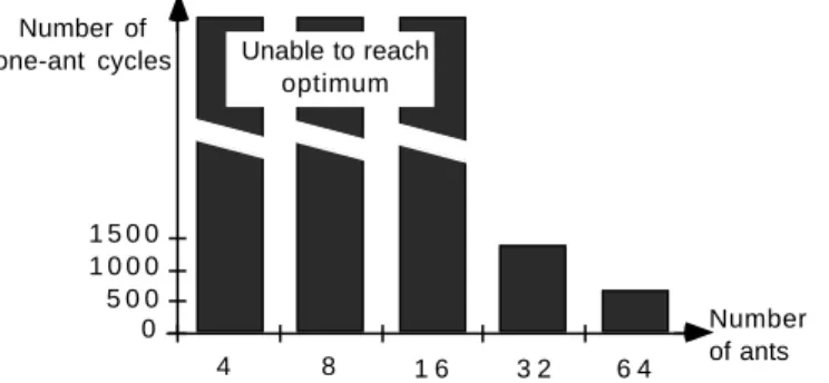
A second set of experiments was run, in order to assess the impact of the number of ants on the efficiency of the solving process. In this case, the test problem involved finding a tour in a 4 by 4 grid of evenly spaced points: this is a problem with a priori known optimal solution (16 if we put to 1 the edge distance of any four evenly neighbouring cities that form a square). In this case we determined the average number of cycles needed in each configuration to reach the optimum, if the optimum could be reached within 200 cycles. In Fig. 5 we present the results obtained for the ANT-density algorithm: on the abscissa there are the total number of ants used in each set of runs, on the ordinate there is the average number of cycles required to reach the optimum, multiplied by the number of ants used (in order to evaluate the efficiency per ant). When the majority of tests with a given configuration could not reach the optimum, we gave an high default value to the corresponding variable.

0 5 0 0 1 0 0 0 1 5 0 0 Number of one-ant cycles

4 8 1 6 3 2 6 4

Number of ants Unable to reach

optimum

Fig.5 - Number of cycles required to reach optimum rated to the total number of ants for the 4x4 grid problem

It can be seen that only configurations with more than an ant per city were able to reach the optimum in less than 200 cycles, and an increase in the number of ants results in an increased efficiency of the overall system.

ANT-cycle

This algorithm performs significantly better than the other two, especially on the harder prob-lems, and is more sensible to variations of parameter values. Problem CCAO, used to roughly determine the sensitivity to each parameter, suggested the following results, changing parameters one at a time with respect to the default configuration α=1, β=1, ρ=0.7, Q3=100:

α: small values of α (<1) lead to slow convergence, the slower the smaller. Moreover for low values of α most of the times only bad solutions can be found. For α≥2 we ob-served an early convergence to suboptimal solutions. The optimal range seems to be 1≤α≤1.5.

β: for β=0 there is no convergence at all, progressively higher values lead to progressively quicker convergence. The behaviour is similar to that observed in the two other models, except that for β >5 the system quickly gets stuck in suboptimal tours.

ρ: values below 0.5 slow down convergence, such as values above 0.8. There seems to be an optimum around 0.7.

Q3: we tested three values, Q3=1, Q3=100 and Q3=10000 but the differences were not significant. Further experimentation is going on.

Experiments run on the 30 cities problem gave results in accordance to those of CCAO: slow or no convergence for β≤1, progressively quicker convergence for increasing betas, too quick for β>5. Values of α in the range [1, 1.5] yield better results than higher or lower values,

ρ≈0.7 is a good value for evaporation, and Q3=100 for the quantity of trail dropped. On this problem ANT-cycle reached the best-known result with a frequency over the number of test runs statistically higher than that of the other two algorithms and, on the whole, identification of good tours seems to be much quicker, even though we devised no index to quantify this. We also found a new optimal tour of length 423.741 (420 with distances rounded to integers; the previous best known tour on the same problem, published in [12] was of integer length 421); see [1] for details.

We tested the algorithm over the Eilon50 and Eilon75 problems [4] on a limited number of runs and with the number of cycles constrained to 3000. Under these restrictions we never got the optimum, but the quick convergence to satisfying solutions was maintained for both the problems (Fig. 6).

Fig. 6 - The new optimal tour obtained with 4200 iterations of ANT-cycle for the 30 cities problem (α=1, β=5, ρ= 0 . 7 , Q3=100).

Real length = 423.741. Integer length = 420.

Fig.7 - A typical evolution of ANT-cycle on the Eilon50 problem (α=1, β=2, ρ=0.7, Q3=100).

Real length = 441.572. Integer length = 438.

Best known solution: integer length = 428.

The tests on the performance with increasing number of ants were conducted with the same modality described for the ANT-density and ANT-quantity systems. The results are shown in Fig.8: it is interesting to note that:

• the algorithm has been consistently able to identify the optimum with any number of ants; • the computational overhead caused by the management of progressively more ants causes the

3/4/94 11

Number of one-ant cycles

Number of ants 0

2 0 0 4 0 0 6 0 0 8 0 0 1 0 0 0 1 2 0 0

4 8 1 6 3 2 6 4

Fig.8 - Number of cycles required to reach optimum rated to the total number of ants for the 4x4 grid problem

7. Conclusions and further work

In this paper we presented a new methodology based on an autocatalytic process and its application to the solution of a classical optimization problem. Simulation results are very en-couraging and we believe the approach can be extended to a broader class of problems. Still a basic questions remains largely with no answer: Why does the ant-algorithm work?

The general idea underlying this model is that of an autocatalytic process pressed by a "greedy force". The autocatalytic process alone tends to converge to a suboptimal path with exponential speed, while the greedy force alone is incapable to find anything but a suboptimal tour. When they work together it looks like the greedy force can give the right suggestions to the autocatalytic process and let it converge on very good, often optimal, solutions very quickly.

We believe that further work can be done along four main research directions:

• the formulation of a mathematical theory of the proposed model and of autocatalytic pro-cesses in general;

• the evaluation of the generality of the approach, through an investigation on which classes of problems can be well solved by this algorithm;

• the study of the implications that our model can have on artificial intelligence, particularly in the pattern recognition and machine learning fields;

• the possibility to exploit the inherent parallelism of the proposed model mapping it on paral-lel architectures.

References

[1] Colorni A., Dorigo M., Maniezzo V.: "An Autocatalytic Optimizing Process", Technical Report n. 91-016 Politecnico di Milano, 1991.

[2] Denebourg J.L., Pasteels J.M., Verhaeghe J.C.: "Probabilistic Behaviour in Ants: a Strategy of Errors?", J. theor. Biol., 105, 1983, pag. 259-271.

3/4/94 12

[3] Denebourg J.L., Goss S.: "Collective patterns and decision-making", Ethology, Ecology & Evolution, 1, 1989, pag. 295-311.

[4] Eilon S., Watson-Gandy T.H.., Christofides N.: "Distribution management: mathematical modeling and prcatical analysis", Operational Research Quarterly, 20, 1969.

[5] Fitzgerald T.D., Peterson S.C.: "Cooperative foraging and communication in caterpil-lars", Bioscience, 38, 1988, pag. 20-25.

[6] Glover F.: "Tabu Search — Part I", ORSA Jou. on Computing, 1, 1989. [7] Glover F.: "Tabu Search — Part II", ORSA Jou. on Computing, 2, 1990.

[8] Goss S., Beckers R., Deneubourg J.L., Aron S., Pasteels J.M.: "How Trail Laying and Trail Following Can Solve Foraging Problems for Ant Colonies", in Hughes R.N. (ed.), NATO ASI Series, Vol. G 20, Behavioural Mechanisms of Food Selection, Springer-Verlag, Berlin, 1990.

[9] Golden B., Stewart W.: "Empiric analysis of heuristics", in Lawler E.L., Lenstra J.K., Rinnooy-Kan A.H.G., Shmoys D.B.: "The Travelling Salesman Problem", Wiley, 1985, pag. 228.

[10] Lin S., Kernighan B.W.: "An effective Heuristic Algorithm for the TSP", Operations re-search, 21, 1973.

[11] Shapiro J.A.: "Bacteria as multicellular organisms", Scientific American, 1988, pag. 82-89.

[12] Whitley D., Starkweather T., Fuquay D.: "Scheduling Problems and Travelling Salesmen: the Genetic Edge Recombination Operator", Proc. of the Third Int. Conf. on Genetic Algorithms, Morgan Kaufmann, 1989.