B
R
ICS
R
S
-01-23
Dan
v
y
&
Nielsen
:
Defu
n
ction
alization
a
t
W
ork
BRICS
Basic Research in Computer Science
Defunctionalization at Work
Olivier Danvy
Lasse R. Nielsen
Copyright c
2001,
Olivier Danvy & Lasse R. Nielsen.
BRICS, Department of Computer Science
University of Aarhus. All rights reserved.
Reproduction of all or part of this work
is permitted for educational or research use
on condition that this copyright notice is
included in any copy.
See back inner page for a list of recent BRICS Report Series publications.
Copies may be obtained by contacting:
BRICS
Department of Computer Science
University of Aarhus
Ny Munkegade, building 540
DK–8000 Aarhus C
Denmark
Telephone: +45 8942 3360
Telefax:
+45 8942 3255
Internet:
[email protected]
BRICS publications are in general accessible through the World Wide
Web and anonymous FTP through these URLs:
http://www.brics.dk
ftp://ftp.brics.dk
Defunctionalization at Work
∗
Olivier Danvy and Lasse R. Nielsen
BRICS
†Department of Computer Science
University of Aarhus
‡June, 2001
Abstract
Reynolds’s defunctionalization technique is a whole-program transfor-mation from higher-order to first-order functional programs. We study practical applications of this transformation and uncover new connec-tions between seemingly unrelated higher-order and first-order specifica-tions and between their correctness proofs. Defunctionalization therefore appears both as a springboard for revealing new connections and as a bridge for transferring existing results between the first-order world and the higher-order world.
∗Extended version of an article to appear in the proceedings of PPDP 2001, Firenze, Italy. †Basic Research in Computer Science (www.brics.dk),
funded by the Danish National Research Foundation.
‡Ny Munkegade, Building 540, DK-8000 Aarhus C, Denmark
Contents
1 Background and Introduction 4
1.1 A sample higher-order program with a static number of closures 4
1.2 A sample higher-order program with a dynamic number of closures 5
1.3 Defunctionalization in a nutshell . . . 7
1.4 Related work . . . 7
1.5 This work . . . 7
2 Defunctionalization of List- and of Tree-Processing Programs 9 2.1 Flattening a binary tree into a list . . . 9
2.2 Higher-order representations of lists . . . 10
2.3 Defunctionalizing Church-encoded non-recursive data structures . 13 2.4 Defunctionalizing Church-encoded recursive data structures . . . 15
2.5 Church-encoding the result of defunctionalization . . . 16
2.6 Summary and conclusion . . . 17
3 Defunctionalization of CPS-Transformed First-Order Programs 17 3.1 String parsing . . . 17
3.2 Continuation-based program transformation strategies . . . 20
3.3 Summary and conclusion . . . 20
4 Two Syntactic Theories in the Light of Defunctionalization 20 4.1 Arithmetic expressions . . . 20
4.1.1 A syntactic theory for arithmetic expressions . . . 21
4.1.2 Implementation . . . 21
4.1.3 Refunctionalization . . . 22
4.1.4 Back to direct style . . . 23
4.2 The call-by-valueλ-calculus . . . 24
4.2.1 A syntactic theory for the call-by-valueλ-calculus . . . . 24
4.2.2 Implementation . . . 24
4.2.3 Refunctionalization . . . 25
4.2.4 Back to direct style . . . 26
4.3 Summary and conclusion . . . 27
5 A Comparison between Correctness Proofs before and after Defunctionalization: Matching Regular Expressions 28 5.1 Regular expressions . . . 28
5.2 The two matchers . . . 29
5.2.1 The higher-order matcher . . . 29
5.2.2 The first-order matcher . . . 30
5.3 The two correctness proofs . . . 30
5.3.1 Correctness proof of the higher-order matcher . . . 32
5.3.2 Correctness proof of the first-order matcher . . . 32
5.4 Comparison between the two correctness proofs . . . 33
6 Conclusions and Issues 35
A Correctness Proof of the Higher-Order Matcher 36
B Correctness Proof of the First-Order Matcher 39
List of Figures
1 Higher-order, continuation-based matcher for regular expressions 29 2 First-order, stack-based matcher for regular expressions . . . 31
1
Background and Introduction
In first-order programs, all functions are named and each call refers to the callee by its name. In higher-order programs, functions may be anonymous, passed as arguments, and returned as results. As Strachey put it [50], functions are second-classdenotable values in a first-order program, andfirst-classexpressible values in a higher-order program. One may then wonder how first-class functions are represented at run time.
• First-class functions are often represented withclosures, i.e., expressible values pairing a code pointer and the denotable values of the variables occurring free in that code, as proposed by Landin in the mid-1960’s [30]. Today, closures are the most common representation of first-class functions in the world of eager functional programming [1, 17, 32], as well as a standard representation for implementing object-oriented programs [23]. They are also used to implement higher-order logic programming [8].
• Alternatively, higher-order programs can be defunctionalized into first-order programs, as proposed by Reynolds in the early 1970’s [43]. In a defunctionalized program, class functions are represented with first-order data types: a first-class function is introduced with a constructor holding the values of the free variables of a function abstraction, and it is eliminated with a case expression dispatching over the corresponding constructors.
• First-class functions can also be dealt with by translating functional pro-grams intocombinatorsand using graph reduction, as proposed by Turner in the mid-1970’s [52]. This implementation technique has been investi-gated extensively in the world of lazy functional programming [27, 29, 37, 38].
Compared to closure conversion and to combinator conversion, defunctional-ization has been used very little. The goal of this article is to study practical applications of it.
We first illustrate defunctionalization with two concrete examples (Sections 1.1 and 1.2). In the first program, two function abstractions are instantiated once, and in the second program, one function abstraction is instantiated re-peatedly. We then characterize defunctionalization in a nutshell (Section 1.3) before reviewing related work (Section 1.4). Finally, we raise questions to which defunctionalization provides answers (Section 1.5).
1.1 A sample higher-order program with a static number of closures
In the following ML program,auxis passed a first-class function, applies it to 1
and 10, and sums the results. Themain function callsauxtwice and multiplies
(* aux : (int -> int) -> int *) fun aux f
= f 1 + f 10
(* main : int * int * bool -> int *) fun main (x, y, b)
= aux (fn z => x + z) *
aux (fn z => if b then y + z else y - z)
Defunctionalizing this program amounts to defining a data type with two con-structors, one for each function abstraction, and its associated apply function. The first function abstraction contains one free variable (x, of type integer), and
therefore the first data-type constructor requires an integer. The second func-tion abstracfunc-tion contains two free variables (y, of type integer, andb, of type boolean), and therefore the second data-type constructor requires an integer and a boolean.
In main, the first first-class function is thus introduced with the first con-structor and the value ofx, and the second with the second constructor and the values ofyandb.
In aux, the functional argument is passed to a second-class function apply
that eliminates it with a case expression dispatching over the two constructors.
datatype lam = LAM1 of int | LAM2 of int * bool (* apply : lam * int -> int *) fun apply (LAM1 x, z)
= x + z
| apply (LAM2 (y, b), z) = if b then y + z else y - z (* aux_def : lam -> int *) fun aux_def f
= apply (f, 1) + apply (f, 10)
(* main_def : int * int * bool -> int *) fun main_def (x, y, b)
= aux_def (LAM1 x) * aux_def (LAM2 (y, b))
1.2 A sample higher-order program with a dynamic number of
clo-sures
A PPDP reviewer wondered what happens for programs that “dynamically gen-erate” new closures, and whether such programs lead to new constants and thus require extensible case expressions. The following example illustrates such a situation and shows that no new constants and no extensible case expressions are needed.
In the following ML program,auxis passed two arguments and applies one to the other. Themainfunction is given a numberiand a list of numbers[j1, j2, ...] and returns the list of numbers[i+j1, i+j2, ...]. One function abstrac-tion,fn i => i + j, occurs in this program, inmain, as the second argument of
aux. Given an input list of lengthn, the function abstraction is instantiatedn times in the course of the computation.
(* aux : int * (int -> int) -> int *) fun aux (i, f)
= f i
(* main = fn : int * int list -> int list *) fun main (i, js)
= let fun walk nil = nil
| walk (j :: js)
= (aux (i, fn i => i + j)) :: (walk js) in walk js
end
Defunctionalizing this program amounts to defining a data type with only one constructor, since there is only one function abstraction, and its associated apply function. The function abstraction contains one free variable (j, of type integer), and therefore the data-type constructor requires an integer.
Inmain, the first-class function is introduced with the constructor and the value ofj.
In aux, the functional argument is passed to a second-class function apply
that eliminates it with a case expression dispatching over the constructor.
datatype lam = LAM of int (* apply : lam * int -> int *) fun apply (LAM j, i)
= i + j
(* aux_def : int * lam -> int *) fun aux_def (i, f)
= apply (f, i)
(* main_def : int * int list -> int list *) fun main_def (i, js)
= let fun walk nil = nil
| walk (j :: js)
= (aux_def (i, LAM j)) :: (walk js) in walk js
end
Given an input list of lengthn, the constructorLAMis usedntimes in the course of the computation.
1.3 Defunctionalization in a nutshell
In a higher-order program, first-class functions arise as instances of function abstractions. All these function abstractions can be enumerated in a whole program. Defunctionalization is thus a whole-program transformation where function types are replaced by an enumeration of the function abstractions in this program.
Defunctionalization therefore takes its roots in type theory. Indeed, a func-tion type hides typing assumpfunc-tions from the context, and, as pointed out by Minamide, Morrisett, and Harper in their work on typed closure conversion [32], making these assumptions explicit requires an existential type. For a whole pro-gram, this existential type can be represented with a finite sum together with the corresponding injections and case dispatch, and this representation is precisely what defunctionalization achieves.
These type-theoretical roots do not make defunctionalization a straitjacket, to paraphrase Reynolds about Algol [42]. For example, one can use several apply functions, e.g., grouped by types, as in Bell, Bellegarde, and Hook’s work [4]. One can also defunctionalize a program selectively, e.g., only its cont-inuations, as in Section 3. One can even envision a lightweight defunction-alization similar to Steckler and Wand’s lightweight closure conversion [48], as in Banerjee, Heintze, and Riecke’s recent work [2].
1.4 Related work
Originally, Reynolds devised defunctionalization to transform a higher-order interpreter into a first-order one [43]. He presented it as a programming tech-nique, and never used it again [44], save for deriving a first-order semantics in his textbook on programming language [45, Section 12.4].
Since then, defunctionalization has not been used much, though when it has, it was as a full-fledged implementation technique: Bondorf uses it to make higher-order programs amenable to first-order partial evaluation [5]; Tolmach and Oliva use it to compile ML programs into Ada [51]; Fegaras uses it in his object-oriented database management system, lambda-DB [18]; Wang and Appel use it in type-safe garbage collectors [55]; and defunctionalization is an integral part of MLton [7] and of Boquist’s Haskell compiler [6].
Only lately has defunctionalization been formalized: Bell, Bellegarde, and Hook showed that it preserves types [4]; Nielsen proved its partial correctness using denotational semantics [35, 36]; and Banerjee, Heintze and Riecke proved its total correctness using operational semantics [2].
1.5 This work
Functional programming encourages fold-like recursive descents, typically using auxiliary recursive functions. Often, these auxiliary functions are higher order in that their co-domain is a function space. For example, if an auxiliary function has an accumulator of typeα, its co-domain isα→β, for someβ. For another example, if an auxiliary function has a continuation of typeα→β, for someβ,
its co-domain is (α→β)→β. How do these functional programs compare to programs written using a first-order, data-structure oriented approach?
Wand’s classical work on continuation-based program transformations [54] was motivated by the question “What is a data-structure continuation?”. Each of the examples considered in Wand’s paper required a eureka step to design a data structure for representing a continuation. Are such eureka steps always necessary?
Continuations are variously presented as a functional representation of the rest of the computation and as a functional representation of the context of a computation [20]. Wand’s work addressed the former view, so let us consider the latter one. For example, in his PhD thesis [19], Felleisen developed a syntactic approach to semantics relying on the first-order notions of ‘evaluation context’ and of ‘plugging expressions into contexts’. How do these first-order notions compare to the notion of continuation?
In the rest of this article, we show that defunctionalization provides a single answer to all these questions. All the programs we consider perform a recur-sive descent and use an auxiliary function. When this auxiliary function is higher-order, defunctionalization yields a first-order version with an accumula-tor (e.g., tree flattening in Section 2.1 and list reversal in Section 2.2). When this auxiliary function is first-order, we transform it into continuation-passing style; defunctionalization then yields an iterative first-order version with an ac-cumulator in the form of a data structure (e.g., string parsing in Section 3.1 and regular-expression matching in Section 5). We also consider interpreters for two syntactic theories and we identify that they are written in a defunction-alized form. We then “refunctionalize” them and obtain continuation-passing interpreters whose continuations represent the evaluation contexts of the corre-sponding syntactic theory (Section 4).
In addition, we observe that defunctionalization and Church encoding have dual purposes, since Church encoding is a classical way to represent data struc-tures with higher-order functions. What is the result of defunctionalizing a
Church-encoded data structure? And what does one obtain when
Church-encoding the result of defunctionalization?
Similarly, we observe that backtracking is variously implemented in a first-order setting with one or two stacks, and in a higher-first-order setting with one or two continuations. It is natural enough to wonder what is the result of Church-encoding the stacks and of defunctionalizing the continuations. One can wonder as well about the correctness proofs of these programs—how do they compare? In the rest of this article, we also answer these questions. We defunctionalize two programs using Hughes’s higher-order representation of intermediate lists and obtain two efficient and traditional first-order programs (Section 2.2). We also clarify the extent to which Church encoding and defunctionalization can be considered as inverses of each other (Sections 2.3, 2.4, and 2.5). Finally, we compare and contrast a regular-expression matcher and its proof before and after defunctionalization (Section 5).
2
Defunctionalization of List- and of Tree-Processing
Pro-grams
We consider several canonical higher-order programs over lists and trees and we defunctionalize them. In each case, defunctionalization yields a known, but unrelated solution. We then turn to Church encoding, which provides a uni-form higher-order representation of data structures. We consider the result of defunctionalizing Church-encoded data structures, and we consider the result of Church-encoding the result of defunctionalization.
2.1 Flattening a binary tree into a list
To flatten a binary tree into a list of its leaves, we choose to map a leaf to a curried list constructor and a node to function composition, homomorphically. In other words, we map a list into the monoid of functions from lists to lists. This definition hinges on the built-in associativity of function composition.
datatype ’a bt = LEAF of ’a
| NODE of ’a bt * ’a bt (* cons : ’a -> ’a list -> ’a list *) fun cons x xs
= x :: xs
(* flatten : ’a bt -> ’a list *) (* walk : ’a bt -> ’a list -> ’a list *) fun flatten t
= let fun walk (LEAF x) = cons x
| walk (NODE (t1, t2)) = (walk t1) o (walk t2) in walk t nil
end
Eta-expanding the result ofwalkand inliningconsandoyields a curried version of the fast flatten function with an accumulator.
(* flatten_ee : ’a bt -> ’a list *) (* walk : ’a bt -> ’a list -> ’a list *) fun flatten_ee t
= let fun walk (LEAF x) a = x :: a
| walk (NODE (t1, t2)) a = walk t1 (walk t2 a) in walk t nil
end
It is also instructive to defunctionalizeflatten. Two functional values occur— one for the leaves and one for the nodes—and therefore they give rise to a data
type with two constructors. Sinceflatten is homomorphic, the new data type is isomorphic to the data type of binary trees, and therefore the associated apply function could be made to work directly on the input tree, e.g., using deforestation [53]. At any rate, we recognize this apply function as an uncurried version of the fast flatten function with an accumulator.
datatype ’a lam = LAM1 of ’a | LAM2 of ’a lam * ’a lam (* apply : ’a lam * ’a list -> ’a list *)
fun apply (LAM1 x, xs) = x :: xs
| apply (LAM2 (f1, f2), xs) = apply (f1, apply (f2, xs)) (* cons_def : ’a -> ’a lam *) fun cons_def x
= LAM1 x
(* o_def : ’a lam * ’a lam -> ’a lam *) fun o_def (f1, f2)
= LAM2 (f1, f2)
(* flatten_def : ’a bt -> ’a list *) (* walk : ’a bt -> ’a lam *) fun flatten_def t
= let fun walk (LEAF x) = cons_def x
| walk (NODE (t1, t2)) = o_def (walk t1, walk t2) in apply (walk t, nil)
end
The monoid of functions from lists to lists corresponds to Hughes’s novel representations of lists [28], which we treat next.
2.2 Higher-order representations of lists
In the mid-1980’s, Hughes proposed to represent intermediate lists as partially applied concatenation functions [28], so that instead of constructing a list xs, one instantiates the function abstractionfn ys => xs @ ys. The key property of this higher-order representation is that lists can be concatenated in constant time. Therefore, the following naive version ofreverse operates in linear time instead of in quadratic time, as with the usual linked representation of lists, where lists are concatenated in linear time.
(* append : ’a list -> ’a list -> ’a list *) fun append xs ys
(* reverse : ’a list -> ’a list *) fun reverse xs
= let fun walk nil = append nil | walk (x :: xs)
= (walk xs) o (append [x]) in walk xs nil
end
Let us defunctionalize this program. First, like Hughes, we recognize that appending the empty list is the identity function and that appending a single element amounts to consing it.
(* id : ’a list -> ’a list *) fun id ys
= ys
(* cons : ’a -> ’a list -> ’a list *) fun cons x xs
= x :: xs
(* reverse : ’a list -> ’a list *) (* walk : ’a list -> ’a list -> ’a list *) fun reverse xs
= let fun walk nil = id
| walk (x :: xs)
= (walk xs) o (cons x) in walk xs nil
end
The function space’a list -> ’a listarises because of three functional values:
id, in one conditional branch; and, in the other, the results of consing an element
and of callingwalk.
We thus defunctionalize the program using a data type with three construc-tors and its associated apply function.
datatype ’a lam = LAM0 | LAM1 of ’a
| LAM2 of ’a lam * ’a lam (* apply : ’a lam * ’a list -> ’a list *) fun apply (LAM0, ys)
= ys
| apply (LAM1 x, ys) = x :: ys
| apply (LAM2 (f, g), ys) = apply (f, apply (g, ys))
This data type makes it plain that in Hughes’s monoid of intermediate lists, concatenation is performed in constant time (here withLAM2).
The rest of the defunctionalized program reads as follows.
(* id_def : ’a lam *) val id_def = LAM0
(* cons_def : ’a -> ’a lam *) fun cons_def x = LAM1 x
(* o_def : ’a lam * ’a lam -> ’a lam *) fun o_def (f, g) = LAM2 (f, g)
(* reverse_def : ’a list -> ’a list *) (* walk : ’a list -> ’a lam *) fun reverse_def xs
= let fun walk nil = id_def | walk (x :: xs)
= o_def (walk xs, cons_def x) in apply (walk xs, nil)
end
The auxiliary functions are only aliases for the data-type constructors. We also observe thatLAM1andLAM2are always used in connection with each other.
Therefore, they can be fused in a single constructorLAM3and so can their
treat-ment inapply lam. The result reads as follows.
datatype ’a lam_alt = LAM0
| LAM3 of ’a lam_alt * ’a
(* apply_lam_alt : ’a lam_alt * ’a list -> ’a list *) fun apply_lam_alt (LAM0, ys)
= ys
| apply_lam_alt (LAM3 (f, x), ys) = apply_lam_alt (f, x :: ys)
(* reverse_def_alt : ’a list -> ’a list *) (* walk : ’a list -> ’a lam_alt *) fun reverse_def_alt xs
= let fun walk nil = LAM0
| walk (x :: xs) = LAM3 (walk xs, x) in apply_lam_alt (walk xs, nil) end
As in Section 2.1, we can see thatreverse def altembeds its input list into the data typelam alt, homomorphically. The associated apply function could there-fore be made to work directly on the input list. We also recognizeapply lam alt
Hughes also uses his representation of intermediate lists to define a ‘fields’ function that extracts words from strings. His representation gives rise to an efficient implementation of the fields function. And indeed, as for reverse above, defunctionalizing this implementation gives the fast implementation that accu-mulates words in reverse order and reverses them using a fast reverse function once the whole word has been found. Defunctionalization thus confirms the effectiveness of Hughes’s representation.
2.3 Defunctionalizing Church-encoded non-recursive data structures
Church-encoding a value amounts to representing it by aλ-term in such a way that operations on this value are carried out by applying the representation to specificλ-terms [3, 9, 24, 33].
A data structure is a sum in a domain. (When the data structure is induc-tive, the domain is recursive.) A sum is defined by its corresponding injection functions and a case dispatch [56, page 133]. Church-encoding a data structure consists in (1) combining injection functions and case dispatch intoλ-terms and (2) operating by function application.
In the rest of this section, for simplicity, we only consider Church-encoded data structures that are uncurried. This way, we can defunctionalize them as a whole.
For example, monotyped Church pairs and their selectors are defined as follows.
(* Church_pair : ’a * ’a -> (’a * ’a -> ’a) -> ’a *) fun Church_pair (x1, x2)
= fn s : ’a * ’a -> ’a => s (x1, x2)
(* Church_fst : ((’a * ’a -> ’a) -> ’b) -> ’b *) fun Church_fst p
= p (fn (x1, x2) => x1)
(* Church_snd : ((’a * ’a -> ’a) -> ’b) -> ’b *) fun Church_snd p
= p (fn (x1, x2) => x2)
A pair is represented as aλ-term expecting one argument. This argument is a selector corresponding to the first or the second projection.
In general, each of the injection functions defining a data structure has the following form.
inji=λ(x1, ..., xn).λ(s1, ..., sm).si(x1, ..., xn)
So what happens if one defunctionalizes a Church-encoded data structure, i.e., the result of the injection functions? Each injection function gives rise to a data-type constructor whose arguments correspond to the free variables in the term underlined just above. These free variables are precisely the parameters
of the injection functions, which are themselves the parameters of the original constructors that were Church encoded.
Therefore defunctionalizing Church-encoded data structures (i.e., the result of their injection functions) gives rise to the same data structures, prior to Church encoding. These data structures are accessed through the auxiliary apply functions introduced by defunctionalization.
For example, monotyped Church pairs and their selectors are defunctional-ized as follows.
• The selectors are closed terms and therefore the corresponding construc-tors are parameterless. By definition, a selector is passed a tuple of argu-ments and returns one of them.
datatype sel = FST | SND
(* apply_sel : sel * (’a * ’a) -> ’a *) fun apply_sel (FST, (x1, x2))
= x1
| apply_sel (SND, (x1, x2)) = x2
• There is one injection function for pairs, and therefore it gives rise to a data type with one constructor for the values of the two free variables of the result ofChurch pair. The corresponding apply function performs a selection. (N.B: apply paircalls apply sel, reflecting the curried type of
Church pair.)
datatype ’a pair = PAIR of ’a * ’a (* apply_pair : ’a pair * sel -> ’a *) fun apply_pair (PAIR (x1, x2), s)
= apply_sel (s, (x1, x2))
• Finally, constructing a pair amounts to constructing a pair, `a la Tarski one could say [21], and selecting a component of a pair is achieved by calling
apply pair, which in turns callsapply sel.
(* Church_pair_def : ’a * ’a -> ’a pair *) fun Church_pair_def (x1, x2)
= PAIR (x1, x2)
(* Church_fst_def : ’a pair -> ’a *) fun Church_fst_def p
= apply_pair (p, FST)
(* Church_snd_def : ’a pair -> ’a *) fun Church_snd_def p
An optimizing compiler would inline both apply functions. The resulting selec-tors, together with the defunctionalized pair constructor, would then coincide with the original definition of pairs, prior to Church encoding.
2.4 Defunctionalizing Church-encoded recursive data structures
Let us briefly consider Church-encoded binary trees. Two injection functions occur: one for the leaves, and one for the nodes. A Church-encoded tree is aλ -term expecting two arguments. These arguments are the selectors corresponding to whether the tree is a leaf or whether it is a node.
fun Church_leaf x
= fn (s1, s2) => s1 x fun Church_node (t1, t2)
= fn (s1, s2) => s2 (t1 (s1, s2), t2 (s1, s2))
Due to the inductive nature of binary trees,Church-nodepropagates the selectors to the subtrees.
In general, each of the injection functions defining a data structure has the following form.
inji=λ(x1, ..., xn).λ(s1, ..., sm).si(x1, ..., xj(s1, ..., sm), ..., xn)
wherexj(s1, ..., sm) occurs for eachxj that is in the data type.
So what happens if one defunctionalizes a Church-encoded recursive data structure, i.e., the result of the injection functions? Again, each injection func-tion gives rise to a data-type constructor whose arguments correspond to the free variables in the term underlined just above. These free variables are precisely the parameters of the injection functions, which are themselves the parameters of the original constructors that were Church encoded.
Therefore defunctionalizing Church-encoded recursive data structures (i.e., the result of their injection functions) also gives rise to the same data struc-tures, prior to Church encoding. These data structures are accessed through the auxiliary apply functions introduced by defunctionalization.
Let us get back to Church-encoded binary trees. Since defunctionalization is a whole-program transformation, we consider a whole program. Let us con-sider the function computing the depth of a Church-encoded binary tree. This function passes two selectors to its argument. The first is the constant function returning 0, and accounting for the depth of a leaf. The second is a function that will be applied to the depth of the subtrees of each node, and computes the depth of the node by taking the max of the depths of the two subtrees and adding one.
fun Church_depth t = t (fn x => 0,
This whole program is defunctionalized as follows.
• The selectors give rise to two constructors,SEL LEAFandSEL NODE, and the corresponding two apply functions,apply sel leafandapply sel node.
datatype sel_leaf = SEL_LEAF fun apply_sel_leaf (SEL_LEAF, x)
= 0
datatype sel_node = SEL_NODE
fun apply_sel_node (SEL_NODE, (d1, d2)) = Int.max (d1, d2) + 1
• As for the injection functions, as noted above, they give rise to two con-structors,LEAFandNODE, and the corresponding apply function.
datatype ’a tree = LEAF of ’a
| NODE of ’a tree * ’a tree fun Church_leaf_def x
= LEAF x
fun Church_node_def (t1, t2) = NODE (t1, t2)
• Finally, the defunctionalized main function applies its argument to the two selectors.
(* depth_def : ’a tree -> int *) (* apply_tree : ’a tree * (sel_leaf * sel_node) -> int *) fun depth_def t
= apply_tree (t, (SEL_LEAF, SEL_NODE)) and apply_tree (LEAF x, (sel_leaf, sel_node))
= apply_sel_leaf (sel_leaf, x)
| apply_tree (NODE (t1, t2), (sel_leaf, sel_node))
= apply_sel_node (sel_node, (apply_tree (t1, (sel_leaf, sel_node)), apply_tree (t2, (sel_leaf, sel_node))))
Again, an optimizing compiler would inline both apply functions andSEL LEAF
and SEL NODE would then disappear. The result would thus coincide with the original definition of binary trees, prior to Church encoding.
2.5 Church-encoding the result of defunctionalization
As can be easily verified with the Church pairs and the Church trees above, Church-encoding the result of defunctionalizing a Church-encoded data struc-ture gives back this Church-encoded data strucstruc-ture: the apply functions revert
to simple applications, the main data-structure constructors become injection functions, and the auxiliary data-structure constructors become selectors.
In practice, however, one often inlines selectors during Church encoding if they only occur once—which Shivers refers to as “super-beta” [46]. Doing so yields an actual inverse to defunctionalization, as illustrated in Sections 4.1.3 and 4.2.3. This “refunctionalization” is also used, e.g., in Danvy, Grobauer, and Rhiger’s work on goal-directed evaluation [13].
In Church-encoded data structures, selectors have the flavor of a continua-tion. In Section 3, we consider how to defunctionalize continuations.
2.6 Summary and conclusion
We have considered a variety of typical higher-order programs and have de-functionalized them. The resulting programs provide a first-order view that reveals the effect of higher-orderness in functional programming. For example, returning a function of type α → β often naturally provides a way to write this function with anα-typed accumulator. For another example, defunction-alizing uncurried Church-encoded data structures leads one back to these data structures prior Church encoding, illustrating that Church encoding and de-functionalization transform data flow into control flow and vice-versa.
3
Defunctionalization of CPS-Transformed First-Order
Pro-grams
As functional representations of control, continuations provide a natural target for defunctionalization. In this section, we investigate the process of transform-ing direct-style programs into continuation-passtransform-ing style (CPS) programs [12, 49] and defunctionalizing their continuation. We then compare this process with Wand’s continuation-based program-transformation strategies [54].
3.1 String parsing
We consider a recognizer for the language {0n1n | n ∈ N}. We write it as a function of type int list -> bool. The input is a list of integers, and the
recognizer checks whether it is the concatenation of a list ofn0’s and of a list ofn1’s, for somen.
We start with a recursive-descent parser traversing the input list.
(* rec0 : int list -> bool *) (* walk : int list -> int list *) fun rec0 xs
= let exception NOT fun walk (0 :: xs’)
= (case walk xs’ of 1 :: xs’’
=> xs’’ | _
=> raise NOT) | walk xs
= xs
in (walk xs = nil) handle NOT => false end
The auxiliary function walk traverses the input list. Every time it encounters
0, it calls itself recursively. When it meets something else than0, it returns the rest of the list, and expects to find1at every return. In case of mismatch (i.e., a list element other than1for returns, or a list that is too short or too long), an exception is raised.
Let us writewalk in continuation-passing style [12, 49]. (* rec1 : int list -> bool *) (* walk : int list * (int list -> bool) -> bool *) fun rec1 xs
= let fun walk (0 :: xs’, k)
= walk (xs’, fn (1 :: xs’’) => k xs’’ | _
=> false) | walk (xs, k)
= k xs
in walk (xs, fn xs’ => xs’ = nil) end
The auxiliary function walk traverses the input list tail-recursively (and thus does not need any exception). If it meets something else than0, it sends the current list to the current continuation. If it encounters0, it iterates down the
list with a new continuation. If the new continuation is sent a list starting with
1, it sends the tail of that list to the current continuation; otherwise, it returns
false. The initial continuation tests whether it is sent the empty list.
Let us defunctionalize rec1. Two function abstractions occur: one for the initial continuation and one for intermediate continuations.
datatype cont = CONT0
(* apply2 : (cont * int list) -> bool *) fun apply2 (CONT0, xs’)
= xs’ = nil
| apply2 (CONT1 k, 1 :: xs’’) = apply2 (k, xs’’)
| apply2 (CONT1 k, _) = false
(* rec2 : int list -> bool *) (* walk : int list * cont -> bool *) fun rec2 xs
= let fun walk (0 :: xs’, k) = walk (xs’, CONT1 k) | walk (xs, k)
= apply2 (k, xs) in walk (xs, CONT0) end
We identify the result as implementing a push-down automaton [26]. This au-tomaton has two states and one element in the stack alphabet. The two states are represented by the two functionswalkandapply2. The stack is implemented by the data typecont. The transitions are the tail-recursive calls. This automa-ton accepts an input if processing this input ends with an empty stack.
We also observe thatcontimplements Peano numbers. Let us replace them with ML integers.
(* apply3 : (int * int list) -> bool *) fun apply3 (0, xs’)
= xs’ = nil
| apply3 (k, 1 :: xs’’) = apply3 (k-1, xs’’) | apply3 (k, _)
= false
(* rec3 : int list -> bool *) (* walk : int list * int -> bool *) fun rec3 xs
= let fun walk (0 :: xs’, k) = walk (xs’, k+1) | walk (xs, k)
= apply3 (k, xs) in walk (xs, 0)
end
The result is the usual iterative two-state recognizer with a counter.
In summary, we started from a first-order recursive version and we CPS-transformed it, making it higher-order and thus defunctionalizable. We iden-tified that the defunctionalized program implements a push-down automaton. Noticing that the defunctionalized continuation implements Peano arithmetic, we changed its representation to built-in integers and we identified that the result is the usual iterative two-state recognizer with a counter.
3.2 Continuation-based program transformation strategies
Wand’s classical work on continuation-based program transformation [54] sug-gests one (1) to CPS-transform a program; (2) to design a data-structure repre-senting the continuation; and (3) to use this representation to improve the initial program. We observe that in each of the examples mentioned in Wand’s article, defunctionalization answers the challenge of finding a data structure represent-ing the continuation—which is significant because findrepresent-ing such “data-structure continuations” was one of the motivations of the work. Yet defunctionaliza-tion is not considered in the textbooks and articles that refer to Wand’s article and that we are aware of, which includes those found in the Research Index at
http://citeseer.nj.nec.com/.
Wand’s work is seminal in that it shows how detouring via CPS yields it-erative programs with accumulators. In addition, Reynolds’s work shows how defunctionalizing the continuation of CPS-transformed programs gives rise to traditional, first-order accumulators.
We also observe that defunctionalized continuations account for the call/return patterns of recursively defined functions. Therefore, as pointed out by Dijkstra in the late 1950’s [16], they evolve in a stack-like fashion. A corollary of this re-mark is that before defunctionalization, continuations are also used LIFO when they result from the CPS transformation of a program that does not use control operators [10, 11, 12, 14, 15, 39, 40, 49].
3.3 Summary and conclusion
Defunctionalizing a CPS-transformed first-order program provides a systematic way to construct an iterative version of this program that uses a push-down accumulator. One can then freely change the representation of this accumulator.
4
Two Syntactic Theories in the Light of
Defunctionaliza-tion
In this section, we present interpreters for two syntactic theories [19, 57]. One is for simple arithmetic expressions and the other for the call-by-valueλ-calculus. We observe that both of these interpreters correspond to the output of de-functionalization. We then present the corresponding higher-order interpreters, which are in continuation-passing style. In each interpreter, the continuation represents the evaluation context of the corresponding syntactic theory.
4.1 Arithmetic expressions
We consider a simplified language of arithmetic expressions. An arithmetic expression is either a value (a literal) or a computation. A computation is either an addition or a conditional expression testing whether its first argument is zero.
4.1.1 A syntactic theory for arithmetic expressions
A syntactic theory provides a reduction relation on expressions by defining val-ues, evaluation contexts, and redexes [19].
The values are literals, and the evaluation contexts are defined as follows.
v ::= n
E ::= [ ] | E[[ ] +e] | E[v+ [ ]] | E[ifz[ ]e e]
Plugging an expressioneinto a contextE, writtenE[e], is defined as follows. ([ ])[e] = e
(E[[ ] +e0])[e] = E[e+e0] (E[v+ [ ]])[e] = E[v+e] (E[ifz[ ]e1e2])[e] = E[ifze e1e2]
The reduction relation is then defined by the following rules, where the expressions plugged into the context on the left-hand side are calledredexes.
E[n1+n2] → E[n3] where n3is the sum ofn1andn2
E[ifz0e1e2] → E[e1]
E[ifzn e1e2] → E[e2] ifn6= 0
These definitions satisfy a “unique decomposition” lemma [19, 57]: any ex-pression,e, that is not a value can be uniquely decomposed into an evaluation context,E, and a redex,r, such thate=E[r].
4.1.2 Implementation
Arithmetic expressions are defined with the following data type.
datatype aexp = VAL of int (* trivial terms *) | COMP of comp (* serious terms *) and comp = ADD of aexp * aexp
| IFZ of aexp * aexp * aexp
Inaexp, we distinguish between trivial terms, i.e., values (literals) and serious terms, i.e., computations (additions and conditional expressions), as traditional.
Evaluation contexts are defined with the following data type.
datatype evalcont = EMPTY
| ADD1 of evalcont * aexp | ADD2 of evalcont * int
| IFZ0 of evalcont * aexp * aexp
(* plug : evalcont * aexp -> aexp *) fun plug (EMPTY, ae)
= ae
| plug (ADD1 (ec, ae2), ae1)
= plug (ec, COMP (ADD (ae1, ae2))) | plug (ADD2 (ec, i1), ae2)
= plug (ec, COMP (ADD (VAL i1, ae2))) | plug (IFZ0 (ec, ae1, ae2), ae0)
= plug (ec, COMP (IFZ (ae0, ae1, ae2)))
A computation undergoes a reduction step when (1) it is decomposed into a redex and its context, (2) the redex is contracted, and (3) the result is plugged into the context.
(* reduce1 : comp * evalcont -> aexp *) fun reduce1 (ADD (VAL i1, VAL i2), ec)
= plug (ec, VAL (i1+i2))
| reduce1 (ADD (VAL i1, COMP s2), ec) = reduce1 (s2, ADD2 (ec, i1)) | reduce1 (ADD (COMP s1, ae2), ec)
= reduce1 (s1, ADD1 (ec, ae2)) | reduce1 (IFZ (VAL 0, ae1, ae2), ec)
= plug (ec, ae1)
| reduce1 (IFZ (VAL i, ae1, ae2), ec) = plug (ec, ae2)
| reduce1 (IFZ (COMP s0, ae1, ae2), ec) = reduce1 (s0, IFZ0 (ec, ae1, ae2))
Evaluation is specified by repeatedly performing a reduction until a value is obtained.
(* eval : ae -> int *) fun eval (VAL i)
= i
| eval (COMP s)
= eval (reduce1 (s, EMPTY))
4.1.3 Refunctionalization
We observe that the interpreter of Section 4.1.2 precisely corresponds to the out-put of defunctionalization: plugis the apply function ofec. The corresponding input to defunctionalization thus reads as follows.
(* reduce1 : comp * (aexp -> int) -> int *) fun reduce1 (ADD (VAL i1, VAL i2), ec)
= ec (VAL (i1+i2))
| reduce1 (ADD (VAL i1, COMP s2), ec)
= reduce1 (s2, fn ae2 => ec (COMP (ADD (VAL i1, ae2)))) | reduce1 (ADD (COMP s1, ae2), ec)
= reduce1 (s1, fn ae1 => ec (COMP (ADD (ae1, ae2)))) | reduce1 (IFZ (VAL 0, ae1, ae2), ec)
= ec ae1
| reduce1 (IFZ (VAL i, ae1, ae2), ec) = ec ae2
| reduce1 (IFZ (COMP s0, ae1, ae2), ec)
= reduce1 (s0, fn ae0 => ec (COMP (IFZ (ae0, ae1, ae2)))) (* eval : ae -> int *)
fun eval (VAL i) = i
| eval (COMP s)
= eval (reduce1 (s, fn e => e))
We observe thatreduce1is written in continuation-passing style. Its contin-uation therefore represents the evalcontin-uation context of the syntactic theory.
4.1.4 Back to direct style
In Section 4.1.3, sincereduce1uses its continuation canonically, it can be mapped back to direct style [10, 14]. The result reads as follows.
(* reduce1 : comp -> aexp *) fun reduce1 (ADD (VAL i1, VAL i2))
= VAL (i1+i2)
| reduce1 (ADD (VAL i1, COMP s2)) = COMP (ADD (VAL i1, reduce1 s2)) | reduce1 (ADD (COMP s1, ae2))
= COMP (ADD (reduce1 s1, ae2)) | reduce1 (IFZ (VAL 0, ae1, ae2))
= ae1
| reduce1 (IFZ (VAL i, ae1, ae2)) = ae2
| reduce1 (IFZ (COMP s0, ae1, ae2)) = COMP (IFZ (reduce1 s0, ae1, ae2)) (* eval : ae -> int *)
fun eval (VAL i) = i
| eval (COMP s) = eval (reduce1 s)
4.2 The call-by-valueλ-calculus
We now present a syntactic theory for the call-by-valueλ-calculus, and its im-plementation.
4.2.1 A syntactic theory for the call-by-value λ-calculus
We consider the call-by-valueλ-calculus. A λ-expression is either a value (an identifier or a λ-abstraction) or a computation. A computation is always an application.
e ::= x | λx.e | e e
v ::= x | λx.e
E ::= [ ] | E[[ ]e] | E[v[ ]]
Plugging an expressioneinto a contextE is defined as follows. ([ ])[e] = e
(E[[ ]e0])[e] = E[e e0] (E[v[ ]])[e] = E[v e]
Any application of values,v1v2, is called aredex, although not all of them
actually reduce to anything. Onlyβ-redexes do; the others are stuck. The reduction relation is then defined by the following rule.
E[(λx.e)v] → E[e[v/x]]
These definitions also satisfy a “unique decomposition” lemma, allowing us to implement the one-step reduction relation as a function.
4.2.2 Implementation
The λ-calculus is defined with the following data type, where we distinguish between values and computations.
datatype term = VAL of value (* trivial terms *) | COMP of comp (* serious terms *) and value = VAR of string
| LAM of string * term and comp = APP of term * term
In term, we distinguish between trivial terms, i.e., values (variables and λ -abstractions) and serious terms, i.e., computations (applications), as traditional.
We also need a substitution function of the following type:
val subst : term * value * string -> term
datatype evalcont = EMPTY
| APP1 of evalcont * term | APP2 of evalcont * value
The corresponding plugging function reads as follows.
(* plug : evalcont * term -> term *) fun plug (EMPTY, e)
= e
| plug (APP1 (ec, e’), e)
= plug (ec, COMP (APP (e, e’))) | plug (APP2 (x, t), e)
= plug (x, COMP (APP (VAL t, e)))
A computation undergoes a reduction step when (1) it is decomposed into a redex and its context, (2) the redex is contracted, if possible, and (3) the result is plugged into the context. We therefore use an option type to account for the possibility in (2).
datatype ’a option = NONE | SOME of ’a
(* reduce1 : comp * evalcont -> term option *) fun reduce1 (APP (VAL (LAM (x, e)), VAL t), ec)
= SOME (plug (ec, subst (e, t, x)))
| reduce1 (s as APP (VAL (VAR x), VAL t), ec) = NONE
| reduce1 (APP (VAL t, COMP s), ec) = reduce1 (s, APP2 (ec, t)) | reduce1 (APP (COMP s, e), ec)
= reduce1 (s, APP1 (ec, e))
Again, evaluation is specified by repeatedly performing a reduction until a value, if any, is obtained. We use an option type to account for stuck terms.
(* eval : term -> value option *) fun eval (VAL t)
= SOME t | eval (COMP s)
= (case reduce1 (s, EMPTY) of SOME e => eval e
| NONE => NONE)
There are two ways of not obtaining a value: evaluating a stuck term and evaluating a diverging term (evalthen does not terminate).
4.2.3 Refunctionalization
Again, we observe that the program above precisely corresponds to the output of defunctionalization withplugas the apply function ofec. The corresponding input to defunctionalization thus reads as follows.
(* reduce1 : comp * (term -> term option) -> term option *) fun reduce1 (APP (VAL (LAM (x, e)), VAL t), ec)
= ec (subst (e, t, x))
| reduce1 (s as APP (VAL (VAR x), VAL t), ec) = NONE
| reduce1 (APP (VAL t, COMP s), ec)
= reduce1 (s, fn e => ec (COMP (APP (VAL t, e)))) | reduce1 (APP (COMP s, e), ec)
= reduce1 (s, fn e’ => ec (COMP (APP (e’, e)))) (* eval : term -> value option *)
fun eval (VAL t) = SOME t | eval (COMP s)
= (case reduce1 (s, fn e => SOME e) of SOME e => eval e
| NONE => NONE)
We observe thatreduce1 is again written in continuation-passing style. Its continuation therefore represents the evaluation context of the syntactic theory.
4.2.4 Back to direct style
Sincereduce1uses its continuation canonically, it can be mapped back to direct style, using a local exception for stuck terms. The direct-style version ofreduce1
reads as follows.
exception STUCK
(* reduce1 : comp -> term *)
fun reduce1 (APP (VAL (LAM (x, e)), VAL t)) = subst (e, t, x)
| reduce1 (s as APP (VAL (VAR x), VAL t)) = raise STUCK
| reduce1 (APP (VAL t, COMP s)) = COMP (APP (VAL t, reduce1 s)) | reduce1 (APP (COMP s, e))
= COMP (APP (reduce1 s, e)) (* eval : term -> value option *) fun eval (VAL t)
= SOME t | eval (COMP s)
= eval (reduce1 s) handle STUCK => NONE
The result is a direct-style interpreter with an implicit representation of evaluation contexts, just as for arithmetic expressions.
4.3 Summary and conclusion
We have considered two interpreters for syntactic theories, and we have observed that the evaluation contexts and their plugging function are the defunctionalized counterparts of continuations. This observation has led us to implement both interpreters in direct style. (In that sense, Sections 3 and 4 are symmetric, since Section 3 starts with a direct-style program and ends with a defunctionalized CPS program.) This observation also suggests how to automatically obtain a grammar of evaluation contexts out of the BNF of a language: defunctionalize the CPS counterpart of a recursive descent over this BNF (e.g., a one-step re-duction function). The data type representing the continuation is isomorphic to the desired grammar, and the apply function is the corresponding plug function. In general, evaluation contexts are specified so that a context can easily be extended to the left or to the right with an elementary context. For the call-by-valueλ-calculus, the two specifications read as follows:
E ::= [ ] | E e | v E
E ::= [ ] | E[[ ]e] | E[v[ ]]
Or again, written using an explicit composition operator ◦ (satisfying (E1 ◦
E2)[e] =E1[E2[e]]):
E ::= [ ] | [[ ]e]◦E | [v[ ]]◦E
E ::= [ ] | E◦[[ ]e] | E◦[v[ ]]
Since all evaluation contexts can be constructed by composing elementary con-texts and since composition is associative, the two specifications define effec-tively the same contexts. Only their representations differ. With the first repre-sentation, an evaluation context is isomorphic to a list of elementary contexts. With the second representation, the same evaluation context is isomorphic to the reversed list.
Therefore, with the first representation, plugging an expression in a context is recursively carried out by a right fold over the context,1 and with the second
representation, plugging an expression in a context is iteratively carried out by a left fold over the context.2 The latter is implicitly what we have done in
Sections 4.1.2 and 4.2.2. In that light, let us reconsider the observation above on how to automatically obtain a grammar of evaluation contexts out of the BNF of a language. We can see that the resulting grammar is of the second kind and that the associated plug/apply function is iterative, which is characteristic of a left fold.
Let us get back to the first representation for arithmetic expressions and for the call-by-valueλ-calculus. The unstated BNF for arithmetic expressions reads as follows.
E ::= [ ] | E+e | v+E | ifzE e e
1Reminder: foldrf b[x1, x2, ..., xn] =f(x1, f(x2, ..., f(xn, b)...)). 2Reminder: foldl f b[xn, ..., x2, x1] =f(x1, f(x2, ..., f(xn, b)...)).
In the two interpreters, decomposition produces an evaluation context and plug-ging consumes it. We observe that deforesting this combination of decomposi-tion and plugging yields the same direct-style interpreters as the ones obtained in Sections 4.1.4 and 4.2.4.
One may also wonder how the various representations of evaluation contexts in a syntactic theory—i.e., as data types and as functions—influence reasoning about programs. In the next section, we compare two correctness proofs of a program, before and after defunctionalization.
5
A Comparison between Correctness Proofs before and
after Defunctionalization:
Matching Regular
Expres-sions
We consider a traditional continuation-based matcher for regular expressions [26], we defunctionalize it, and we compare and contrast its correctness proof before and after defunctionalization. To this end, Section 5.1 briefly reviews reg-ular expressions and the languages they represent; Section 5.2 presents the continuation-based matcher, which is higher-order, and its defunctionalized counterpart; and Section 5.3 compares and contrasts their correctness proofs.
5.1 Regular expressions
The grammar for regular expressions, r, over the alphabet Σ and the corre-sponding language,L(r), are as follows.
r ::= 0 L(0) = ∅
| 1 L(1) = {}
| c L(c) = {c} wherec∈Σ
| r r L(r1r2) = L(r1)L(r2)
| r+r L(r1+r2) = L(r1)∪ L(r2)
| r∗ L(r∗) = L(r)∗=S
i∈ω(L(r))i
We represent strings as lists of ML characters, and regular expressions as ele-ments of the following ML datatype.
datatype regexp = ZERO | ONE
| CHAR of char
| CAT of regexp * regexp | SUM of regexp * regexp | STAR of regexp
We define the corresponding notion of “the language of a regular expression” as follows.
L(ZERO) = {}
L(ONE) = {nil}
L(CHAR c) = {[c]}
L(CAT(r1, r2)) = L(r1)L(r2)
L(SUM(r1, r2)) = L(r1)∪ L(r2)
(* accept : regexp * char list * (char list -> bool) -> bool *) (* accept_star : regexp * char list * (char list -> bool) -> bool *) fun accept (r, s, k)
= (case r of ZERO => false | ONE
=> k s | CHAR c
=> (case s of (c’::s’)
=> c = c’ andalso k s’ | nil
=> false) | CAT (r1, r2)
=> accept (r1, s, fn s’ => accept (r2, s’, k)) | SUM (r1, r2)
=> accept (r1, s, k) orelse accept (r2, s, k) | STAR r’
=> accept_star (r’, s, k)) and accept_star (r, s, k)
= k s
orelse accept (r, s, fn s’ => not (s = s’)
andalso accept_star (r, s’, k)) (* match : regexp * char list -> bool *)
fun match (r, s)
= accept (r, s, fn s’ => s’ = nil)
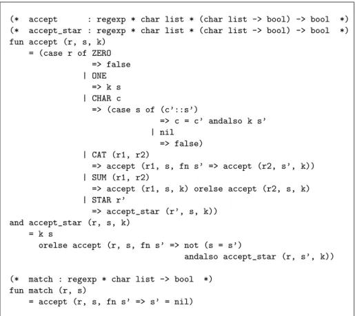
Figure 1: Higher-order, continuation-based matcher for regular expressions
The concatenation of languages is defined as L1L2={x@y|x∈L1∧y∈L2},
where we use the append function (noted@as in ML) to concatenate strings.
5.2 The two matchers
Our reference matcher for regular expressions is higher-order (Figure 1). We then present its defunctionalized counterpart (Figure 2).
5.2.1 The higher-order matcher
Figure 1 displays our reference matcher, which is compositional and continuation-based. Compositional: all recursive calls toacceptoperate on a proper subpart of the regular-expression under consideration. And continuation-based: the control flow of the matcher is driven by continuations.
The main function is match. It is given a regular expression and a list of
characters, and callsacceptwith the regular expression, the list, and an initial
Theacceptfunction recursively descends its input regular expression, thread-ing the list of characters.
Theaccept starfunction is a lambda-lifted version of a recursive continua-tion defined locally in theSTARbranch. (The situation is exactly the same as in a compositional interpreter for an imperative language with while loops, where one writes an auxiliary recursive function to interpret loops.) This recursive continuation checks that matching has progressed in the string.
Recently, Harper has published a similar matcher to illustrate “proof-directed debugging” [25]. Playfully, he considered a non-compositional matcher that does not check progress when matching a Kleene star. His article shows (1) how one stumbles on the non-compositional part when attempting a proof by structural induction; and (2) how one realizes that the matcher diverges for pathologi-cal regular expressions such as STAR ONE. Harper then (1) makes his matcher compositional and (2) normalizes regular expressions to exclude pathological regular expressions. Instead, we start from a compositional matcher and we include a progress test inaccept star, which lets us handle pathological regular expressions.
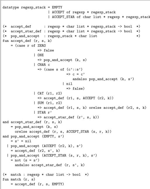
5.2.2 The first-order matcher
Defunctionalizing the matcher of Figure 1 yields a data type representing the continuations and its associated apply function.
The data type represents a stack of regular expressions (possibly with a side condition for the test in Kleene stars). The apply function merely pops the top element off this stack and tries to match it against the rest of the string. We thus name the data type “regexp stack” and the apply function “pop and accept”. We also give a meaningful name to the datatype constructors. Figure 2 displays the result.
5.3 The two correctness proofs
We give a correctness proof of both the higher-order version and the first-order version, and we investigate whether each proof can be converted to a proof for the other version.
The correctness criterion we choose is simply that for all regular expressions
rand stringss(represented by a list of characters),
evaluatingmatch (r, s)terminates, and
match (r, s) true ⇔ s∈ L(r)
When writing match (r, s) true, we mean that evaluating match (r, s)
terminates and yields the result true. We also reason about ML programs equationally, writing e ≡ e0 if e and e0 are defined to be equal, e.g., by a function definition. Ife≡e0 theneande0 evaluate to the same value, if any, so
e v⇔e0 v. We writee=e0 on ML expressions only if they represent the
datatype regexp_stack = EMPTY
| ACCEPT of regexp * regexp_stack
| ACCEPT_STAR of char list * regexp * regexp_stack (* accept_def : regexp * char list * regexp_stack -> bool *) (* accept_star_def : regexp * char list * regexp_stack -> bool *) (* pop_and_accept : regexp_stack * char list *) fun accept_def (r, s, k)
= (case r of ZERO => false | ONE
=> pop_and_accept (k, s) | CHAR c
=> (case s of (c’::s’) => c = c’
andalso pop_and_accept (k, s’) | nil
=> false) | CAT (r1, r2)
=> accept_def (r1, s, ACCEPT (r2, k)) | SUM (r1, r2)
=> accept_def (r1, s, k) orelse accept_def (r2, s, k) | STAR r’
=> accept_star_def (r’, s, k)) and accept_star_def (r, s, k)
= pop_and_accept (k, s)
orelse accept_def (r, s, ACCEPT_STAR (s, r, k)) and pop_and_accept (EMPTY, s’)
= s’ = nil
| pop_and_accept (ACCEPT (r2, k), s’) = accept_def (r2, s’, k)
| pop_and_accept (ACCEPT_STAR (s, r, k), s’) = not (s = s’)
andalso accept_star_def (r, s’, k) (* match : regexp * char list -> bool *) fun match (r, s)
= accept_def (r, s, EMPTY)
5.3.1 Correctness proof of the higher-order matcher
Since match (r, s) ≡ accept (r, s, fn s’ => s’ = nil), by definition, it is
sufficient to prove that forsandras above, and for any function from lists of
characters to booleans terminating on all suffixes ofs, denoted byk,
evaluatingaccept (r, s, k)terminates, and
accept (r, s, k) true ⇔ s∈ L(r)L(k)
where we define the language of a “string-acceptor”kas the set{s|k s true}. The proof is by structural induction on the regular expression. In the case wherer=STAR r’, a subproof shows that the following holds for any string.
evaluatingaccept star (r’, s, k)terminates, and
accept star (r’, s, k) true ⇔ s∈ L(r’)∗L(k)
The subproof is by well-founded induction on the structure of the string (suffixes are smaller) for the “⇐” direction, and by mathematical induction on the nat-ural numbernsuch thats∈ L(r’)nL(k) for the “⇒” direction. Both subproofs use the outer induction hypothesis foraccept (r’, s, k). (See Appendix A.)
We can transfer this proof to the defunctionalized version. Sincek s trans-lates to pop and accept (k, s), we define L(k) to read {s | pop and accept (k, s) true}. The proof then goes through in exactly the same format.
5.3.2 Correctness proof of the first-order matcher
Alternatively, if we were to prove the correctness of the first-order matcher di-rectly, we would be less inclined to recognize the stackkas representing a func-tion. Instead, we could easily end up proving the following three propositions by mutual induction.
P1(r,s,k) def= accept (r, s, k) true ⇔ s∈ L(r)L(k)
P2(k,s) def= pop and accept (k, s) true ⇔ s∈ L(k)
P3(r,s,k) def= accept star (r, s, k) true ⇔ s∈ L(r)∗L(k)
where we define the language of a stack of regular expressions as follows.
L(EMPTY) = {nil}
L(ACCEPT (r, k)) = L(r)L(k)
L(ACCEPT STAR (s, r, k)) = (L(r)∗L(k))\ {s}
For brevity we ignore the termination part of the proof and assume that all the functions are total. We prove, by well-founded induction on the propositions themselves, thatP1,P2, andP3hold for any choices ofs,r, andk. The ordering
is an intricate mapping intoω×ω, ordered lexicographically so that the proof of a proposition only depends on “smaller” propositions. (See Appendix B.)
This proof is more convoluted than the higher-order one for two reasons: 1. it separates the language of the continuation from the function that matches
it, so one has to check whether the function really matches the correct lan-guage; and
2. it combines the two nested inductions of the higher-order proof into one well-founded induction.
Still this proof reveals a property of the continuations in the higher-order version, namely that there are at most three different kinds of continuations in use, something that cannot be seen from the type of the continuation—a full function space.
We could thus define a subset of this function space inductively, so that it only contains the functions that can be generated by the three abstractions. The first-order proof could then be extended to the higher-order program by assuming everywhere that the continuation k lies in this subset and showing that newly generated continuations do too. In effect, the set of continuations is partitioned into disjoint subsets, just as the first-order datatype represents a sum, and then we can prove something about elements in each part.
5.4 Comparison between the two correctness proofs
The proof of correctness of the first-order matcher directly uses the fact that the inductively defined data type representing continuations is a sum. Given a value of this type, we can reason by inversion and do a proof by cases. We show that a proposition holds for each of the three possible summands, and we conclude that the proposition must hold for any value of that type. This is reminiscent of defunctionalization, where in an entire program, the functions occupying a function space are exactly those originating from the function abstractions in the program, which can be represented by a finite sum.
We can translate the proof of the first-order matcher directly into a proof of the higher-order matcher. The resulting proof uses global reasoning, namely that all the used functions arise from only finitely many function abstractions,3
and furthermore that these function abstractions inductively define a subset of the function space. We change the induction hypothesis to assume that the functions are taken from that subset. When instantiating a function abstrac-tion, we must show that the result belongs to the subset—which follows from the assumptions on the free variables—allowing us to use the induction hypothesis on this new function. When using a function, we can then reason by inversion and do a proof by cases to show a property of this function. Each case corre-sponds to an abstraction that can have created this function. We show that a proposition holds for each of the three possible function abstractions, and we conclude that the proposition must hold for the function.
The proof of correctness of the higher-order matcher uses local reasoning instead. We do not assume that the functions lie in the exact subset of the
function space that is generated by the function abstractions. Instead, we as-sume the weaker property that given a string, the function terminates on all suffixes of that string. This assumption is sufficient to complete the proof.
We can translate the proof of the higher-order matcher directly into a proof of the first-order matcher by replacing function abstractions with datatype con-structors and applications with calls to the apply function. The resulting proof uses local reasoning, namely that all the defined functions satisfy a property. The property that the functionkterminates on all suffixes of the current string is translated to the property that pop and accept (k, s’)terminates if s’ is a suffix of the current string. This assumption is then propagated to the calls to
pop and accept.
Therefore, the two proofs differ where the inductive reasoning occurs:
• in the first-order case, the inductive reasoning about a data-type value is carried out at the use point; in contrast, no reasoning takes place where the data-type value is defined; and
• in the higher-order case, the inductive reasoning about a function value is carried out at the definition point; in contrast, no reasoning takes place where the function value is used.
This difference is emphasized by the translations between the proofs. It orig-inates from the different handlings of recursion in the two matchers. In the first-order case, recursion is handled in the case dispatch where the values are used. In the higher-order case, recursion is handled in a function abstraction, which is only available to reason upon where the function is defined.
5.5 Summary and conclusion
We have considered a matcher for regular expressions, both in higher-order form and in first-order form, and we have compared them and their correctness proof. The difference between the function-based and the datatype-based rep-resentation of continuations is reminiscent of the concept of ‘junk’ in algebraic semantics [22]. One representation is a full function space where many elements do not correspond to an actual continuation, and the other representation only contains elements corresponding to actual continuations. This difference finds an echo in the correctness proofs of the two matchers, as analyzed in Section 5.4. More generally, this section also illustrates that defunctionalizing a func-tional interpreter for a backtracking language that uses success continuations yields a recursive interpreter with one stack [13, 31, 41]. Similarly, defunction-alizing a functional interpreter that uses success and failure continuations yields an iterative interpreter with two stacks [13, 34].