Application of an Ant Colony Optimization
Algorithm for Optimal Operation of
Reservoirs: A Comparative Study
of Three Proposed Formulations
R. Moeini
1and M.H. Afshar
1;Abstract. This paper presents an application of the Max-Min Ant System for optimal operation of reservoirs using three dierent formulations. Ant colony optimization algorithms are a meta-heuristic approach initially inspired by the observation that ants can nd the shortest path between food sources and their nest. The basic algorithm of Ant Colony Optimization is the Ant System. Many other algorithms, such as the Max-Min Ant System, have been introduced to improve the performance of the Ant System. The rst step for solving problems using ant algorithms is to dene the graph of the problem under consideration. The problem graph is related to the decision variables of problems. In this paper, the problem of optimal operation of reservoirs is formulated using two dierent sets of decision variable, i.e. storage volumes and releases. It is also shown that the problem can be formulated in two dierent graph forms when the reservoir storages are taken as the decision variables, while only one graph representation is available when the releases are taken as the decision variables. The advantages and disadvantages of these formulation are discussed when an ant algorithm, such as the Max-Min Ant System, is attempted to solve the underlying problem. The proposed formulations are then used to solve the problem of water supply and the hydropower operation of the \Dez" reservoir. The results are then compared with each other and those of other methods such as the Ant Colony System, Genetic Algorithms, Honey Bee Mating Optimization and the results obtained by Lingo software. The results indicate the ability of the proposed formulation and, in particular, the third formulation to optimally solve reservoir operation problems. Keywords: Ant colony optimization; Max-Min Ant System; Graph; Optimal operation of reservoir; Hydropower reservoir.
INTRODUCTION
Many optimization problems of practical, as well as theoretical, importance consist of the search for the \best" conguration of a set of variables to achieve some goals. They seem to be divided naturally into two categories: Those in which the solutions are encoded with real-valued variables and those where solutions are encoded with discrete variables. Among the latter, there is a class of problem called Combinatorial Opti-mization (CO) problems. According to Papadimitriou and Steiglitz [1], in CO problems one is looking for an object from a nite set. Examples of CO problems are
1. Department of Civil Engineering, Iran University of Science and Technology, Tehran, P.O. Box 16765-163, Iran. *. Corresponding author. E-mail: [email protected] Received 17 October 2007; received in revised form 18 September 2008; accepted 8 November 2008
the Traveling Salesman Problem (TSP), the Quadratic Assignment Problem (QAP) and Time Tabling and Scheduling Problems. Due to the practical importance of CO problems, many algorithms have been developed to tackle them [2].
In the last 20 years, a new kind of approximate optimization method has emerged, which basically tries to combine basic heuristic methods with higher level frameworks aimed at eciently and eectively exploring a search space. These methods are nowadays commonly called metaheuristics. Before this term was widely adopted, metaheuristics were often called modern heuristics. This class of algorithm includes, but is not restricted to, Ant Colony Optimization (ACO) and Evolutionary Computation (EC), including Genetic Algorithms (GA), Iterated Local Search (ILS), Simulated Annealing (SA), and Tabu Search (TS). Up to now there has not been any commonly accepted
denition for the term meta-heuristics. It is just in the last few years that some researchers in the eld have tried to propose a denition [2].
Within the last decade, many researchers have shifted the focus of optimization problems from tra-ditional optimization techniques, based on linear and non-linear programming, to the implementation of Evolutionary Algorithms (EAs), Genetic Algorithms (GAs), Simulated Annealing (SA) and Ant Colony Optimization (ACO) algorithms.
ACO is a metaheuristic approach proposed by Cloroni et al. [3] and Dorigo et al. [4]. The basic algorithm of ant colony optimization is the Ant System (AS). Many other algorithms have been introduced to improve the performance of the Ant System such as Ant Colony System (ACS), Elitist Ant System (ASelite),
Elitist-Rank Ant System (ASrank) and Max-Min Ant
System (MMAS) [5]. Advancements have been made on the initial and most simple formulation of ACO, the Ant System (AS), to improve the operation of the decision policy and the manner in which the policy incorporates new information to help explore the search space. These developments have primarily been aimed at managing the trade-o between the two conicting search attributes of exploration and exploitation.
In this paper, MMAS is applied to the problem of reservoir operation. Three dierent formulations are presented to cast the underlying problem into a form suitable for the application of MMAS. Two of these formulations use storage volumes as the decision variables, while the other formulation considers the releases as the decision variable of the problem. With the releases taken as the decision variable, referred to as rst formulation, each period of the operation is considered as the decision point of the problem. Discretizing the range of possible values of release at each period, the options available at each decision point are then represented by the set of discretized values of the releases. When storage volumes are taken as the decision variables, two dierent formulations are possi-ble. In the rst representation, referred to as the second formulation, the beginning and end of each period are taken as the decision points of the problem. Having discretized the range of possible values of storage volumes at each decision point, the options available are then represented by the set of discretized values of the storage volumes at each decision point. In this representation, it is not possible to associate a cost with the options available at each decision point due to the fact that the cost function of the problems considered is a function of release. In the second representation of the reservoir operation problem, with storage volumes taken as decision variables and referred to as the third formulation, the beginning and end of each period are again taken as the decision points of the problem, as in the second formulation. Having discretized the
range of allowable storage volume at all decision points, available options at each decision point are represented now by the arcs joining each and every one of the dis-cretization points to all disdis-cretization points of the next decision point. This formulation oers the advantage of dening a heuristic value for all the dierent operation problems, since each arc uniquely denes the operation policy of the corresponding period. The formulations so constructed are applied to solve the water supply and hydropower operation problems of the \Dez" reservoir and the results are presented. The results indicate the MMAS is a suitable method for the solution of reservoir operation problems compared to other ant algorithms. The results also indicate that the third formulation is superior to other formulations when solving larger scale water supply operation problems.
In what follows, the Ant Colony Optimization Algorithm (ACOA) is rst described. The Max-Min Ant System is then presented. The proposed formulations of the reservoir operation problem are presented in the next section. And, nally, the \Dez" reservoir operation problem is solved using MMAS and proposed formulations and the results are presented and compared to the existing results.
ANT COLONY OPTIMIZATION ALGORITHM (ACOA)
Ant algorithms were initially inspired by the observa-tion that ants can nd the shortest path between food sources and their nest, even thought they are almost blind [4]. Individual ants choose their path from the nest to the food source in an essentially random fashion. While walking from the food source to the nest and vice versa, the ants deposit on the ground a substance called pheromone forming, in this way, a pheromone trail. Ants can smell pheromone and they tend to choose paths marked by strong pheromone concentrations when choosing their way [6]. The pheromone trail acts as a form of indirect communication called stigmergy, helping the ants to nd their way back to the food source or the nest. Also, it can be used by other ants to nd the location of the food source [7,8].
Based upon this ant behavior, Cloroni et al. [3] and Dorigo et al. [9] developed ACO method. In the Ant Colony Optimization meta-heuristic, a colony of articial ants cooperates in nding good solutions to dicult discrete optimization problems [10]. The original and simplest ACO algorithms used to solve many dicult combinatorial optimization problems are TSP [6], graph coloring [11] and network routing [12].
The searching behavior of ant algorithms can be characterized by two main features, exploration and exploitation. Exploration is the ability of the algorithm to broadly search through the solution space, whereas exploitation is the ability of the algorithm to search
thoroughly in the local neighborhood, where good solu-tions have previously been found. Higher exploitation is reected in rapid convergence of the algorithm to a suboptimal solution, whereas higher exploration results in better solutions at higher computational cost due to the slow convergence of the method. Dierent methods have been developed for a proper trade-o between exploration and exploitation in ant algorithms.
Application of ant algorithms to an arbitrary combinatorial optimization problem requires that the problem be projected on a graph [9]. Consider a graph, G = (D; L; C) in which D = fd1; d2; ; dng is the
set of decision points at which some decisions are to be made, L = flijg is the set of options (arcs) j,
(j = 1; 2; ; J), at each of the decision points i, (i = 1; 2; ; n), and nally C = fcijg is the set of costs
associated with options L = flijg. The components of
sets D and L may be constrained if required. A feasible path on the graph is called a solution (') and the minimum cost path on the graph is called the optimal solution ('). The cost of the solution is denoted by
f(') and the cost of the optimal solution by f(').
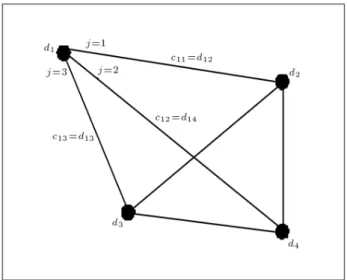
ACOA was used rst for the Traveling Salesman Problem (TSP). In TSP, each ant starts from an arbitrary city and, while passing all other cities, goes back to the starting city. The object of this problem is to nd the shortest path covering all cities only once. The graph of this problem is presented in Figure 1. Each city is considered as a decision point, therefore, the number of decision points is equal to the number of cities. Each option (arcs) denes the path taken from one city to another. In TSP, each city (decision point) is connected to all other cities (decision points) and, hence, the use of a fully connected graph. This means that in TSP each ant is faced with the total number of options nearly equal to the number of cities. When an option (arc) is chosen by an ant, the next city (decision
Figure 1. Basic graph for TSP.
point) to move to is known. The cost of each option is equal to the distance between two cities.
The basic steps of the ant algorithm may be dened as follows [10]:
1. m ants are randomly placed on n decision points, and the amounts of pheromone trail on all arcs are initialized to some proper value at the start of the computation.
2. A transition rule is used at each decision point, i, to decide which option is to be selected. The ants move to the next decision point and the solutions are incrementally created by ants as they move from one point to the next. This procedure is repeated until all decision points of the problem are covered. The transition rule used in the original Ant System is dened as follows [10]:
Pij(k; t) = [ij(t)] [
ij] J
P
j=1[ij(t)] [ij]
; (1)
where:
Pij(k; t) the probability that ant k selects option
Lij(t) for the ith decision point at
iteration t;
ij(t) the concentration of pheromone on
option (arc) Lij(t) at iteration t;
ij the heuristic value representing the cost
of choosing option j at point i;
the parameter that control the relative weight of the pheromone trail;
the parameter that controls the relative weight of the heuristic value.
The heuristic value (ij) is analogous to
pro-viding the ants with sight and is sometimes called visibility. This value is calculated once at the start of the algorithm and is not changed during the computation.
3. Costs, f('), of the trail solutions generated are calculated. The generation of a complete trail solution and calculation of the corresponding cost is called the cycle (k).
4. The pheromone is updated after steps 2 and 3 are repeated for all ants and, therefore, the generation of m trail solutions and calculation of their corre-sponding costs are referred to as iteration (t). The general form of the pheromone updating rule is as follows:
where:
ij(t+1) the amount of pheromone trail on option
j at the ith decision point, which is option Lij at iteration t + 1;
ij(t) the concentration of pheromone on
option Lij at iteration t;
the coecient representing the pheromone evaporation (0 1); ij the change in pheromone concentration
associated with option Lij.
Dierent methods have been developed for calculating the change of pheromone, ij, one of which is the
Max-Min Ant System [13]. MAX-MIN ANT SYSTEM
Premature convergence to suboptimal solutions is an issue that can be experienced by all ant algorithms. To overcome the problem of premature convergence, whilst still allowing for exploitation, Stutzle and Hoss [14,15] developed the Max-Min Ant System (MMAS). The basis of MMAS is the provision of dynamically evolving bounds on the pheromone trail intensities, such that the pheromone intensity on all paths is always within a specied lower bound, min(t), of a theoretically
asymp-totic upper limit, min(t), that is min(t) ij(t)
max(t) for all edges (i; j). As a result of the lower
bound stopping the pheromone trails from decaying to zero, all paths always have a nontrivial probability of being selected and, thus, a wider exploration of the search space is encouraged. The upper pheromone bound at iteration t is given by:
max(t) = 1 1 f(sgb(t)); (3)
where:
max(t) upper bound of pheromone trail at
iteration t;
the coecient representing pheromone evaporation (0 1);
rewarding factor (usually = 1); f(sgb(t)) cost of the best global solution at
iteration t.
This expression is equivalent to the asymptotic limit of an edge receiving pheromone additions of
f(sgb(t))and decaying by a factor of (1 ) at the end of each iteration. The lower bound at iteration t is given by:
min(t) =max(t) 1
n p
Pbest
(NOavg 1)pnPbest ; (4)
where Pbest(0Pbest1) is a specied probability that
the current global-best path (sgb(t)) will be selected,
given that no global best edge has a pheromone level of min(t) and all global-best edges have a pheromone
level of max(t); and NOavg is the average number of
edges across all decision points.
It should be noted that a lower value of Pbest indicates tighter bounds. Theoretical
justica-tion of min(t) and max(t) is given in Stutzle and
Hoos [16].
As the bounds serve to encourage exploration, provision for exploitation is made in MMAS by addi-tion of pheromone to only the iteraaddi-tion-best ant path (sl(t)) at the end of an iteration and, to further exploit,
the global-best solution (sgb(t)) is updated every T gb
iterations. The MMAS updating scheme is given by: ij(t + 1) = ij(t) + ijib(t) + ijgb(t)IN
t Tgb
; (5) where N is the set of natural numbers (note, t
Tgb is an element of N in every Tgbiteration), and ijib(t) is the
pheromone addition given by iteration-best ant (sl(t)),
which is dened as below: ib
ij(t) =f(s
l(t))Isl(t)f(i; j)g; (6)
where:
the coecient (usually = 1);
f(sl(t)) cost of best global solution at iteration t;
Isl(t)=1 if arc (i; j) is chosen by best ant (ib); Isl(t)=0 otherwise.
Application of MMAS to some benchmark combi-natorial optimization examples such as the Traveling Salesman Problem (TSP), has shown that it over-comes the stagnation problem and, hence, improves the performance of the ant algorithms for the range of problems considered.
FORMULATION OF THE RESERVOIR OPERATION PROBLEMS
A variety of reservoir operation problems have been devised and solved with dierent methods. Three major modeling approaches that have been widely used for optimization of reservoir operation problems are: Linear Programming (LP), Non-Linear Program-ming (NLP) and Dynamic ProgramProgram-ming (DP). Ap-plication of DP techniques to water resource systems has been reviewed by Yakowitz [17]. Marino and Loaiciga [18] and Becker and Yeh [19] solved the optimal operation of reservoirs with DPs. Recently, Mousavi and Karamouz [20] improved the DP mod-els by diagnosing infeasible storage combinations and using the results for solving multi-reservoir operation problems. However, the main shortcoming of DP
is the exponential increase in computational burden and memory requirements, known as the curse of dimensionality, as the number of state variables in-crease. Thus, the applicability of DP is limited to systems with very few reservoirs. To partially overcome the dimensionality problem in dynamic programming, evolutionary algorithms have been used. There have been several applications of GAs to multi-reservoir operation problems [21-23]. Esat and Hall [21] clearly demonstrated the advantages of GAs over standard dynamic programming techniques in terms of compu-tational requirements. Wardlaw and Sharif [24] applied GAs to a four-reservoir system operation problem concluding that GA's with real value coding perform signicantly faster than those employing binary coding. They extended the formulation to a more complex ten-reservoir problem. Being at its early stages of development, a Honey-Bee Mating Optimization (HBMO) meta-heuristic algorithm was applied to a single reservoir operation problem [25]. Recently, Jalali et al. used a multi-colony ant colony opti-mization algorithm to solve a ten-reservoir operation problem [26].
With a view to handle the scale aspect of the reservoir operation problem using heuristic search methods, such as ACOA uses here, only reservoir oper-ations for the water supply and reservoir operoper-ations for the hydropower generation of a single reservoir with a known storage volume at the start of the operation are considered in this paper. The extension of the methods to multi-reservoir problems will pose no problem once the basics of the methods are understood.
Reservoir Operation for Water Supply
Optimal operation of a single reservoir for water supply may be stated mathematically as follows:
Minimize F =
NTP
t=1[D(t) r(t)] 2
Dmax ; (7)
subject to continuity equations at each period:
s(t + 1) = s(t) + I(t) r(t) l(t); (8)
and minimum and maximum allowable values for the release and storage volumes at each period:
smin s(t) smax; (9)
rmin r(t) rmax; (10)
where:
NT total number of periods; D(t) water demand in time period t;
r(t) water release from the reservoir in time period t;
Dmax maximum water demand (constant);
s(t) reservoir storage at the beginning of period t;
I(t) water inow to the reservoir in period t; r(t) water release from the reservoir in period t; l(t) evaporation loss in period t;
smin minimum water storage of the reservoir;
smax maximum water storage of the reservoir;
rmin minimum water release from the reservoir;
rmax maximum water release from the reservoir.
Optimal Reservoir Operation for Hydropower Generation
The problem of optimal reservoir operation for hy-dropower generation is often stated mathematically as follows:
Minimize F =
NT
X
t=1
1 powerp(t)
; (11)
where:
NT total number of time periods;
p(t) power generated by the hydro-electric plant in period t;
Power total capacity of hydro-electric plant (MW). The power generated by the plant is dened as:
p(t) = min
g R(t) PF
ht
1000
; power
; (12) with:
ht=
H
t+ Ht+1
2
T W L; (13)
where:
p(t) power generated in period t (MW); g gravity acceleration (m2/s);
eciency of hydro-electric plant; PF plant factor;
ht eective head of hydro-electric plant in
period t;
Ht elevation of water in the reservoir in period
t;
TWL tail water elevation of hydro-electric plant (constant);
R(t) turbine release (release rate from reservoir, (m3/s)).
Subject to the continuity equation of the reservoir at each period:
s(t + 1) = s(t) + I(t) r(t) l(t); (14) and minimum and maximum allowable values for the release and storage volumes at each period and mini-mum power yield and turbine release at each period:
smin s(t) smax; (15)
rmin r(t) rmax; (16)
p(t) pmin; (17)
R(t) Rmin: (18)
s(t) reservoir storage at the beginning of period t;
I(t) water inow to the reservoir in period t; r(t) water release from the reservoir in period t; l(t) evaporation loss in period t;
smin minimum water storage of reservoir;
smax maximum water storage of reservoir;
rmin minimum water release from reservoir;
rmax maximum water release from reservoir;
pmin minimum power yield;
Rmin minimum turbine release.
R(t) = co(t) r(t); (19)
where co(t) = time coecient for period t and other parameters are dened as before.
The water elevation can be obtained from the volume-elevation curve dened as follows:
Hi= a + b si+ c s2i + d s3i; (20)
where a; b; c; d = constant coecients obtained by tting the above equation to the data available. Proposed Formulations
Formulation of the optimal operation of reservoirs as an optimization problem requires the selection of decision variables. Basically, two dierent sets of decision variable can be sought in reservoir operation problems, namely storage volumes (s) or releases (r) at each period. Furthermore, application of ant algorithms, such as MMAS, requires that the problem under con-sideration be presented in terms of a graph by dening decision points, options available at each decision point and costs associated with each of these options. The problem graph is very much dependant on the decision variables selected for the problem.
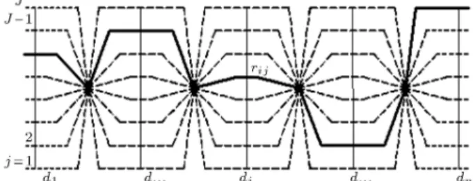
With the releases taken as the decision variables, the problem graph can be dened as illustrated in
Figure 2. Basic graph when release is the decision variable (rst formulation).
Figure 2. In this representation, referred to as rst formulation, each period of the operation is considered as the decision point of the problem. Discretizing the range of possible values of release in each period, the options available at each decision point are then represented by the set of discretized values of the releases. It is to be noted that the options are, in fact, represented by the set of discretization points rather than arcs in its real sense. When the initial reservoir storage is unknown, this parameter is also taken as a decision variable leading to a problem with total of NT + 1 decision variables. For the rst problem, a cost can be associated to each option j at decision point i, which is dened as the squared deviation of the release from the required demand at that period. The corresponding heuristic value can, therefore, be dened as:
ij =(D(t) r1
ij)2; (21)
where:
ij heuristic value at arc (i; j);
D(t) water demand at period t (decision point i); rij jth discretized release from reservoir at
period (decision point) i.
Denition of a cost for each option in a hydropower reservoir operation problem, however, is not possible in this formulation, since it requires the value of the eective head, which is not known. Note that the eective head is a function of the storage volumes at the beginning and end of the period.
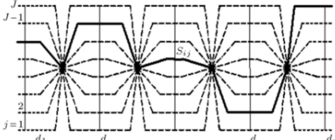
The situation is somehow dierent when storage volumes are taken as the decision variables. In this case, the problem can be represented by two dierent graphs. In the rst representation, referred to as second formulation, the beginning and end of each period are taken as the decision points of the problem, as illustrated in Figure 3. Discretizing the range of possible values of storage volume at each decision point, the options available are then represented by the set of discretized values of the storage volumes at that decision point. In this formulation, it is not possible to associate a cost to the options available
Figure 3. Basic graph when storage is decision variable (second formulation).
at each decision point, due to the fact that the cost function of both water supply and hydropower reservoir operation problems are functions of release. It is clear that the amount of release can only be known when the storage volumes are known at both the beginning and end of the period. Two notes have to be made regarding the characteristics of this formulation. First, the options available at dierent decision points are independent from each other and, therefore, the decisions made at for example two consecutive decision points can be made arbitrarily, as shown in Figure 3. Second, available options at each decision point are in fact some points chosen on the range of possible values of the decision variable associated with that decision point. There is no arc in the sense that exists in TSP problem in this formulation of the reservoir operation problem. The pheromones are, therefore, associated to this point rather than the arcs in its true meanings. This is somehow related to the fact that no heuristic infor-mation can be dened for options in this representa-tion.
In the second representation of the reservoir operation problem with the storage volumes taken as decision variables, referred to as the third formulation, the beginning and the end of each period are taken as the decision points of the problem, as in the second formulation. Having discretized the range of allowable storage volumes at all decision points, one can represent available options at each decision point as shown in Figure 4 by the arcs joining each and every one of the discretization points to all discretization points of the next decision point. This formulation diers from the second formulation in two ways. First, the options available to the ants at each decision point are not independent from decisions made at previous decision points. To be specic, the options (arcs) available at decision point i are very much related to the decisions made at previous decision points and, in particular, at decision point i 1. This is a direct result of the physical requirement that a storage volume at the end of each period should be the same as a storage volume at the beginning of the next period. This property is very useful, as it takes into account the serial feature of
Figure 4. Basic graph when storage is decision variable (third formulation).
the reservoir operation problem. The associated graph is, in fact, very similar to the graph constructed in the dynamic programming method for a total enumeration. The second dierence, very much related to the rst, is that the options are, in fact, real arcs joining the value of the storage volumes at the beginning and the end of each period. This is very signicant, as it is now possible to dene heuristic information for all the options (arcs) at any of the decision points, since a release value can be computed for each and every arc using the storage volumes at the beginning and end of the arc and the continuity equation. It is interesting to note that useful heuristic information can be easily computed for both of the reservoir operation problems considered here. The heuristic value is calculated by Equation 21 for water supply reservoir operations and Equation 22 for hydropower operation problems.
ij = 1 powerpij ; (22)
where:
ij the heuristic value at arc (i; j);
Power total capacity of hydro-electric plant; pij power generated by the power plant, which
can be calculated by Equation 15 using the known storage volumes and release during the period.
To discourage the ants from making decisions (i.e. select releases or storages) that constitute an infeasible solution, a higher cost is associated to the solutions that violate constraints of the problem. This is achieved via the use of a penalty method, in which the total cost of the problems is considered as the sum of the problem costs and a penalty cost as follows:
Fp= F + p NT
X
t=1
CSVt; (23)
F original objective function dened by Equaitons 7 and 11 for the water supply and hydropower cases, respectively; Fp penalized objective function;
CSVt a measure of constraint violation at period
t;
p represents the penalty parameter.
TEST EXAMPLES
In this section, the water supply and hydropower operation of the \Dez" reservoir in southern Iran are considered as test examples to test the versatility and eciency of the proposed formulations. The active storage volume of the \Dez" reservoir is equal to 2510 MCM, and its average annual inow is equal to 5303 MCM over 5 years and 5900 MCM over 40 years. These problems are solved here for optimal monthly operation over 5 and 20 years, i.e. 60 and 240 monthly periods, respectively. The initial storage of the reservoir is taken equal to 1430 MCM. The maximum and minimum allowable storage volumes are considered equal to 3340 MCM and 830 MCM, respectively, while maximum and minimum monthly water releases are taken to be 1000 MCM and zero, respectively. Evaporation losses in each period, minimum power yield and turbine releases are considered to be equal to zero.
For hydropower reservoir operation problem, a polynomial is tted to the volume-elevation data, dened as follows:
Hi= 249:83364 + 0:0587205 si 1:37 10 5
s2
i + 1:526 10 9 s3i: (24)
The \Dez \reservoir hydro-electric plant consists of eight units. Each unit has a capacity of 80.8 MW and is supposed to work 10 hours per day leading to a plant factor of 0.417. The total capacity of the hydro-electric plant of the \Dez" reservoir is equal 650 MW and its eciency equals 90 percent ( = 0:9). The downstream elevation of the hydro-electric plant from the sea surface equals 172 meters (T W L = 172 meter above sea level).
RESULTS AND DISCUSSIONS
In this section, the results obtained for optimal op-eration of the \Dez" reservoir, using the proposed
formulations, are presented and compared to results obtained by other methods. All the results presented hereafter are based on an iteration best pheromone updating mechanism, neglecting the role of a global-best solution in Equation 6, and uniform discretization of the allowable range of decision variables into 18 intervals for rst formulation and 36 intervals for the second and third formulations.
First, consider the solution of the water supply and hydropower operation using the rst formulation, in which the releases are taken as the decision vari-ables of the problem. The graph of the problem is already shown in Figure 2. A set of preliminary runs are conducted to nd the proper values of MMAS parameters as shown in Table 1. Table 2 shows the results of 10 runs carried out for the problems of water supply and hydropower operation of the \Dez" reservoir using the parameters of Table 1 over 60 and 240 monthly periods. These results are obtained within 2000 iterations, amounting to 400,000 function evaluations for each run using a colony size of 200.
As seen from Table 2, optimal solutions obtained using the rst formulation for water supply operations over 60 and 240 months have costs of 0.785 and 10.314 units, respectively. Optimal solutions obtained using the rst formulation for hydropower operations over 60 and 240 months have costs of 7.913 and 35.3 units, respectively. These can be compared with the costs of 0.7316 and 4.7684 obtained with Lingo software (version 9) for water supply over 60 and 240 months, respectively, and 7.372 and 20.622 obtained with Lingo software for hydropower operation over 60 and 240 months, respectively. It is clear that MMAS is able to produce a near-optimal solution for both cases of water supply and hydropower operation problem. These problems were also solved by Jalali et al. [26] using standard and improved Ant Colony System (ASC). Standard ACS required 400,000 function evaluation to get to a solution of 0.926 for water supply operation over 60 monthly periods. The improved version of ACS, on the other hand, was able to obtain the solution of 0.804 for water supply reservoir over 60 monthly
pe-Table 1. Values of MMAS parameters used in the rst formulation.
NO. Ant pbest
200 1 0.1 0.9 0.15
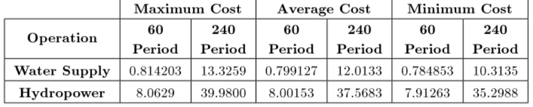
Table 2. Maximum, minimum and average solution costs over 10 runs (rst formulation). Maximum Cost Average Cost Minimum Cost Operation 60
Period
240 Period
60 Period
240 Period
60 Period
240 Period Water Supply 0.814203 13.3259 0.799127 12.0133 0.784853 10.3135 Hydropower 8.0629 39.9800 8.00153 37.5683 7.91263 35.2988
riods with 400,000 function evaluations. The problem of water supply operation of \Dez" reservoir over 60 monthly periods was also solved by Bozorg Haddad et al. [25] using GA and HBMO algorithms to only achieve solutions of 1.1 and 0.82 using 6,000,000 function evaluations, respectively. Also, standard ACS failed to produce a feasible solution for hydropower operation over 60 monthly periods. The improved version of ACS, on the other hand, was able to obtain the solution of 7.504 for hydropower reservoir over 60 monthly periods with 1,000,000 function evaluations. It is clearly seen that for both problems, MMAS was able to obtain better solutions than standard and improved ACS, GA and HBMO algorithms. The CPU time required by MMAS for each run carried out on a 2.4 MHZ Pentium PC, were about 300(320) and 1220(1250) seconds for water supply (hydropower) operation over 60 and 240 monthly periods, respectively. Figures 5 to 8 show the variation of maximum, minimum and average solution costs of water supply and hydropower
Figure 5. Variation of maximum, minimum and average solution costs of water supply operation over 60 periods (rst formulation).
Figure 6. Variation of maximum, minimum and average solution costs of water supply operation over 240 periods (rst formulation).
Figure 7. Variation of maximum, minimum and average solution costs of hydropower operation over 60 periods (rst formulation).
Figure 8. Variation of maximum, minimum and average solution costs of hydropower operation over 240 periods (rst formulation).
operation of \Dez" reservoir over 60 and 240 monthly periods obtained using the rst formulation in which the releases are taken as the decision variables.
Next, these problems are solved using the second formulation in which the storage volumes are taken as the decision variables of the problem. Following a set of preliminary runs, the values of MMAS parameters listed in Table 3 are selected for the main runs. Again to assess the sensitivity of the proposed formulation to initial random colony, the problems are solved with ten dierent initial colonies. Table 4 shows the maximum, minimum and average solution costs of water supply and hydropower operation of \Dez" reservoir over 60 and 240 monthly periods obtained
Table 3. Value of MMAS parameters in the second formulation.
NO. Ant pbest
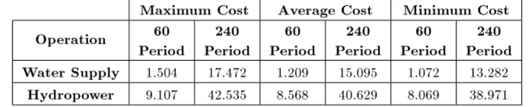
Table 4. Maximum, minimum and average solution costs over 10 runs (second formulation). Maximum Cost Average Cost Minimum Cost Operation 60
Period
240 Period
60 Period
240 Period
60 Period
240 Period Water Supply 1.504 17.472 1.209 15.095 1.072 13.282
Hydropower 9.107 42.535 8.568 40.629 8.069 38.971
using the second formulation in which the storage volumes are taken as the decision variables. It is seen that all the results obtained with this formulation is inferior to those obtained with the rst formulation. This can be attributed to two following dierences. First, the second formulation as explained earlier does not allow for the denition of heuristic information neither in water supply operation nor in hydropower. This of course only explains the superiority of the rst formulation in the case of water supply operation. The second reason for inferior performance of the second formulation can be due to the fact that the original continuous search space is represented by a coarser discrete search space when storage volumes are taken as the decision variables. This can be easily seen by a comparison between allowable range of storage volumes (830-3340) and release volumes (0.0-1000). It should be noted that in this case no heuristic information can be dened for the options available at decision points of the problem and, therefore, the value of = 0:0 is used in the second formulation.
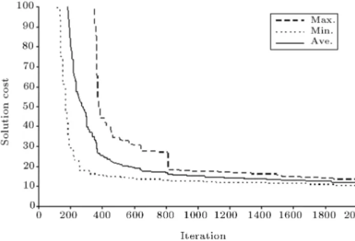
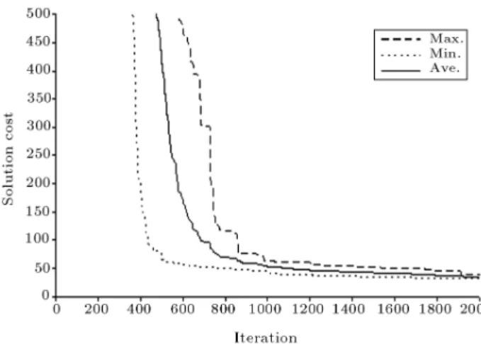
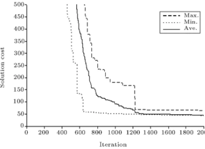
Figures 9 to 12 show the variation of maximum, minimum and average solution costs of the water sup-ply and hydropower operation of the \Dez" reservoir over 60 and 240 monthly periods obtained using the second formulation, in which the storages are taken as the decision variables.
The CPU times required by MMAS for each run carried out on a 2.4 MHZ Pentium PC, are about
Figure 9. Variation of maximum, minimum and average solution costs of water supply operation over 60 periods with iterations (second formulation).
530(340) and 2120(2160) seconds for the water sup-ply (hydropower) operation over 60 and 240 monthly periods, respectively.
The third formulation is also tested on these problems using the MMAS parameters listed in Table 5, which are obtained by some preliminary runs for the best performance of the algorithm. Again, ten runs are carried out to eliminate the eect of an initial colony on the nal solutions obtained. The performance of the third formulation over 10 runs is shown in Table 6 for the two operation problems over 60 and
Figure 10. Variation of maximum, minimum and average solution costs of water supply operation over 240 periods with iterations (second formulation).
Figure 11. Variation of maximum, minimum and average solution costs of hydropower operation over 60 periods with iterations (second formulation).
Figure 12. Variation of maximum, minimum and average solution costs of hydropower operation over 240 periods with iterations (second formulation).
Table 5. Value of MMAS parameters in the third formulation.
NO. Ant pbest
200 1 0.3 0.9 0.15
240 monthly periods. Comparison of these results with those obtained with the second formulation reveals full superiority of the third formulation over the second. Comparison of the results with those obtained by the rst formulation in which the releases are taken as decision variables, listed in Table 2, is noteworthy. In the water supply operation problem, the best solution obtained by the third formulation, 0.830, is slightly inferior to that obtained by the rst formulation, 0.785, over a shorter period of 60 months, while the optimal solution produced by the third formulation over a longer period of 240 months, 7.370, is considerably better than that of the rst formulation, 10.313. This superiority is even more apparent for the worst and average solution costs, showing that the third formu-lation is less sensitive to the initial colony, which is considered to be a useful property for stochastic search methods. The performance of the third formulation for hydropower operation, however, is not as good as the rst formulation, as one might have expected. This can be attributed to the fact that the value of the heuristic information for some arcs, those for which p(t) power, is innity which is replaced by the
maximum heuristic value of all arcs. This will lead to the same heuristic value for some of the arcs leading to poorer results than expected. Figures 13 to 16 show the variation of maximum, minimum and average solution costs for water supply and hydropower operation over 60 and 240 periods considered here.
The CPU time required by MMAS for each run, carried out on a 2.4 MHZ Pentium PC, is about 550(360) and 2200(2240) seconds for the water sup-ply (hydropower) operation over 60 and 240 monthly periods, respectively.
Figure 13. Variation of maximum, minimum and average solution costs of water supply operation over 60 periods with iterations (third formulation).
Figure 14. Variation of maximum, minimum and average solution costs of water supply operation over 240 periods with iterations (third formulation).
Table 6. Maximum, minimum and average solution costs over 10 runs (third formulation). Maximum Cost Average Cost Minimum Cost Operation 60
Period
240 Period
60 Period
240 Period
60 Period
240 Period Water Supply 1.097 8.201 0.922 7.664 0.830 7.370
Figure 15. Variation of maximum, minimum and average solution costs of hydropower operation over 60 periods with iterations (third formulation).
Figure 16. Variation of maximum, minimum and average solution costs of hydropower operation over 240 periods with iterations (third formulation).
CONCLUSION
In this paper, three dierent formulations were used to represent the water supply and hydropower reservoir operation problems in proper form, to be solved with ant colony optimization algorithms. In the rst formu-lation, each period was taken as the decision point of the problem at which the value of the release, as the decision variable, is to be decided. This formulation allowed for denition of the heuristic information only for the case of water supply operation problem. In the second formulation, the beginning and the end of each period were taken as the decision points of the problem and the value of the storage volume was considered as the decision variable. This formulation, however, did not allow for the heuristic information to be dened for options available for none of the problems considered. In the third representation of the reservoir operation problem, with storage volumes taken as decision variables, the beginning and end of each period were taken as the decision points of
the problem. Having discretized the allowable range of storage volumes at all decision points, one could represent available options at each decision point by the arcs joining each and every one of the discretization points to all discretization points of the next decision point. With this representation, it was possible to dene the heuristic information for the options avail-able at any of the decision points, since a release value can be computed for each and every arc using the storage volumes at two ends of the arc and the continuity equation. A recent variant of the ACOA's, namely MMAS, was then used to solve the problem of the water supply and hydropower reservoir operation problems over 5 and 20 years and the results were presented and compared to the available solutions. The results indicated the superiority of the MMAS, in conjunction with the third formulation, over other available methods.
REFERENCES
1. Papadimitriou, C.H. and Steiglitz, K., Combinatorial Optimization-Algorithms and Complexity, Dover Pub-lications Inc., New York (1982).
2. Blum, C. and Roli, A. \Meta-heuristics in combinato-rial optimization: Overview and conceptual compar-ison", ACM Computing Surveys, 36(3), pp. 268-308 (2003).
3. Colorni, A., Dorigo, M. and Maniezzo, V. \Dis-tributed optimization by ant colonies", in Proceedings of ECAL91-European Conference on Articial Life, Elsevier Publishing, pp. 134-142 (1991).
4. Dorigo, M., Maniezzo, V. and Colorni, A. \The ant system: ant autocatalytic optimization process", Technical Report TR 91-016, Politiecnico di Milano (1991)
5. Zecchin, C.A., Maier, H.R., Simpson, A.R., Leonard, M. and Nixon, J.B. \Ant colony optimization applied to water distribution system design: A comparative study of ve algorithms", ASCE, Journal of Water Resources Planning and Management, 133(1), pp. 87-92 (2007)
6. Dorigo, M. and Gambardella, L.M. \Ant colony for the traveling salesman problem", Biosystems, 43, pp. 73-81 (1997).
7. Dorigo, M., Ant Colony Optimization Web Page, http:// iridia.ulb.ac.belmdorigo/ACO/ACO.html. 8. Dorigo, M. and Di Caro, G. \The ant colony
optimiza-tion meta-heuristic", in New Ideas in Optimizaoptimiza-tion, D. Corne, M. Dorigo and F. Glover, Eds., London, UK, McGraw Hill, pp. 11-32 (1999).
9. Dorigo, M., Maniezzo, V. and Colorni, A. \The ant sys-tem: optimization by a colony of cooperating agents, IEEE transaction on systems", Man, Cybernetics-Part B, 26, pp. 29-41 (1996).
10. Dorigo, M., Di Caro, G. and Gambardella, L.M. \Ant algorithms for discrete optimization", Articial Life, 5(2), pp. 137-172 (1999).
11. Costa, D. and Hertz, A. \Ants can color graphs", J. Operate Res. Soc., 48, pp. 295-305 (1997).
12. Di Caro, G. and Dorigo, M. \Two ant colony algo-rithms for best-eort quality of service routing", Un-published at ANTS'98-From Ant Colonies to Articial Ants: First International Workshop on Ant Colony Optimization (1998).
13. Stutzle, T. and Hoss, H. \MAX-MIN ant system and local search for combinatorial optimization prob-lems", in Meta Heuristics: Advances and Trends in Local Search Paradigms for Optimizaiton, S. VOB, S. Martello, I.H. Osman and C. Roucairol, Eds., Kluwer, Boston, pp. 137-154 (1998)
14. Stutzle, T. and Hoos, H. \MAX-MIN ant system", Future Generation Computer Systems, 16(8), pp. 889-914 (2000).
15. Stutzle, T. and Dorigo, M. \A short convergence proof for a class of ACO algorithms", IEEE Transactions on Evolutionary Computation, 6(4), pp. 358-365 (2002). 16. Stutzlt, T. and Hoos, H. \Improvements on the
ant system: Introducing MAX-MIN ant system", in Proceeding of International Conference on Articial Neural Networks and Genetic Algorithms, Springer Verlag, Wien, pp. 245-249 (1997).
17. Yakowitz, S. \Dynamic programming application in water resources", Water Resource Research, 18(4), pp. 673-96 (1982).
18. Marino, M.A. and Loaiciga, H.A. \Dynamic model for multi reservoir operation", Water Resource Res., 21(5), pp. 619-630 (1985).
19. Becker, L. and Yeh, W. \Optimization of real-time operation of a multiple reservoir system", Water Re-source Res., 10(6), pp. 1107-1112 (1974).
20. Mousavi, S.J. and Karamouz, M. \Computational improvement for dynamic programming models by diagnosing infeasible storage combinations", Advances in Water Resources, 26, pp. 851-859 (2003).
21. Esat, V. and Hall, M.J. \Water resource system optimization using genetic algorithms", Hydro Infor-matics'94, Pro., 1st Int. Conf. on Hydro Informatics, Balkerma, Rotterdam, The Netherlands, pp. 225-231 (1994).
22. Fahmy, H.S., King, J.P., Wentzle, M.W. and Seton, J.A. \Economic optimization of river management using genetic algorithms", Int. Summer Meeting, AM. Soc. Agric. Engrs., Paper no. 943034, St. Joseph, Mich. (1994).
23. Oliveira, R. and Loucks, D. \Operation rules for multireservoir systems", Water Resource. Res., 33(4), pp. 839-852 (1997).
24. Wardlaw, R. and Sharif, M. \Evaluation of genetic algorithms for optimal reservoir system operation", Journal of Water Resources Planning and Manage-ment, 125(1), pp. 25-33 (1999).
25. Bozorg Haddad, O., Afshar, A. and Marino, M.A. \Honey-Bees Mating Optimization (HBMO) algo-rithm: A new heuristic approach for water resources optimization", Water Resources Management, 20(5), pp. 661-680 (2006).
26. Jalali, M.R., Afshar, A. and Marino, M.A. \Multi-colony ant algorithm for continuous multi-reservoir operation optimization problems", Water Resources Management, 21(9), pp. 1429-1447 (2007).