© Science and Education Publishing DOI:10.12691/wjcse-2-1-4
Studies of Contingencies in Power Systems through a
Geometric Parameterization Technique, Part I:
Mathematical Modeling
Bonini Neto A.1,*, Alves D. A.2
1
Department of Biosystems Engineering, UNESP- São Paulo State University, Tupã, Brazil
2
Department of Electrical Engineering, UNESP- São Paulo State University, Ilha Solteira, Brazil *Corresponding author: [email protected]
Received October 25, 2014; Revised November 10, 2014; Accepted November 13, 2014
Abstract
An electrical power system is exposed to the occurrence of a large number of contingencies. However, only some of these are severe enough to cause significant damage (collapse voltage, for example) to the system. Thus, before the voltage stability analysis, is realized the selection and ordering of contingencies according to the impact this cause to the system, reducing the computational time of the analysis. This paper presents a geometric parameterization technique for the continuation power flow which allows the tracing complete of P-V curves and the calculation of the maximum loading point (MLP) of power systems without the ill-conditioning problems of Jacobian matrix (J). This occurs before and after a contingency, i.e., this technique provides all the P-V curve of the pre and post contingency with addition of a line in the λ-V and λ-θ plans. The results obtained with the methodology to the IEEE 14 and 30 bus systems show that the characteristics of the conventional method are improved and the convergence region around the singularity is enlarged. The goal is to present the method with simplicity and easy interpretation.Keywords
: contingency, voltage instability, continuation power flow, maximum loading point, parameterizationCite This Article:
Bonini Neto A., and Alves D. A., “Studies of Contingencies in Power Systems through a Geometric Parameterization Technique, Part I: Mathematical Modeling.” World Journal Control Science and Engineering, vol. 2, no. 1 (2014): 18-24. doi: 10.12691/wjcse-2-1-4.1. Introduction
Several studies related to the planning and operation of electrical systems, the analysis of static voltage stability has, over time, gaining a major highlight. This interest is a direct consequence of continued growth in demand, coupled with economic and environmental constraints, and the deregulation of the electricity sector has induced the electric systems to operate near their operational limits. These analyzes can be performed through obtaining the voltage profile of the bus in function of loading (P-V and Q-V curves). These curves allow the understanding of the conditions of systems operation for different loads, and have been recommended by power sector companies international [1] and national [2] to evaluate the voltage stability.
An important task of voltage stability analysis is the computation of the system’s maximum loading point (MLP). This is important for the knowledge of voltage stability margin and also for modal analysis studies, this point provides information for determining effective measures, for strengthening the system, since the MLP defines the boundary between regions of stable and unstable operation.
In the first voltage stability studies, the MLP was obtained by successive power flow solutions through
manual scaling of the loading level of the system. This procedure is repeated until the PF becomes divergent. For practical purposes this point was considered as the MLP [3]. The MLP is associated to a physical limitation of the power network for a particular configuration, load condition, load increase direction etc. and so, should not be based on a mathematical limitation of the numerical method. In [4] it has been shown that the point where PF calculations fail to converge may vary, depending on which method is used in the calculation. It was also shown that different MLP were obtained with the conventional Newton and fast decoupled methods. It is well known that convergence problems of the conventional Newton method during the computation of the MLP is a consequence of numerical difficulties associated with the singularity of the Jacobian matrix (J). This singularity occurs in systems with constant power loads because, in this case, the gradual load increment will lead to a saddle-node bifurcation point, which corresponds to the MLP [5]. Therefore, these methods are not adequate for tracing complete P-V curves, being restricted to the upper part of the curves until the vicinity of the MLP.
given parameter of the system, without concern for the singularity of load flow equations.
In this paper a parameterization scheme is presented for the continuation power flow that enables the complete tracing of the P-V curve of a power system, aiming to obtainment of the MLP, and, subsequently, the assessment of voltage stability margin. Also verify what occurs after a contingency in the system and the behavior of the P-V curve, especially in the MLP region, because depending of the contingency, the system will operate very close to this point. Contingency is the unexpected outage of components of a system, for example, the outage of a transmission line.
The goal is to present the method with simplicity and easy interpretation. The use of this technique increases the group of voltage variables that can be used for tracing P-V curves.
Results obtained with this methodology to the IEEE-14 and 30 bus systems, shows that the convergence characteristics of the PF method are improved in the MLP region and that this point can be determined with the desired precision.
The IEEE-14 bus system is represented by 5 generation buses, 9 load buses and 20 transmission lines (TL) and the IEEE-30 bus system is composed of 6 generation buses (PV buses), 24 load buses (PQ buses), 37 transmission lines and 4 transformers.
2. P-V Analysis
In terms of increased load, the loading margin (LM) defined as the difference between the operating point of pre-contingency and the maximum loading point post-contingency (MLPpost), is used as an index for the voltage
stability analysis.
The Western System Coordinating Council (WSCC) requires its member utilities to assess the voltage stability margins by both P-V and V-Q analyses [11]. Because of their computational burden and difficulty for the analysis of the results, the long-term dynamic simulations are used for benchmarking contingencies, validation of results for steady-state analysis, optimization for design of controller, co-ordination of protection and load shedding strategies [5], [11] and [12]. On the other hand, the static analysis is used to reveal loss of equilibrium point of a system [5], to quick provide valuable information, to find critical areas in order to preventive measures establishment and amount of control actions. Furthermore, considering an outage (or the removal for maintenance and repair) of a branch (transmission line (TL) or transformer), it is desirable to know in advance whether the abovementioned system would be stable or not from the steady-state views.
Note that the static and dynamic tools complement rather than compete with each other. The WSCC requires at least, a 5% margin of real power in any situation of the single contingency [1]. This policy has also been recommended by the companies of national electricity sector [2].
The operating procedures of networks of the Brazilian National Electric System Operator (ONS) suggests as a criterion for planning of the expansion, the stability margin is greater or equal than to 6%, for situations of single contingencies, and does not determine criteria for cases of multiple contingencies [13].
The criteria for assessing voltage stability defined by the WSCC [1], also recommended by FTCT [2], are specified in terms of minimum margins of real power and reactive power, and vary according to four categories of performing (A, B, C and D). For the level A, MC> 5% and for the level C (double contingencies N-2), MC> 2.5%.
3. Continuation Power Flow
The set of equations of PF used to represent the electrical power system in the studies of static voltage stability is as follows:
( , , ) or ( , ) ( , ) , λ λ λ = = − = = − =
Gθ V 0
esp
ΔP P P θ V 0
esp
ΔP Q Qθ V 0
(1)
where
( )
( )
λ λ λ = − gen load P esp PP , λ
( )
λ = − gen load Q esp Q Q ,
( )
λ = λ spload pl load
P k P , load
( )
λ = λ sploadql
Q k Q and
( )
λ = λ spgen pg gen
P k P . Ploadsp , Qspload and Pgensp are specified values at base case (λ=1) for real and reactive power of PQ buses and real power for PV buses, respectively. The symbols kpg, kpl and kql are pre-specified parameters used to adjust a specific loading scenario, describing the rate of changing of real power (Pgen) for generation buses (PV buses), and real (P) and
reactive (Q) power for load buses (PQ buses). Therefore, it is possible to apply an individual loading variation, for a single bus or for a selected group of buses, considering different power factors (from the base case values) for the buses, and equations injection of real and reactive power at bus k is:
k
k
P ( ) cos sin
Q ( ) sin cos
k m km km km km
m
k m km km km km
m
V V (G θ B θ )
V V (G θ B θ )
κ κ ∈ ∈ = + = −
∑
∑
θ,Vθ,V (2)
where Pk is the real power at bus k; Qk is the reactive
power at bus k; Vk and Vm are the magnitudes of the
terminal voltages of branch k-m, θkm is the angular lag
between the voltages of the terminal buses in the branch k-m; Gkm is the conductance of branch k-m; Bkm is the
susceptance of the branch k-m; is the set formed by the k bus more all m bus connected to it.
Once a loading and generation pattern is defined, (1) can be solved by using a conventional PF method (e.g. Newton) to compute solutions for various loading conditions. This is done by increasing λ gradually from 1 (base case) up to a value for which a solution can no longer be found (PF calculations diverge due the singularity of the Jacobian matrix (J)). In this case V and θ are dependent variables, while Pgen, Pload, Qload, and λ
is n=2nPQ + nPV (nPQ and nPV correspond to the number of PQ and PV buses, respectively) now has n + 1 unknowns, and an additional equation is needed. The difference among the continuation methods is in the way this new variable is handled and how singularity of the J is avoided. The MLP is considered the last point converged. However, as already mentioned, the divergence of the PF is a consequence of the singularity of the matrix J of (1) in the MLP and therefore you cannot determine it precisely. Several authors have proposed different implementations to overcome the numerical difficulties introduced by the singularity of the matrix J and enable the determination of the MLP [6-10] and [14,15].
4. Methodology
One of the continuation power flow techniques used in this paper was initialized in [14]. The idea of this method is to add to (1) a line equation that passes through an initial chosen point (λ0, Vk0) at the plane defined by bus
voltage magnitude and λ variables:
0 0
k k
( , ,λ)
W( , ,λ,α) α ( λ λ ) ( V V ) 0 =
= − − − =
G V 0
θ V θ
(3)
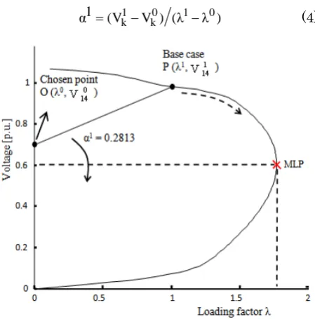
where α is the angular coefficient of the line. As a new equation is added, λ can be treated as a dependent variable and α is considered as the continuation parameter. With the solution of the base case (θ1, V1, and λ1) obtained with a PF, calculate the value of α1 from the point O (λ0, Vk0) and their respective values obtained in the base case
P (λ1, Vk1), as shown in Figure 1.
1 0 1 0
k k
1
α =(V −V ) (λ λ )− (4)
Figure 1. Performance of the method for the IEEE 14-bus system: first line through a chosen point O (λ0, V0) in the λV plan
The nodal voltage angle of the k bus can also be used to trace the P-V curves, Figure 2, in this case the equations (3) and (4) becomes:
0 ) θ θ ( ( α α) λ, , , ( ) λ , , ( 0 k k 0 ) λ λ
W = − =
= − − V θ 0 V G θ (5) ) λ λ ( ) θ θ
( 0 1 0
k 1 k
1
α = − − (6)
Figure 2. Performance of the method for the IEEE 14-bus system: first line through a chosen point O (λ0, θ0) in the λV plan
So, once α1 is computed by (4) or (5), the method is used to trace the P-V curve and to compute the MLP by applying successive increments (∆α) to the continuation parameter α.
For α =α1 + ∆α, the solution of the new system of equations formed by (3) or (5) will provide a new operation point (θ2, V2 and λ2) corresponding to the intersection of the solution trajectory (curve λ-V or λ-θ) with the line whose new angular coefficient value (α1+∆α) was specified. For α =α1, the converged solution should provide λ=1.
By expanding (3) or (5) in the Taylor series up to the first order terms, considering the preset value of α, yields
∆ = ∆ − = ∆ ∂ ∂ − W α W G x J x x G J m ∆ ∆ ∆ λ λ λ (7)where x=[θT VT]T, Jm is the Jacobian matrix of method,
and Gλ corresponds to the partial derivatives of G with
respect to λ. ∆G and ∆W denote the respective function
mismatches of new system of equations. It should be noted that the mismatches would be equal to zero (or close to zero, e.g., below the adopted tolerance) for the base case PF solution. Thus, only ∆W will be different from zero due to the change in α, e.g., due to its ∆α decrease.
4.1. A general Procedure for Changing the
Set of Lines
For some buses, the voltage magnitude can remain constant along a wide portion of the P-V curve and so, it could not be used as parameter to obtain that part of curve. Besides, depending on the voltage magnitude of a bus k
(Vk) chosen as parameter, the Jm may also become
singular where the J of PF becomes singular. Thus, either another parameter Vk must be used, or change to another
parameter (λ, θk, or other) will be necessary. The problem
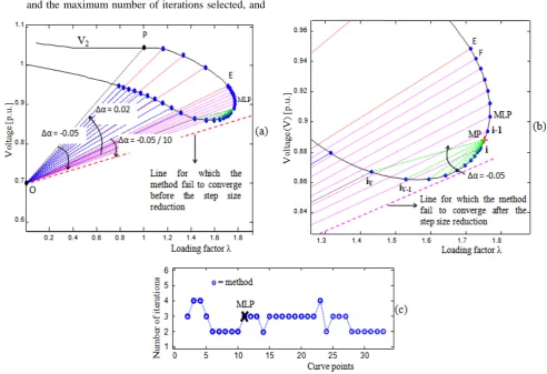
be used as parameter to obtain all the curve points. As a consequence of the difficulties presented during the choice of a continuation parameter from the set of bus voltage magnitudes, it was necessary to define a general procedure to choose the more appropriated set of lines to be used at each stage of the P-V curve tracing of system under study. After many tests, it was concluded that the following procedure is robust and also provides a low demand in terms of the total number of iterations needed to trace the P-V curves. Figure 3 is used to illustrate the general procedure, whose steps are:
1. Solve the base case (point P) using a PF method and compute points using a set of lines that passes through the initial chosen point O(λ0=0.0, V
k0=0.7
p.u.), labeled α0. The angular coefficient of the first line (α1) is computed by using (4);
2. Compute the next points of the P-V curve gradually changing the value of α, αi+1=αi+∆α, i.e., with a fixed step size (∆α) of, e.g., -0.05;
3. When the method fails to find a solution, return to the previous point (E), and then reduce the step size (e.g., divide by 10) considering the tolerance level and the maximum number of iterations selected, and
the mismatch criterion (details about the mismatch criterion will be presented afterwards);
4. When the method fails again (mismatch criterion), the parameter is changed to a set of lines, passing through midpoint MP((λi-1+λi)/2; (Vi-1+Vi)/2), see
details in Figure 3(b)) of the segment whose end points are the last two computed points: "i-1" (λi-1;
Vi-1) and "i" (λi; Vi). After that, compute the angular
coefficient of the first line considering the point MP and the last point "i". If λi>λi-1, then reduce the initial
step size (e.g., divide by 10); otherwise, it remains equal to its initial value. The inclusion of the midpoint is important to assure robustness, and helps the method to overcome singularities of J.
5. If ViV >ViV-1 (see detail in Figure 3(b)), then the
parameter is changed to a set oflines. After that, compute the angular coefficient of the next line considering the initial chosen point and the last point "iV". The step size could be increased to, e.g., +0.02
(note that the plus sign is due to the change in direction of the voltage magnitude, that is now increasing).
Figure 3. Performance of the method for the IEEE 14-bus system: (a) voltage magnitude at the generation bus 2 (V2) as function of λ, (b) detail of the MLP region, (c) number of iterations
The idea is the same when are used the equations (5) and (6), i.e., the λ-θplan to obtain the P-V curve.
The tracing of any desired P-V curve is carried out with the corresponding desired values of voltage magnitude and loading factor, which are stored during the procedure used for tracing the λ-θ curve.
4.2. Flowchart of the Method for the Tracing
of P-V curve
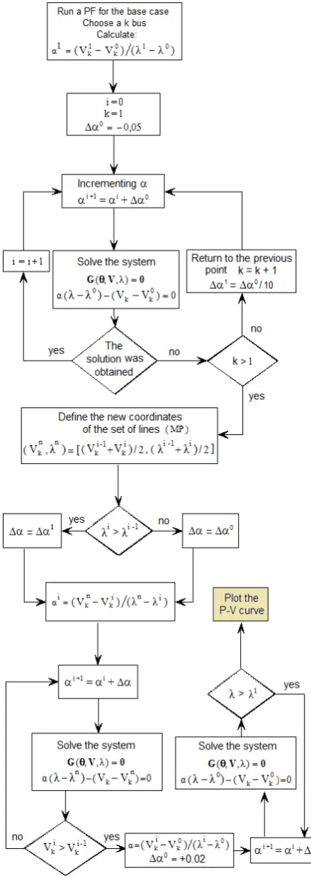
Figure 4. Flowchart of the method using the λ−V plan
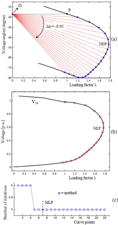
The flowchart of the proposed method utilizing the voltage angle of the k bus as the plan of tracing of the P-V curve can be seen in Figure 5. It may be observed that the flowchart was restricted only in the first set of lines, due to the fact that the voltage angles are decreasing during the loading margin of the system. Figure 6 shows the operation of the proposed method for tracing of the P-V curve using the flowchart of Figure 5. Figure 6(a) shows
the tracing of the λ−θ curve as plan for obtaining the P-V curve. Figure 6(b) presents the P-V curve of the critical bus 14 and the respective points stored by the proposed method. Figure 6(c) shows the number of iterations performed for obtaining each point. It can be concluded from these results that the inclusion of the parameterization switching procedure allows the complete tracing of the curve, with no ill-conditioning problems and still keeps a low number of iterations for most points.
Figure 5. Flowchart of the method using the λ-θ plan
4.3. The Choice of the Initial Point
Coordinates
value of the normal operation voltage range considered, in our case, smaller than 0.9 p.u. In general, the choice of voltage magnitude of the critical bus to compose the line equation make possible the whole P-V curve tracing without the need to change the coordinates of set of lines. However, in the base case, both the critical bus and the curvature of its solutions path are not known a priori. On the other hand, after many tests we verified that the voltage magnitudes of the critical buses of all analyzed power systems are around 0.7 p.u. So, the adoption of 0.7 p.u. for voltage magnitude and 0.0 for λ as the initial coordinates of the set of lines allows to trace the complete P-V curve and also, in general, led to better performance of the method. Using the nodal voltage angle to compose the line equation, the coordinates of point O (λ0, 0
k
θ ) will be the same as the base case P (λ1, 1
k
θ ), i.e., 0 k
θ =θ1k.
Figure 6. Performance of the proposed method for the IEEE 14-bus system: (a) voltage angle at the critical bus 14 (V14) as function of λ, (b) points of P-V curve stored by the proposed method, (c) number of iterations
4.4. The Mismatch Criterion
It is important to remember that the convergence criterion adopted to change the step size and parameters
during iterative process are the number of iterations, and the total mismatch criterion. The total mismatch is defined as the sum of the absolute values of the real and reactive power mismatches.
Figure 7. Convergence patterns of the PCPF at different P-V curve points: (a) for point "E", (b) for the next point of point "E" and keeping the step size of -0,05, (c) for point "b" after a step size reduction, (d) for the next point of point "b" with a maximum number of iterations of 20, (e) for the next point of point "b" with a maximum number of iterations of 25
In most cases the parameterizations result in a fast convergence, but in some cases this not occurs. The ill-conditioning cases can be identified by the mismatches
evolution. Figure 7(a) and Figure 7(b) show the total
process is divergent. As illustrated in Figure 3(a), the process failed in this case because the dashed line, whose angular coefficient is α =α+ ∆α, does not intersect the P-V curve, and the problem presents no solution. Returning to the previous point "E", and considering a step size reduction (∆α=∆α/10), the problem again presents solution and the next point "F" is obtained. Continuing the P-V curve tracing, the method fails again for the first point after the point "i" was obtained, as can be seen from the detail in Figure 3(b).
The total mismatch values corresponding to the iterative processes of point "i" and the next point (dashed line) are presented in Figure 7(c) and Figure 7(d). Note from the
mismatch evolution of point "i" in Figure 7(c), that the iterative process converged in 3 iterations, while for the next point (dashed line, after the step size of -0.005 in the value of α), the process does not diverge, but presents an oscillatory behavior. Despite the maximum value reduces gradually, it increases again after 22 iterations (see Figure 7(e)). Once again, as confirmed by the detail shown in Figure 3(b), the problem again presents no solution, because there is no intersection between the line and the P-V curve.
Based on these analyses, one can conclude that after the fourth iteration it is possible to detect such behavior. Thus, it was adopted as criterion, after the fourth iteration, to compare the last two values of total mismatch. If the last value is less than the previous one, the process continues to iterate; otherwise it stops and restarts from the previous point of the P-V curve. For the first divergence, the P-V curve tracing is made with a step size reduction. For the second divergence, it is made a change to a new set of lines, to the median point between the two last solutions computed (see Figure 3(b)).
This procedure avoids an excessive step size reduction and an overall large number of iterations during the tracing process. The switching to a new set of lines always occurred to a number of iterations less than the maximum number of iterations adopted (ten). For example, for the IEEE 14-bus it takes only six iterations to reduce the step size and to switch to a new set of lines. For the IEEE 30-bus, it takes only seven iterations.
5. Conclusion
This paper presented a parameterization schemes that allow the complete tracing of the P-V curves, i.e., complete tracing the correspondent P-V curve of each contingency (post-contingency loading margin) based on simple modifications of Newton’s method. Besides the fact that it locally removes the singularity, it should be emphasized that the inherent characteristics of the conventional method are enhanced, and the region of convergence around the singular solution is enlarged. It was also shown that continuation and conventional methods can be switched during the tracing process to determine efficiently all the P-V curve points with few iterations.
It is also important to remember the inclusion of the analysis of the behavior of the total power mismatch in the criteria used by the method to reduce the step size and change coordinates of the center of the set of lines, which was previously based only on the maximum number of
iterations. It was shown that the evolution of mismatch
indicates the possibility of ill-conditioning. Using this analysis obtained a reducing of iterations, i.e., changes always occur before reaching the maximum number of iterations, thus proving more advantageous for the tracing of the P-V curve.
Acknowledgement
The authors are grateful to the financial support provided by CNPq.
References
[1] WSCC-Reactive Power Reserve Work Group (RRWG), "Final Report: Voltage Stability Criteria, Undervoltage Load Shedding Strategy, and Reactive Power Reserve Monitoring Methodology", 145 p. 1998.
[2] FTCT-Força Tarefa Colapso de Tensão. Critérios e Metodologias Estabelecidos no âmbito da Força - Tarefa Colapso de Tensão do GTAD/SCEL/GCOI para Estudos de Estabilidade de Tensão nos Sistemas Interligados Norte/Nordeste, Sul/Sudeste e Norte/Sul Brasileiros, XV SNPTEE, GAT-10, Foz do Iguaçu, PR, 1999. [3] Mansour Y. Suggested techniques for voltage stability analysis,
IEEE Power Engineering Subcommittee Report 93TH0620-5-PWR, 1993.
[4] Alves D.A., da Silva L.C.P., Castro C.A., and da Costa V.F. Parameterized fast decoupled power flow methods for obtaining the maximum loading point of power systems - part-I: mathematical modeling, Electr. Power Syst. Res. 69 (2004) 93-104.
[5] Cañizares C.A., Alvarado F.L. Point of collapse and continuation methods for large ac/dc systems, IEEE Trans. on Power Syst. 8 (1993) 1-8.
[6] Ajjarapu, V.; Christy, C. The Continuation Power Flow: a Tool for Steady State Voltage Stability Analysis. IEEE Trans. on Power Systems, v.7, n.1, p. 416-423, 1992.
[7] Chiang, H. D.; Flueck, A.; Shah, K.S.; Balu, N. CPFLOW: A Practical Tool for Tracing Power System Steady State Stationary Behavior Due to Load and Generation Variations. IEEE Trans. on Power Systems, v.10, n.2, p. 623-634, 1995.
[8] Seydel, R. From Equilibrium to Chaos: Practical Bifurcation and Stability Analysis. 2ª ed. New York: Springer-Verlag, 407p, 1994. [9] Magalhães, E. M.; Bonini Neto, A.; Alves, D. A.. A
Parameterization Technique for the Continuation Power Flow Developed from the Analysis of Power Flow Curves. Mathematical Problems in Engineering, v. 2012, p. 1-24, 2012. [10] Bonini Neto, A.; Alves, D. A. Improved Geometric
Parameterization Techniques for Continuation Power Flow. IET Generation, Transmission & Distribution, v. 4, p. 1349-1359, 2010. [11] IEEE Power System Stability Committee, Special Publication, Voltage Stability Assessment, Procedures and Guides, Final Draft, 1999. [Online]. Available: http://www.power.uwaterloo.ca. [12] Reactive Power Reserve Work Group. Voltage Stability Criteria,
Undervoltage Load Shedding Strategy, and Reactive Power Reserve Monitoring Methodology, (1998) p. 154, Available: http://www.wecc.biz/library/Documentation Categorization Files/Guidelines (File name: Voltage Stability Criteria – Guideline, Date adopted/approved April 2010).
[13] ONS Operador Nacional do Sistema Elétrico, "Procedimentos de Rede Submódulo 23.3, Diretrizes e Critérios para Estudos Elétricos", 2002.
[14] Bonini Neto, A.; Alves, D. A. An improved parameterization technique for the Continuation Power Flow. In: Transmission and Distribution Conference and Exposition, IEEE PES, 2010, New Orleans, LA, USA. p. 1-6.