Vol 7, No 6 (2017)

Computer Science and Software Engineering

ISSN: 2277-128X (Volume-7, Issue-6)

2017

Similarity Solution of Non-Linear Boussinesq’s Equation

Arising in Infiltration of Incompressible Fluid Flow

N. B. Desai

Department of Mathematics, A. D. Patel Institute of Technology, New V. V. Nagar-388 121, India

DOI: 10.23956/ijarcsse/V7I6/0202

Abstract: Infiltration of ground water on the ground water surface has been modeled in the form of non-linear Boussinesq’s equation. The solution of the governing equation in height of the mound and time t and distance has been obtained by using Lie –group scaling transformation, we determined the similarity solution. After the introduction of the similarity variables, problem is reduced to ordinary nonlinear fractional differential equation. Exact solutions to ordinary fractional differential equation, which is derived from the non-linear Boussinesq’s equation, is presented

Keywords: Infiltration, water mound, Similarity Solution, Non-linear Boussinesq’s equation.

I. INTRODUCTION

Ground water is extremely important to our way of life. Most drinking water supplies and often irrigation water for agricultural needs are drawn from underground sources. More than 90% of the liquid fresh water available on or near earth’s surface is groundwater. Groundwater is derived from rain and melting snow that percolate downward from the surface; and collected in the open pore spaces between soil particles or in cracks and fissures in bedrock. The process of percolation is called infiltration.

Infiltration is the process by which water on the ground surface enters the soil. Infiltration rate in soil science is a measure of the rate at which soil is able to absorb rainfall or irrigation. It is measured in inches per hour or millimeters per hour. The rate decreases as the soil becomes saturated. If the precipitation rate exceeds the infiltration rate, runoff will usually occur unless there is some physical barrier. It is related to the saturated hydraulic conductivity of the near-surface soil.

Infiltration is governed by two forces: gravity and capillary action. While smaller pores offer greater resistance to gravity, very small pores pull water through capillary action in addition to and even against the force of gravity. The rate of infiltration is affected by soil characteristics including ease of entry, storage capacity, and transmission rate through the soil. The soil texture and structure, vegetation types and cover, water content of the soil, soil temperature, and rainfall intensity all play a role in controlling infiltration rate and capacity. For example, coarse-grained sandy soils have large spaces between each grain and allow water to infiltrate quickly. Vegetation creates more porous soils by both protecting the soil from pounding rainfall, which can close natural gaps between soil particles, and loosening soil through root action. This is why forested areas have the highest infiltration rates of any vegetative types.

The top layer of leaf litter that is not decomposed protects the soil from the pounding action of rain, without this the soil can become far less permeable. In chaparral vegetated areas, the hydrophobic oils in the succulent leaves can be spread over the soil surface with fire, creating large areas of hydrophobic soil. Other conditions that can lower infiltration rates or block them include dry plant litter that resists re-wetting, or frost. If soil is saturated at the time of an intense freezing period, the soil can become a concrete frost on which almost no infiltration would occur. Over an entire watershed, there are likely to be gaps in the concrete frost or hydrophobic soil where water can infiltrate.

Once water has infiltrated the soil it remains in the soil, percolates down to the ground water table, or becomes part of the subsurface runoff process. The process of infiltration can continue only if there is room available for additional water at the soil surface. The available volume for additional water in the soil depends on the porosity of the soil and the rate at which previously infiltrated water can move away from the surface through the soil. The maximum rate that water can enter a soil in a given condition is the infiltration capacity. If the arrival of the water at the soil surface is less than the infiltration capacity, all of the water will infiltrate. If rainfall intensity at the soil surface occurs at a rate that exceeds the infiltration capacity, pounding begins and is followed by runoff over the ground surface, once depression storage is filled. This runoff is called Horton overland flow. The entire hydrologic system of a watershed is sometimes analyzed using hydrology transport models, mathematical models that consider infiltration, runoff and channel flow to predict river flow rates and stream water quality.

unsaturated porous media. (Mehta and Desai (2010)) discussed the solution of seepage of ground water in soil by Homotopy perturbation method. (Mehta and Patel (2008)) discussed solution of Burger’s equation arising into the one dimensional ground water recharge by spreading in porous media. (Mehta and Meher (2010)) discussed the Adomian decomposition method for moisture content in one dimensional fluid flow through unsaturated porous media. (Mehta and Yadav (2008)) discussed the solution of problem arising during vertical ground water recharge by spreading in slightly saturated porous media. (Joshi and Mehta (2010)) apply the Group theoretic approach to the problem of one dimensional fluid flow through unsaturated porous method.

II. STATEMENT OF THE PROBLEM

Assume that Ground water infiltration take place over large basin area, it enters soil and achieve some water table. The problem is to determine effective height of the water table as measure of the initial storage capacity of the basin. In order to obtain the governing equation of infiltration we make the following assumptions.

a) The stratum has height

h

_mand lies on the top of horizontal impervious bed which we label as

z



0

. b) We ignore the transversal variable y and

c) The water mass which infiltrates the soil occupies a region described as

 



 

x z

,



R z



h x t

 

,



and hence we assume that there is no partial saturation.

Where

h x t

 

,

is called the free boundary function and it determine the height of the free surface. Also

0



h x t

 

,



h

_m, where,

h

_m is the maximum height of the free surface. In this situation we arrive at system of three equations in three unknowns; two velocity components

u and v

and pressure

p

in a variable domain.

 Equation of mass conservation for an incompressible fluid.

 Two equations of mass conservation of momentum of the Navier stoke type.

The resulting system of equations with initial and boundary conditions is too complicated and in order to simplify the equation, we make the following additional assumptions.

We assume that the flow is horizontal, i.e.

V

 

u

, 0





and the free boundary function

h x t

 

,

has small gradients. The momentum equation in vertical component

 

u

z is given by,

.

z

z

du

p

v u

g

dt

z





_

 



_

 













(1)

Neglecting the LHS term of (1), and integrating with respect to z, we obtain

tan C

p





gh



cons

t

(2)

If we impose the continuity of the pressure across the interface and assuming the constant atmospheric pressure in the air that fills the pore of the dry region

z



h x t

 

,

and letting

p



0

on the free surface

z



h x t

 

,

in equation (2) gives us,



gh



cons

tan C

t

(3)

Hence from (2) and (3) we obtain,





p





g h



z

(4)

In other words, the pressure is determined by the hydrostatic approximation.

Considering the mass conservation law for a section

S





x x a

,

 

 

0,

C



, we get

0 x a h

x S

dydx

V n dl

t



 









_{ }



_













_

 

_







(5)

Where



is the porosity of the medium (i.e. fraction of the volume available for flow circulation),

V



is the velocity, which obeys the Darcy’s law form which includes the gravity effects.

V

k



p



gz







  



(6)

Considering the velocity component of

V



along the lateral surface (i.e.

V n

u



 

), we obtain

k

p

u

x





 



(7)

k

h

u

x





 



(8)

Inserting the expression of u in the equation (5), we obtain

0 h

h

gk

hdz

t

x

x























_

_

_



_



_

_



_





_

(9)

Hence the above equation (9) in the form of non-linear Boussinesq equation is given by,

2 2 2

;

2

h

gk

h

where

t

x











_

_{  }

_

 





(10)

The above equation (10) gives the height of the water table at any distance x and at any time t. Using the dimensionless variables

T

gk

t and X

x

L











_

_







, the equation (10) simplifies to

h

h

h

T

X

X



_























(11)

The appropriate initial and boundary conditions are given by





 

0

0

, 0 F X 0 0, 0 1

h X at T and X h

h

     (12a)

 

1,

 

1 &

0

h

T

 

H G T at X



T



(12b)

Another generalization of (11) was proposed by Mainardi See[12,8] In Mainardi approach, the integer-order derivative is replaced by a fractional derivative, so that (11) becomes

α

α

h

h

=

h

T

X

X

























(13)

Where α α

h

T





is used to denote the left Riemann-Liouville fractiolnal derivative of order

α

with respect to time T. For

any

0

 

α 1

and an absolutely continuous function

f(t)

, the left fractional derivative of the order

α

is defined as

T α α α 0 T (1) α α 0

d f

d

1

f(τ)

=

dτ

dT

dT Γ(1-α)

(T-τ)

1

f(0)

f

(τ)

=

+

dτ

Γ(1-α) T

(t-τ)

















(14)

Where



is the Euler Gamma function. Higher order fractional derivatives are defined similarly. Thus , if





and

1

p

  



p

where

p

is an integer,then

β

β

d f

dt

is defined as

In this paper we shall treat the generalization of (13) corresponding to the case when

h= k+mh



_

n



_

with k, m and n being given constant. With this value (13) becomes,





α n α h h = k+mh

T X X

    

 

     (15)

In (15) we shall assume that k>0.

III. SIMILARITY TRANSFORMATION

In order to prove that equation (15) possesses similarity solutions, we will first perform its lie group scaling transformation

We will transform (15) by introducing new independent and dependent variables denoted by

T,X,h

 



in the following way:

T= T X=







p

X h=





q

h(X,T)



 

(16)

Where p and q are parameters, which will be determined from the condition that (15) remains invariant under this transformations.

2

q q-2p q(1+n)-2p n

2

h h h

k m (h )

T X X X

If

k



0

,the condition of invariance obviously reads.

q- =q-2p=q(1+n)-2p



from which we get

q = 0, p

2





(17) If k=0 , the same condition simplifies, to:

q- =q(1+n)-2p



, yielding

2p-q=

, p

n



- arbitrary (18) Now we can eliminate



between the transformation formulas and get:

q p

1 1

P P

T

T

h

X

and

=

X

h

X

X

 



_{ }

 









This shows that h(X,T) can expresses as:

q _-1

p p

h=X

U(X T)

,

Where U is a function of the combination of independent variables,

-1 p

X T

alone satisfying an ordinary differential equation. This actually means that equation (15) possesses similarity solutions of the form:





a b

h X,T =X U(ξ) ξ=X T

(19)

Where a and b are constants, to be determined by (17) or (18).Namely, if

k



0

we have a = 0,

b=

-2



and if k=0,

(an-2)

b=



while a remains arbitrary. In order to derive the ordinary differential equation for we will be in need of the

following formulas.

T

0

ξ a bα

b -b

α 0

h

1

h(X, )

d

T

(1

) T

(t

)

1

d

X U(y)X

=

x

X dy

(1

)

dξ

(ξ-y)

  



_









_





 





 





(20)

Where

y=X

b



from (16) we obtain

a+b

h

d U(ξ)

X

T

dξ

    



_



(21)

Similarly we have

a-1 a b-1 a-1

1

h

dU(ξ)

=aX U(ξ)+X

bX T=X F (ξ)

X

dξ





1

dU(ξ)

F (ξ)=aU(ξ)+bξ

dξ

2 a-2 2 2

h

=X F (ξ)

X





1 2 1 2 2 2 2

dF (ξ)

F (ξ)=(a-1)F (ξ)+bξ

dξ

dU(ξ)

d U(ξ)

=a(a-1)U(ξ)+b(2a+b-1)ξ

+b ξ

dξ

dξ





n a(1+n)-2

n

h

dF(ξ)

h

= X

a(1+n)-1 F+bξ

X

X

dξ

dU(ξ)

From (19) and by substituting (21) and (22) in (13) we obtain

For the nonlinear fractional equation (13) the similarity solution has the form

a b

h(X,T)=X U(ξ) ξ=X T

(23)

-2

where a=0 ,b=

, for k

0

an-2

b=

,a arbitrary for k = 0

α





(24)

Also is a solution to the following ordinary nonlinear fractional equation





2 2 2

2

n

d U(ξ)

dU(ξ)

d U(ξ)

a(a-1)U(ξ)+b(2a+b-1)ξ

+b ξ

dξ

dξ

dξ

dF(ξ)

+m

a(1+n)-1 F+bξ

dξ

dU(ξ)

Where F= U

aU+bξ

dξ

k









 































(25)

IV. EXACT SOLUTIONS

We will now show how some exact solutions to the equation (25) can be found. First we will suppose that k = 0 in (13) and seek the exact solution in the following form.

β 1

U=U ξ

(26)

Where

U

1 and

β

are constants. Then, it is readily shown that the left-hand side of (25) transforms for

β>-1

into β-α

1

U β(1-α,1+β)

(1-α+β)ξ

,

Γ(1-α)

where

1

v-1 w-1

0

β(v,w)= u (1-u) du



is beta function with parameter v and w, while the right –hand side becomes





n+1 (n+1)β

1

m(a+bβ)(U )

a(1+n)-1+bβ(n+1) ξ

Obviously, (26) can be a solution to (25) when:

β=

-α

,n>α

n

only. Equating the coefficients in front of the same power

on both sides of (25), respecting (24) and using some elementary properties of Beta and Gamma functions, we obtain the following expression for the coefficient

U

₁

1 n 2

1

α

n Γ(1-

)

n

U =

α

2m(2+n)Γ(1-α-

)

n

















(27)

At that, a is eliminated and does not effect the final result. Inserting (26) into (19) we also get a result that does not depend on a i.e

2 n

1 α

2

X

h(X,T)=U

T













(28)

Thus (27) and (28) hold for a=0 also.

Since a = 0 indicates

k



0

it is natural to try to find an exact solution of (25) for the case

k



0

again in the form (26). Thus, assuming a possible solution to (25) with

k



0

in the form (26) one can easily verify that it exists for n = 2. The values of the constants and are simply obtained from their corresponding values for by inserting there n = 2. This also holds for the final solution of (11) in the form (28).

Another exact solution of (11) has the form of a wave propagating along the X-axis with certain speed c and cannot be obtained from (25). To get this solution another similarity transformation of (13) has to be performed for k = 0 It reads

a

cT

h=X U(ξ) , ξ=

-1

X

(29)

ξ α a-α

α -1

c X

d

U(η)

dη

Γ(1-α) dξ (ξ-η)



While the right-hand side becomes





(n+1)a-2

n

dF

mX

(n+1)a-1 F-(1+ξ)

dξ

dU

where F(ξ)=U

aU-(1+ξ)

dξ

























Obviously, the condition for the existence of this similarity solution is

a-α = (n+1)a - 2 ,

2-α

giving a =

n

(30)

The ordinary fractional – order differential equation to which (13) reduces to is





ξ α

α -1

c

d

U(η)

dF

dη=m

(n+1)a-1 F-(1+ξ)

Γ(1-α) dξ (ξ-η)

dξ















(31)

We seek the solution of this equation in the following form

1

,

0 (

)

( )

0 ,

0 (

),

U

X

cT

U

X

cT

















 







(32)

Where

U

₁ is constant. Proceeding as in the case of the previous exact solution, we can show that, after the use of (32) equation (31) is transformed to





α β-α n+1 (n+1)β n+1 (n+1)β-1

1 1 1

n+1 1

Γ(1+β)

U c

(1-α+β)ξ

=m(U ) (α-β) (n+1)(α-β)-1 ξ

-2m(U ) β(n+1)(α-β)ξ

Γ(2-α+β)

+m(U )

β (n+1)β-



1 ξ



(n+1)β-2

We can satisfy this equation by the unique choice

2-α

β=α=

n

That provides 1 n α 1 2-α nc Γ 1+

n = 2-α m(2-α)Γ 2-α+ n U              _{ }  _{ }  _{ }   (33)

Then the final solution (28) reads

2-α n 1

h(X,T)=U (cT-X)

, X



cT

(34) We can solve (33) for c to obtain

1

n 1

2-α

m(U ) (2-α)Γ 2-α+

n

c=

2-α

nΓ 1+

n





















_

_





_

_





_

_















(35)

By using (35) in (34) we finally obtain

2 1 n 1 1

2-α

m(U ) (2-α)Γ 2-α+

It is to be noted that in the literature there are no known relation of this type for fully nonlinear problems in porous media for





1

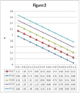
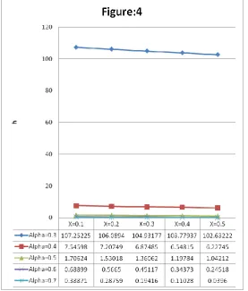
our results match.

In Figs. 1-3 we plot 36 for the special case





0

.

5

,

m



1,

U

₁



1

and different value of n and T.

Figure :1 for





0

.

5

,

m



1,

U

₁



1

, n=1 and different value of T.

Figure :3 for





0

.

5

,

m



1,

U

₁



1

, n=2.0 and different value of T. Further increase in n to the value n=2 as shown in figure 3 it is seen that for

n



1

.

5

becomes concave Next we are examining the effect of the parameter



for the fixed time instant.

Again by decreasing the order of the derivatives that is



decrease the graph changes from concave to convex.

V. CONCLUSIONS

In this paper we studied fractional nonlinear heat conduction equation by the use of similarity transformations. The generalization is obtained by replacing integer-order derivative by fractional derivative (more precisely, derivative of real order).We show in the paper that the fractional nonlinear partial differential equations studied possess similarity solutions, exactly as their counterparts with integer-order derivatives. By using conveniently defined similarity variables these partial differential equations reduce to ordinary differential equations with fractional-order derivatives, which are more amenable to various analytical and numerical techniques.

REFERENCES

[1] Bear, J.,“Dynamics of fluids in porous media”, American Elsevier Publishing Company, Inc., 1972

[2] Brailovsky, I., Babchin, A., Frankel, M., and Sivashinsky, G., “Fingering instability in water-oil displacement”, Transport in Porous Media, Vol. 63, Issue3, pp. 363-380, 2006.

[3] D.D. Joseph, L. Preziosi, Heat waves, Rev. Modern Phys. 61 (1989) 41–73.

[4] Desai, N. B.,“The study of problems arises in single phase and multiphase flow through porous media”, Ph.D. Thesis, South Gujarat University, Surat, 2002.

[5] D.V. Widder, The Heat Equation, Academic Press, New York, 1975

[6] G.W. Bluman, S. Kumei, Symmetries and Differential Equations, Springer, Berlin, 1989.

[7] Hansen A G. similarity analysis of boundary value problems in engineering: Prentice Hall of Canada, LTD. Canada:02.

[8] I. Podlubny, Fractional Differential Equations, Academic Press, San Diego, 1999.

[9] M. Abramowitz, I.A. Stegun, Handbook of Mathematical Functions, Dover, New York, 1965.

[10] Mehta M. N., “Asymptotic expansions of fluid flow through porous media”, Ph. D Thesis, South Gujarat University, Surat, India, 1977

[11] Mehta, M. N., and Joshi, M. S., “Solution by group invariant method of instability phenomenon arising in fluid flow through porous media”, Int. J. of Engg. Research and Industrial App., Vol. 2, No. 1, pp. 35-48, 2009. [12] Mehta M. N. and Saroj Yadav” Classical solution of Non-linear Equation arising in fluid flow through

Homogeneous Porous Media” , SVNIT,Surat,2009.

[13] Mehta M N.and Meher S K “Adomian decomposition method for moisture content in one dimensional fluid flow through unsaturated porous media”. IJAMM.6(7), 13-23,2010.

[14] Mukherjee, B., and Shome, P., “An analytic solution of fingering phenomenon arising in fluid flow through porous media by using techniques of calculus of variation and similarity theory”, Journal of Mathematics Research, Vol. 1, No. 2, 2009.

[15] N.H. Ibragimov (Ed.), CRC Handbook of Lie Group Analysis of Differential Equations, vol. I–III, CRC Press, 1994.

[16] Patel and Mehta ”Burger Equation arising in problems of fluid flow through porous media”. Ph.D. Thesis.SVNIT Surat,2007.

[17] P.J. Olver, Application of Lie groups to Differential Equations, Springer, Berlin, 1986.

[18] Polubarinova-Kochina P. Ya. Theory of Groundwater movement, Princeton University Press 1962. [19] R. Hilfer (Ed.), Applications of Fractional Calculus in Physics, World Scientific, Singapore, 2000. [20] Scheidegger, A. E.,“The Physics of flow through porous media”, Soil Science, Vol. 86, 1958

[21] Scheidegger, A. E., and Johnson, E. F.,“The statistically behaviour of instabilities in displacement process in porous media”, Canadian J. Physics, Vol. 39, Issue 2, pp. 326-334,1961

[22] T.M. Atanackovic, B. Stankovic, “An expansion formula for fractional derivatives and its applications” Fract. Calculus Appl. Anal. 7 (3) (2004) 365–378.

[23] T. Ozer, “On symmetry group properties and general similarity forms of the Benney equations in the Lagrangian variables”, J. Comput. Appl.Math. 169 (2004) 297–313.

[24] Tullis, B. P., and Wright, S. J.,“Wetting front instabilities: a three dimensional experimental investigation”, Transport in Porous Media, Vol. 70, pp. 335–353, 2007