Proceedings of the Workshop on the
Layout of (Software) Engineering Diagrams
(LED 2007)
Logichart: A Prolog Program Diagram and its Layout
Yoshihiro Adachi and Yudai Furusawa
16 pages
Guest Editors: Andrew Fish, Alexander Knapp, Harald St ¨orrle
Managing Editors: Tiziana Margaria, Julia Padberg, Gabriele Taentzer
Logichart: A Prolog Program Diagram and its Layout
Yoshihiro Adachi1and Yudai Furusawa2
1[email protected] 2[email protected]
Department of Information and Computer Sciences Toyo University at Kawagoe, Japan
Abstract:The layout of Logichart diagrams is first discussed. The layout condition is formalized with a layout constraint (expressions of equalities and inequalities) of tree-structured diagrams. Next, a cell placement that gives the minimum-area layout under a specific layout constraint is presented. A Logichart attribute graph grammar is then formalized. This grammar is underlain by a neighborhood controlled embed-ding (NCE) graph grammar whose productions are defined in order to formalize the graph-syntax rules of Logichart diagrams. Semantic rules attached to the grammar’s productions are defined in such a way that they can extract the layout information needed to display a Logichart diagram by means of the attributes attached to the nodes of the graphs derived by the grammar. The semantic rules are formalized so as to obtain the Logichart diagrams of the minimum area under the above layout constraint.
Keywords:Prolog program diagrams, Attribute graph grammar, Graph layout
1
Introduction
Visualization using program diagrams can effectively facilitate the understanding, debugging, and education of programs. The Transparent Prolog Machine, a well-known Prolog visualization system [1,2], displays the structure of a pure Prolog program as a tree with AND/OR branches (an AND/OR tree) and depicts the states of the various goals as symbols at its nodes. Other Prolog visualization and debugging systems, e.g., [3], also deal primarily with pure Prolog and use AND/OR trees. However, it is not easy to correlate the content of a Prolog program with that of its corresponding AND/OR tree, because the structure of the clauses of the Prolog program, and their representations in the AND/OR tree, are different.
prolog_program test(X,Y,Z)
test(X,Y,Z)
test(_, _, _)
appendList(X, Y, Z)
appendList([], X, X) appendList([X|L1], L2, [X|List]) appendList(L1, L2, List)
appendList([X|L1], L2, [X|List])
write((X, Y, Z))
write(end)
nl
appendList([], X, X)
nl
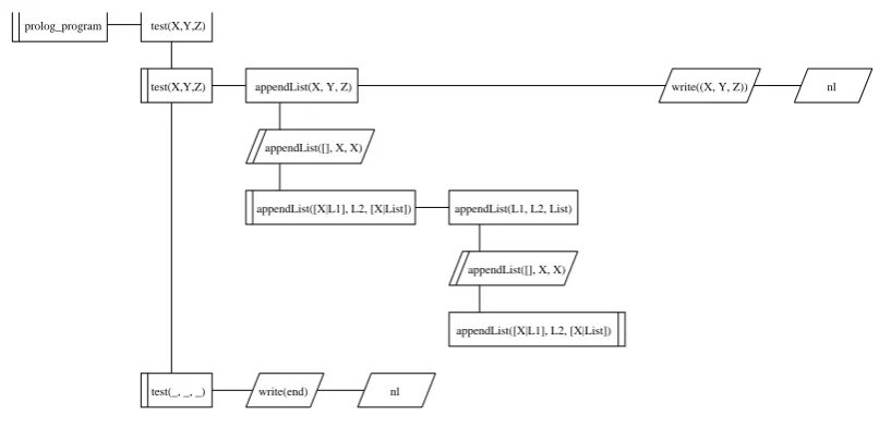
Figure 1: Example of Logichart diagrams
In this paper, we first explain the structure of Logichart diagrams and discuss their layout. The layout condition is formalized with a layout constraint (expressions of equalities and inequalities) of tree-structured diagrams. We then present a cell placement that gives the minimum-area layout of a Logichart diagram under a specific layout constraint.
A Logichart diagram has a graph structure composed of nodes (which are called cells in Logichart) and edges. The syntax rules of Logichart diagrams are therefore well formalized with a graph grammar. Furthermore, layout information (the x- and y-coordinates of each node) can be well evaluated by means of attributes attached to each node label and layout rules attached to each production of the graph grammar. Based on these viewpoints, we formalize the syntax and layout rules of Logichart diagrams based on an attribute graph grammar [6, 7], and as a result, we define the Logichart attribute graph grammar (Logichart-AGG for short). This gram-mar is underlain by a neighborhood controlled embedding (NCE) graph gramgram-mar that generates ordered graphs [8]. Its productions are defined in order to formalize the graph-syntax rules of Logichart diagrams, and the semantic rules attached to the grammar’s productions are defined in such a way that they can extract the layout information needed to display a Logichart diagram by means of the attributes attached to the nodes of the graphs derived by the grammar. The semantic rules are formalized so as to obtain Logichart diagrams of the minimum area under the above layout constraint.
2
Prolog program visualization
2.1 Logichart diagrams
Prolog is generally an interpreted language, although compiler implementations do exist. A
Prolog program consists of a set of clauses. Each clause has a head and a body. The body
consists of either no goals, one goal, or a sequence of goals. A Prolog program is executed when the interpreter is given a query that consists of one or more goals. The system uses its computation rule to select a goal from the query, then uses its search rule to search for a clause whose head matches the goal. If such a clause is found and called, the current query becomes (is reduced to) a new query by replacing the selected goal with the body that corresponds to the matching head. The Prolog system dynamically constructs the execution of its programs (queries) in this way.
Logichart diagrams have been developed to represent computation, which is the response of a Prolog program to a query, as an intelligible diagram [4]. A Logichart diagram is relatively easy to understand, and correspondence with the source Prolog program is clearly presented. Figure1 shows a Logichart diagram that corresponds to the Prolog program shown below and the query ‘?- test(X,Y,Z).’.
test(X,Y,Z) :- appendList(X,Y,Z), write((X,Y,Z)),nl.
test(_,_,_) :- write(end),nl. appendList([],X,X).
appendList([X|L1],L2,[X|List]) :-appendList(L1,L2,List).
2.2 Drawing constraints of Logichart diagrams
Drawing Logichart diagrams requires their cells to be laid out. This section discusses the layout conditions for Logichart diagrams.
A Logichart diagram has a rooted, binary tree structure. The layout conditions of Logichart diagrams are formalized as the layout constraints of tree-structured diagrams as follows.
Definition 1 AnL-tree-structure T is defined byT = (V,E,r,LE,width,depth), where(V,E) is abinary tree,V is a set ofcells,E is a set ofedgesand therootcell isr∈V. LE:E→ {h,v} is an edge labeling function. The mapwidth:V →Ris thewidth f unctionof the cells, and the mapdepth:V →Ris thedepth f unctionof the cells.
The horizontal length is represented bywidth(p), which is called thewidth o f cell p, and the vertical length is represented bydepth(p), which is called thedepth o f cell p.
Definition 3 LetT = (V,E,r,LE,width,depth)be an L-tree-structure andπ be the placement
ofT:D= (T,π)is called anL-tree-structured diagram(L-TSD for short).
L-TSDs are drawn by mapping each cell to a set of planar coordinates and joining the cells to-gether with line segments corresponding to each edge. The x- and y-coordinates are taken along the respective horizontal and vertical directions, and the coordinates of each cell are considered to be those of its top left corner.
Definition 4 LetT = (V,E,r,LE,width,depth) be an L-tree-structure,π be the placement of
T, and D= (T,π) be an L-TSD. Thewidthand the depth o f Dare defined by the following
functions:
width(D) ≡ max{|πx(p) +width(p)−πx(q)|:∀p,q∈V}.
depth(D) ≡ max{|πy(p) +depth(p)−πy(q)|:∀p,q∈V}.
Definition 5 LetT = (V,E,r,LE,width,depth) be an L-tree-structure,π be the placement of
T, andD= (T,π)be an L-TSD. Thearea o f Dis defined as
area(D)≡width(D)×depth(D).
For cellss andt of an L-TSD,t is called av-child ofsif there is an edge labeled vfroms
tot. Similarly, t is called an h-child ofs if there is an edge labeledh froms tot. Here,t is called av-descendantofsif there is a path composed of edges labeledv. Similarly,t is called anh-descendantofsif there is a path composed of edges labeledh.
Here, v-subTSD with root cells is defined as a subdiagram of an L-TSD consisting of cell
s, itsv-childt, an edge labeledvfromstot, and a subTSD of the L-TSD whose root cell ist. Similarly,h-subTSD with root cellsis defined as a subdiagram of an L-TSD consisting of cells, itsh-childt, an edge labeledhfromstot, and a subTSD of the L-TSD whose root cell ist. The
sitself is theh-subTSD with root cellsifshas noh-child. A cell with no input edge labeledhis called ahead cell, and a cell with an input edge labeledhis called agoal cell.
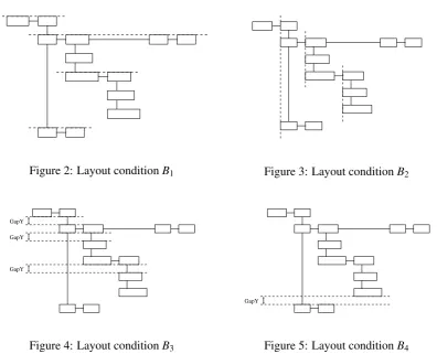
An edge labeled h is drawn horizontally, and an edge labeled v is drawn vertically for an
L-TSD. The layout constraints for drawing L-TSDs are as follows.
ConditionB1: Iftis anh-child ofs, then
πy(s)=πy(t). (Figure 2)
ConditionB2: Iftis av-child ofs, then
πx(s)=πx(t). (Figure 3)
ConditionB3: Ifsis a goal cell, then
πy(v-child ofs)≥πy(s)+depth(s)+ GapY. (Figure 4)
ConditionB4: Ifsis a head cell, then
πy(v-child ofs)≥max{πy(t) +depth(t)|tis a cell ofh-subTSD ofs}+ GapY. (Figure 5)
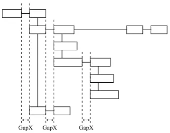
ConditionB5: Ifsis a goal cell, then
ConditionB6: Ifsis a head cell, then
πx(h-child ofs)≥πx(s)+width(s)+ GapX. (Figure 7)
Figure 2: Layout conditionB1 Figure 3: Layout conditionB2
GapY GapY
GapY
Figure 4: Layout conditionB3
GapY
Figure 5: Layout conditionB4
The minimum-area L-TSD is obtained with the following theorem.
Theorem 1 For any L-TSD, the placement,π, satisfying the condition, C1∧C2∧C3∧C4∧C5∧
C6, gives the minimum-area L-TSD satisfying B1∧B2∧B3∧B4∧B5∧B6.
ConditionC1: If t is an h-child of s, then
πy(s)=πy(t).
ConditionC2: If t is a v-child of s, then
πx(s)=πx(t).
ConditionC3: If s is a goal cell, then
πy(v-child of s) =πy(s)+ depth(s)+ GapY.
ConditionC4: If s is a head cell, then
πy(v-child of s) = max{πy(t) +depth(t)|t is a cell of h-subTSD of s}+ GapY.
ConditionC5: If s is a goal cell, then
GapX GapX
Figure 6: Layout conditionB5
GapX
GapX GapX
Figure 7: Layout conditionB6
ConditionC6: If s is a head cell, then
πx(h-child of s) =πx(s)+ width(s)+ GapX.
Proof. It is obvious thatC1∧C2∧C3∧C4∧C5∧C6impliesB1∧B2∧B3∧B4∧B5∧B6. Suppose a placement, πC, satisfiesC1∧C2∧C3∧C4∧C5∧C6. For L-TSD under the placement, πC, cells connected with an edge labeledhcannot be placed closer because of the layout conditions,
B2∧B5∧B6. Thus, the placement,πC, gives the layout with the minimum width. Similarly, for L-TSD under the placement,πC, cells connected with an edge labeledvcannot be placed closer because of the layout conditions,B1∧B3∧B4. Thus, the placement,πC, gives the layout with the minimum depth. Consequently, the placement,πC, gives the layout with the minimum area.
Drawing binary trees that only have rightward-horizontal and downward-vertical segments is known ash-v drawing. Several studies on h-v drawing problems have been presented [10,11]. The L-TSD drawing problem differs from these because an L-TSD’s cells have a particular size (height and depth), and its layout constraints also differ from theirs.
3
Logichart-AGG
The Logichart-AGG consists of an edNCE graph grammar that generates ordered graphs and semantic rules. The edNCE grammar has formalized productions that specify the syntax rules of Logichart diagrams, and the semantic rules enable us to calculate the node coordinates of Logichart diagrams satisfying the layout constraints described in the previous section.
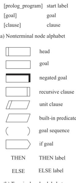
The Logichart-AGG specifications are very concise and consist of 13 productions associated
with 88 semantic rules. The node label alphabet of the Logichart-AGG is shown in Figure8.
The edge label alphabet isΓ=Ω={e,h,v}. We introduced additional edges labeled ‘h’ and ‘v’ to the Logichart-AGG in order to regard the diagrams derived by it as L-TSDs. A Logichart diagram is obtained by removing all edges labeled ‘h’ and ‘v’ from the diagram derived by the Logichart-AGG.
[prolog_program] start label [goal] goal [clause] clause (a) Nonterminal node alphabet
(b) Terminal node alphabet head
THEN
ELSE
goal
negated goal
recursive clause
if goal unit clause
built-in predicate
goal sequence
THEN label
ELSE label
Figure 8: Node alphabets of Logichart-AGG
Inherited attributes of node labels (except the initial label):
• πx: thex-coordinate of a node
• πy: they-coordinate of a node
Synthesized attributes of nonterminal node labels:
• subtree width : the width of a subtree
• subtree depth : the depth of a subtree
The following symbols and functions are used in the productions and semantic rules of the Logichart-AGG.
• <X>: the text string corresponding to the Prolog goal name X
• “X” : text string X
• max(x,y) : a function returns the maximum value of x and y
• get width(x) : a function returns the width of terminal node x
Some of the productions and their associated semantic rules in the Logichart-AGG are illus-trated in Figures9to14. The number in the lower right of each node of the productions is its identifier, and denotes its order within the nodes of the right-hand side graph. The symbol # in the connection instructions of the production definition matches any one of the node labels.
The production and semantic rules to rewrite the initial node ‘[ prolog program ]’ are shown in Figure 9. These rules are formalized to represent queries given in Prolog syntax, and the nonterminal node ‘goal’ in the right-hand-side graph corresponds to the query. Semantic rules
πx(1) =RootX and πy(1) =RootY mean that the x-coordinate of node 1 is ‘RootX’ and the y-coordinate of node 1 is ‘RootY’. Semantic ruleπx(2) =RootX+get width(1) +GapX means that the x-coordinate of node 2 is equal to ‘RootX’ plus the width of the head node labeled
“prolog program” plus the horizontal gap ‘GapX’. Semantic rule πy(2) =RootY means that
the y-coordinate of node 2 is ‘RootY’. The root node “prolog program” and the subdiagram derived from the nonterminal node 2 labeled ‘goal’ are aligned with a separation of ‘GapX’ in the horizontal direction by these semantic rules.
“prolog_program”
0 ::=
1 2
[prolog_program] [goal]
C = φ
Semantic Rules
π (1) = RootX, π (1) = RootY,
π (2) = RootX + get_width(1) + GapX, π (2) = RootY,
subtree_width(0) = get_width(1) + GapX + subtree_width(2),
subtree_depth(0) = max(get_depth(1), subtree_depth(2))
Production
Z [
Z [
, e,h
Figure 9: Rules used to rewrite initial node ‘[ prolog program ]’
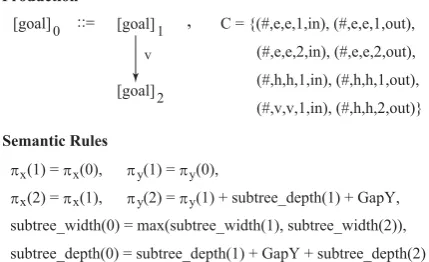
The production and semantic rules shown in Figure10are as formalized for the ‘and’ operation on Prolog goals. Semantic rule πx(2) =πx(1) +subtree width(1) +GapX means that the x-coordinate of node 2 is equal to the x-x-coordinate of node 1 plus the width of the subdiagram derived from node 1 plus the horizontal gap ‘GapX’. Therefore, goals connected by the operator ‘and’ are aligned with a separation of ‘GapX’ in the horizontal direction.
The production and semantic rules shown in Figure11are as formalized for the ‘or’ operation on Prolog goals. Semantic rule πy(2) =πy(1) +subtree depth(1) +GapY means that the y-coordinate of node 2 is equal to the y-y-coordinate of node 1 plus the depth of the subdiagram derived from node 1 plus the horizontal gap ‘GapY’. Therefore, goals connected by the operator ‘or’ are aligned with a separation of ‘GapY’ in the vertical direction.
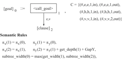
The production and semantic rules shown in Figure12 are formalized for the call of a goal. Semantic ruleπy(2) =πy(1) +depth(1) +GapY means that the y-coordinate of node 2 is equal to the y-coordinate of node 1 plus the depth of the cell corresponding to node 1 plus the vertical gap ‘GapY’. Therefore, a calling goal and the clause heads of the goals called by it are aligned with a separation of ‘GapY’ in the vertical direction.
Figure 13 shows the rules for drawing negated goals. Figure14 shows the production and
[goal]
0 ::= 1 2
[goal] [goal]
C = {(#,e,e,1,in), (#,e,e,2,out), (#,h,h,1,in),
(#,h,h,2,out), (#,v,v,1,in), (#,v,v,1,out)}
Semantic Rules
π (1) = π (0), π (1) = π (0),
π (2) = π (1) + subtree_width(1) + GapX, π (2) = π (1),
subtree_width(0) = subtree_width(1) + GapX + subtree_width(2),
subtree_depth(0) = max(subtree_depth(1), subtree_depth(2))
Production x y x [ x [ x [ , e,h
Figure 10: Rules formalized for ‘and’ operation on Prolog goals
[goal]
0 ::= 1
2
[goal]
[goal]
C = {(#,e,e,1,in), (#,e,e,1,out),
(#,e,e,2,in), (#,e,e,2,out),
(#,h,h,1,in), (#,h,h,1,out),
(#,v,v,1,in), (#,h,h,2,out)}
Semantic Rules
π (1) = π (0), π (1) = π (0),
π (2) = π (1), π (2) = π (1) + subtree_depth(1) + GapY, subtree_width(0) = max(subtree_width(1), subtree_width(2)),
subtree_depth(0) = subtree_depth(1) + GapY + subtree_depth(2) Production
x
y
x x y
y
x y
,
v
Figure 11: Rules formalized for ‘or’ operation on Prolog goals
to built-in predicates such as ‘write’, ‘nl’, and the cut ‘!’.
4
Attribute evaluation of Logichart-AGG
The definitions of an edNCE graph grammar, its leftmost derivation, an attribute graph grammar, and attribute evaluation algorithms are outlined in the appendix.
The productions and semantic rules of the Logichart-AGG are defined so as to guarantee that the simple one-pass evaluator described in Figure16in the appendix will evaluate all attribute instances of every c-derivation tree of the Logichart-AGG.
Theorem 2 The Logichart-AGG is a simple one-pass.
An L-TSD is obtained by removing all edges labeled ‘e’ from a diagram derived by the Logichart-AGG. The semantic rules of the Logichart-AGG guarantee the next theorem.
0 ::=
1
2
[goal]
[clause]
C = {(#,e,e,1,in), (#,e,e,1,out), (#,h,h,1,in), (#,h,h,1,out), (#,v,v,1,in), (#,v,v,2,out)}
Semantic Rules
π (1) = π (0), π (1) = π (0),
π (2) = π (1), π (2) = π (1) + get_depth(1) + GapY, subtree_width(0) = max(get_width(1), subtree_width(2)), subtree_depth(0) = get_depth(1) + GapY + subtree_depth(2)
Production
<call_goal>
x x y y
x x y y
,
e,v
Figure 12: Rules formalized for call of goal
0 ::=
1
[goal]
C = {(#,e,e,1,in), (#,e,e,1,out), (#,h,h,1,in), (#,h,h,1,out),
(#,v,v,1,in), (#,v,v,2,out)}
Semantic Rules
π (1) = π (0), π (1) = π (0),
π (2) = π (1), π (2) = π (1) + get_depth(1) + GapY,
π (3) = π (2) + get_width(2) + GapX, π (3) =π (2),
subtree_width(0) = max(get_width(1), get_width(2) + GapX + subtree(3)),
subtree_depth(0) = get_depth(1) + GapY + max(get_depth(2), subtree(3))
Production
<negation_goals>
<negation_goals>
2
[goal]3
Z x y y
Z x y y
Z x y y
, e,v
e,h
Figure 13: Rules formalized for negation of goals
C3∧C4∧C5∧C6.
The above theorem states that the diagrams derived by the Logichart-AGG are the minimum-area ones under the layout constraint,B1∧B2∧B3∧B4∧B5∧B6.
5
Conclusion
0::=
1 [goal]
C = {(#,e,e,1,in), (#,e,e,1,out),
(#,h,h,1,in), (#,h,h,1,out),
(#,v,v,1,in), (#,v,v,1,out)}
Semantic Rules
π (1) = π (0), π (1) = π (0), subtree_width(0) = get_width(1),
subtree_depth(0) = get_depth(1) Production
<built-in_predicate>
x x y y
,
Figure 14: Rules formalized for built-in predicates
the Logichart-AGG. The diagrams derived by the Logichart-AGG were the minimum-area ones under the specific layout constraint.
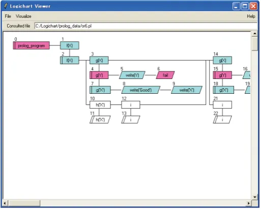
We implemented a Prolog visualization system in complete accordance with the Logichart-AGG in the SICStus prolog [12]. The system inputs a prolog program and a query, parses them (and does not parse a graph grammar), generates an internal representation of the corresponding
Logichart diagram, and displays them with Tcl/Tk. Figure15 shows a snapshot of the Prolog
visualization system.
Bibliography
[1] Eisenstadt M. and Brayshaw M.: A fine-grained account of Prolog execution for teaching and debugging,Instructional Science, Vol.19, No.4, pp.407-436 (1990).
[2] Brayshaw M. and Eisenstadt M.: A practical graphical tracer for Prolog,J. Man-Machine
Studies, 35, pp.597-631 (1991).
[3] Tamir D.E.: A visual debugger for pure Prolog,INFORMATION SCIENCES, Vol.3, No.2,
pp.127-147 (1995).
[4] Adachi Y., Imaki T., Tsuchida K. and Yaku T.: Program visualization by attribute graph
grammars,Proc. CDROM The Fundamental Conference of 15th IFIP WCC’98, (1998).
[5] Adachi Y., Tsuchida K., Imaki T. and Yaku T.: Logichart - Intelligible Program Diagram for Prolog and its Processing System, Electronic Notes in Theoretical Computer Science, Volume 30, Issue 4, Elsevier Science (2000).
[6] G¨ottler H.: Attribute Graph Grammar for Graphics, Lecture Notes in Computer Science,
Vol.153, pp.130-142 (1982).
[7] Nishino T.:, Attribute graph grammars with applications to Hichart editors,Adv. Software Sci. & Tech., 1, pp.426-433 (1989).
[8] Engelfriet J. and Rozenberg G.: Node Replacement Graph Grammar, in Handbook of
Graph Grammars and Computing by Graph Transformation(Rozenberg, G., eds), World Scientific, pp.1-94 (1997).
[9] Goto T., Kirishima T., Motousu N., Tsuchida K. and Yaku T.: A visual software
devel-opment environment based on graph grammars, IASTED Conf. on Software Engineering,
pp.620-625 (2004).
[10] Crescenzi P., Battista Di and Piperno A.: A note on optimal area algorithms for upward
drawings of binary trees,Computational Geometry: Theory and Applications, 2:187-200
(1992).
[11] Eades P., Lin T. and Lin X.: Minimum size h-v drawings, Advanced Visual Interfaces,
pp.386-394, World Scientific (1992).
[12] “Sicstus syntax”, http://www.sics.se/ps/sicstus.html.
[13] Kaplan S.M. and Goering S.K.: Priority Controlled Incremental Attribute Evaluation in
Attribute Graph Grammars,TAPSOFT, Vol.1, pp.306-336 (1989).
[14] Maneth S. and Vogler H.: Attribute Context-Free Hypergraph Grammars, J. Automata,
Appendix
We outline an edNCE grammar that generates ordered graphs, leftmost derivations, and c-derivation trees by referring to [8].
Attribute graph grammars were developed in the 1980s [6]. Some attribute evaluation algo-rithms for attribute graph grammars have been published (e.g., [13, 14]). Here, we explain an attribute graph grammar whose underlying grammar is the edNCE grammar that generates or-dered graphs. We then explain an attribute evaluation algorithm on the basis of the node order of the right-hand side graphs of the edNCE grammar’s productions and their c-derivation trees.
A
Graph grammar and derivation
A.1 edNCE grammar
LetΣbe an alphabet of nodes andΓbe an alphabet of edges. AgraphoverΣandΓis a 3-tuple
H= (V,E,λ), whereVis the finite nonempty set of nodes,E⊆ {(v,γ,w)|v,w∈V,v6=w,γ∈Γ} is the set of edges, andλ :V→Σis the node labeling function. The components of a graph,H, are denoted byVH,EH, andλH. Two graphsH andKareisomorphicif there is a bijection f :
VH→VKsuch thatEK={(f(v),γ,f(w))|(v,γ,w)∈EH}and, for allv∈VH,λK(f(v)) =λH(v). The set of all graphs overΣandΓis denoted asGRΣ,Γ.
Definition 6 AnedNCE grammaris a tupleG= (Σ,∆,Γ,Ω,P,S), where
(1) Σis the alphabet of node labels.
(2) ∆is the alphabet of terminal node labels. (3) Γis the alphabet of edge labels.
(4) Ωis the alphabet of final edge labels.
(5) Pis the finite set of productions. A production has the form ‘X →(D,C)’, where
(5.1) X∈Σ−∆andD∈GRΣ,Γ.
(5.2) C⊆Σ×Γ×Γ×VD× {in, out} is the connection relation of p and each element
(σ,β,γ,x,d) (σ∈Σ,β,γ∈Γ,x∈VD,d∈ {in, out})ofCis a connection instruction ofp.
(6) S∈Σ−∆is the initial nonterminal node label. Theinitial graph,Hs, is a graph that consists of a single node labeledSand has no edge.
Two productions p1:X1→(D1,C1)andp2:X2→(D2,C2)are called isomorphic ifX1=X2
and there is an isomorphism f fromD1 toD2andC2={(σ,β,γ, f(x),d)|(σ,β,γ,x,d) ∈
C1}. By copy(p), we denote the set of all productions that are isomorphic to a production, p, in
P. An element of copy(p)is called aproduction copyofp. copy(P) = [
p∈P
The process of graph rewriting in an edNCE graph grammar is defined as follows. Let a given graph (host graph) beHand letvbe a nonterminal node ofH. Let nodevbe labeledX, and let
p0:X→(D0,C0)be a production copy of somep∈Psuch thatD0 andHare mutually disjoint.
(1) Remove nodevand all edges that are incident withvfromH. Let the resulting graph (rest graph) beH−.
(2) PutD0(daughter graph) inH−.
(3) Establish new edges between certain nodes ofD0and certain nodes ofH− in a way spec-ified by the connection instructions inC0. This is called the embedding ofD0inH−. Let the resulting graph beH0.
The meaning of an instruction, (σ,β,γ,x, in)∈C0, is as follows: if there is an edge with labelβ from a node,w∈VH− {v}, with labelσ to nodev, then the embedding process should
establish an edge with labelγ from nodewto nodex∈VH0. Also, this is similarly the case for (σ,β,γ,x,out)instead of(σ,β,γ,x,in), where ‘in’ refers to the incoming edges ofvand ‘out’ to the outgoing edges ofv.
LetHandH0be graphs inGRΣ,Γ. IfHis transformed intoH0by the application of a production
copy, p0, as described above, then we writeH⇒v,p0H0and call it aderivation step. A sequence of derivation stepsH0⇒v1,p0
1 H1 ⇒v2,p02 · · · ⇒vn,p0n Hnis called a derivation. A derivation,H0 ⇒v
1,p01
H1⇒v
2,p02
· · · ⇒v
n,p0nHn,n≥0, iscreativeif the graphs,H0andD
0
i, 1≤i≤n, are mutually disjoint, where rhs(p0i) = (D0i,C0i). We will restrict ourselves to creative derivations. We write
H⇒∗H0if there is a creative derivation as above, withH0=HandHn=H0. Asentential formof
Gis a graph,H, such thatHS⇒∗Hfor some initial graphHS. A set of sentential forms is denoted byS(G). Thegraph language generated by GisL(G) ={[H]|H ∈GR∆,ΩandHS⇒∗Hfor some initial graphHS}. For a graph,H, the set of all graphs isomorphic toHis denoted as[H].
A.2 Leftmost derivation
The leftmost derivation is defined as follows. Let a given ordered graph (host graph) beH and letvbe the first nonterminal node within the node order ofH. Let nodevbe labeledX, and let
p0:X→(D0,C0)be a production copy of somep∈Psuch thatD0 andHare mutually disjoint.
(1) Remove nodevand all edges that are incident withvfromH. Let the resulting graph (rest graph) beH−.
(2) PutD0(daughter graph) inH−.
(3) Establish new edges between certain nodes of D0 and certain nodes of H− in the way
specified by the connection instructions inC0. Let the resulting graph beH0.
(4) If the nodes ofH are ordered as(v1,· · ·,vh)with v=vi, and those ofD0 are ordered as
(w1,· · ·,wd), then the order,H0, isv1,· · ·,v(i−1),w1,· · ·,wd,v(i+1),· · ·,vh.
copy, p0, as described above, then we writeH⇒p0H0 and call it a leftmost derivation step. A sequence of leftmost derivation steps H0 ⇒v
1,p01
H1 ⇒v
2,p02
· · · ⇒v
n,p0n Hn is called a leftmost derivation.
We writeH⇒∗lmH0if there is a leftmost derivation fromHtoH0. Thegraph language leftmost generated by GisLlm(G) ={[H]|H∈GR∆,ΩandHS⇒∗lmHfor some initial graphHS}, where the abstract graph,[H], no longer involves an order.
A.3 Derivation tree
Derivation trees are rooted, ordered trees. Each vertex of a tree has directed edges to each of its
kchildren,k≥0, and the order of the children is indicated by labeling the edges as 1,· · ·,k.
Definition 7([8]) LetG= (Σ,∆,Γ,Ω,P,S) be an edNCE grammar. Ac-labeled derivation treeofGis a rooted, ordered treetwhose vertices are labeled by production copies incopy(P), such that
(1) the right-hand sides of all the production copies that label the vertices oft are mutually disjoint, and do not contain the root oftas a node, and
(2) if vertexvofthas labelX→(D,C), then the children ofvare the nonterminal nodes ofD, and their order intis the same as their order inD; moreover, for each childw, the left-hand side of the label ofwintequals its label inD.
If the root of a derivation tree,t, is labeled with productionX→(D,C), then we also say that
tis a derivation treefor X (note that not necessarilyX=S).
B
AGG and attribute evaluation
B.1 Definition of AGG
An AGG in this work is defined by referring to [7].
Definition 8 Anattribute graph grammar(AGG) is a tupleAG=<G,A,F>, where
(1) G= (Σ,∆,Γ,Ω,P,S)is an edNCE grammar that generates order graphs and we call it an
underlying graph grammarofAG.
(2) Each node labelX ∈ΣofGhas two disjoint finite setsInh(X)andSyn(X) ofinherited andsynthesized attributes, respectively. We denote the set of all attributes of nonterminal node symbolX byA(X) =Inh(X)∪Syn(X).A= [
X∈Σ
A(X)is called theset of attributesof
G. We assume thatInh(S) =φ, and that for eachX∈∆Syn(X) =φ. An attribute ofX is
denoted bya(X), and the set of possible values ofais denoted byV(a).
(3) Associated with each production p:X0 →(D,C) is a set Fp of semantic rules, which define all the attributes inSyn(X0)∪Inh(X1)∪ · · · ∪Inh(Xn)whereVD={v1,· · ·,vn}and
a(Xk):= f(a1(Xi1), . . . ,am(Xim)),where f is a mapping, V(a1(Xi1))×. . .×V(am(Xim))
intoV(a(Xk)). In this situation, we say thata(Xk)depends ona1(Xi1),· · ·,am(Xim)in p.
The set,F= [
n∈P
Fp, is called theset of semantic rulesofAG.
B.2 Attribute evaluation algorithm
The graph nodes generated by AGGs have no natural linear ordering. Therefore, to evaluate attributes properly, we need to first decide the order in which the vertices of the c-derivation trees of the AGG are traversed. To do this, we use an edNCE grammar that generates ordered graphs as the underlying grammar of the AGG. The vertices of c-derivation trees are then traversed in the node order of the right-hand side graphs of the edNCE grammar’s productions.
An AGGGis asimple one-passif the simple-pass evaluator given in Figure16evaluates all attribute instances of every c-labeled derivation tree for theS ofG. The simple-pass evaluator traverses the vertices of a c-derivation treetin depth-first and then from left to right.
procedureEVALUATE(v0);vertexv0;
{Let the label of vertexv0beX→(D,C)and let the nodes
ofDbe ordered asv1,v2,· · ·,vn.}
begin
compute all inherited attributes ofX; fori:=1tondo
begin
ifviis a nonterminal nodethenEVALUATE(vi);
elsecompute all attributes ofλD(vi);
end
compute all synthesized attributes ofX; end
Simple one-pass begin
EVALUATE(root); end
![Figure 9: Rules used to rewrite initial node ‘[ prolog program ]’](https://thumb-us.123doks.com/thumbv2/123dok_us/7819869.2087403/9.595.181.416.358.465/figure-rules-used-rewrite-initial-node-prolog-program.webp)