Available online throug
ISSN 2229 – 5046
TRANSIENT CONVECTIVE HEAT AND MASS TRANSFER FLOW OF A CHEMICALLT
REACTING VISCOUS FLUID PAST A STRETCHING SHEET WITH HALL CURRENTS,
RADIATION ABSORPTION, DISSIPATION, NON-UNIFORM HEAT SOURCES
B. ALIVENE
#1, Dr. M. SREEVANI
2#1
Research Scholar, Department of Mathematics,
Rayalaseema University, Kurnool-518007(AP), India.
2
Department of Mathematics, S.K.U. College of Engineering &Technology,
Sri krishnadevaraya University, Anantapuramu – 515003 (AP), India.
(Received On: 05-11-17; Revised & Accepted On: 18-11-17)
ABSTRACT
I
n this paper, we study the unsteady convective heat and mass transfer flow of a viscous electrically conducting fluid through a porous medium past a stretching sheet with Hall effects, dissipation, chemical reaction and radiation absorption in the presence of non-uniform heat source.. The equations governing the flow of heat and mass transfer have been solved numerically. The velocity, temperature and concentration have been analysed for different values of G, M, m, N, γ, A1, B1, Sc, Ec and Q1. The rate of heat and mass transfer on the plate has been evaluated numericallyfor different variations.
Keywords: Radiation Absorbtion, Hall Currents, Non-Uniform Heat Sources, Dissipation,Chemical Reaction.
INTRODUCTION
Mixed convection boundary layer flow of a binary mixture of fluids with heat and mass transfer past a continuous moving surface has attracted considerable attention in the past several decades, due to its many important engineering and industrial applications (9, 13). In nature such flows are encountered in the oceans, lakes, solar ponds, and the atmosphere. They are also responsible for the geophysics of planets.
The effect of chemical reaction on free convective flow and mass transfer of a viscous, incompressible and electrically conducting fluid over a stretching sheet was investigated by Afify [2] in the presence of a transverse magnetic field. In all these investigations the electrical conductivity of the fluid was assumed to be uniform. However, in an ionized fluid where the density is low and/or magnetic field is very strong, the conductivity normal to the magnetic field is reduced due to the spiralling of electrons and ions about the magnetic lines of force before collisions take place and a current induced in a direction normal to both the electric and magnetic fields. This phenomenon available in the literature is known as Hall Effect. Thus the study of MHD viscous flows, heat and mass transfer with Hall currents has important bearing in the engineering applications.
Hall effect on MHD boundary layer flow over a continues semi-infinite flat plate moving with a uniform velocity in its own plane in an incompressible viscous and electrically conducting fluid in the presence of a uniform transverse magnetic field were investigated by Watanabe and Pop [18]. Abdullah [1] have investigated free convective flows past a semi-infinite vertical plate with mass transfer. The effect of Hall current on the study MHD flow of an electrically conducting, incompressible Burger’s fluid between two parallel electrically insulating infinite plane was studied by Rana et al. [12].
Corresponding Author: B. Alivene
#1,
#1
Research Scholar, Department of Mathematics,
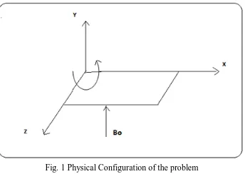
Fig. 1 Physical Configuration of the problem
In all the above studies the physical situation is related to the process of uniform stretching sheet. For the development of more physically realistic characterization of the flow configuration it is very useful to introduce unsteadiness into the flow, heat and mass transfer problems. The working fluid heat generation or absorption effects are very crucial in monitoring the heat transfer in the regions, heat removal from nuclear fuel debris, underground disposal of radioactive waste material, storage of food stuffs, exothermic chemical reactions and dissociating fluids in packed-bed reactors. This heat source can occurs in the form of a coil or battery. Very few studies have been found in literature on unsteady boundary flows over a stretching sheet by taking heat generation/absorption into the account Several Authors (3, 4, 5, 7, 10, 11, 13, 14, 15, 16) have studied unsteady convective heat and mass transfer in different configurations under varied conditions.
FORMULATION OF THE PROBLEM:
We consider the unsteady flow of an incompressible, viscous, electrically conducting fluid through a porous medium past a permeable vertical stretching sheet coinciding with the plane y=0 and the flow is confined to the region y>0.A schematic representation of the physical model is exhibited in fig.1.We choose the frame of reference (x,y,z) such that the x-axis is along the direction of motion of the surface,the y-axis is normal to the surface and z-axis transverse to the x-y-plane.An external constant magnetic field H0 is applied in the positive y-direction. The surface of the sheet is assumed to have a variable temperature Tw(x), while the ambient fluid has a uniform temperature
T
∞, whereTw(x)>
T
∞ corresponds to a heated plate and Tw(x)<T
∞,corresponds to a cooling plate..The effects of Hall currents, viscous dissipation, radiation absorption and the first order chemical reaction are considered. Using boundary layer approximation, Boussinesq’s approximation and taking Hall current into account the governing equations are0
=
∂
∂
+
∂
∂
y
v
x
u
(1)
2 2
2 0 2
(
)
(
) ( )
(
)
(1
)
u
u
u
u
u
v
g T
T
g C
C
u
t
x
z
y
k
B
u
mw
m
µ
ν
β
β
σ
ρ
∗
∞ ∞
∂
+
∂
+
∂
=
∂
+
−
+
−
−
−
∂
∂
∂
∂
−
+
+
(2)
2 2
0
2
( )
2(
)
(1
)
B
w
w
w
w
u
v
v
mu
w
t
z
z
y
k
m
σ
µ
ν
ρ
∂
+
∂
+
∂
=
∂
−
+
−
∂
∂
∂
∂
+
(3)2
2 '
1 2
(
)
(
)
(
)
p f
T
T
T
T
u
C
u
v
k
q
Q C C
t
x
y
y
y
ρ
µ
∞∂
+
∂
+
∂
=
∂
+
′′′
+
∂
+
−
∂
∂
∂
∂
∂
(4)2 0 2
(
C
u
C
v
C
)
D
BC
k C C
(
)
t
x
y
y
∞∂
+
∂
+
∂
=
∂
−
−
∂
∂
∂
∂
(5)The energy equation with thermal radiation and Non-Uniform heat source reduces to
(
) ( )
(
)
2 2
3 2
2 '
1 2
1
1
16
(
)
(
)
3
p f w
R
T
T
T
C
u
w
k
A T
T
f
B T
T
x
z
y
T
u
T
Q C
C
y
y
ρ
η
σ
µ
β
∞ ∞
∗ ∞ ∞
∂
∂
∂
+
=
+
−
′
+
−
+
∂
∂
∂
∂
∂
+
+
−
+
∂
∂
(6)
The boundary conditions for this problem can be written as
( , ),
( , ),
0,
(
( , 0)),
(
( , 0)),
0
w w
f T w B c w
u
U
x t v
V x t w
T
C
k
h T
T x
D
h C C
x
at y
y
y
=
=
=
∂
∂
−
=
−
−
=
−
=
∂
∂
(7)
∞
→
=
=
=
=
w
T
T
∞C
C
∞as
y
1/ 2
( , )
(
)
(0)
w
Uw
v
x t
f
x
ν
= −
represents the mass transfer at the surface with Vw>0 for injection and Vw>0 forsuction. The flow is caused by the stretching of the sheet which moves in ite own plane with the surface velocity
( , )
,
(1
)
w
ax
U
x t
ct
=
−
where a (stretching rate) and c are the positive constants having dimension time -1(with t<1,
c≥0).It is noted that the stretching rate
(1
)
a
ct
−
increases with time ,since a>0. The surface temperature and concentration of the sheet varies with the distance x from the slot and time t in the form so that surface temperature2 3/ 2
( , )
2 (1
)
w
ax
T x t
T
ct
ν
∞
=
+
−
and surface concentration2 3/ 2
( , )
2 (1
)
w
ax
C x t
C
ct
ν
∞
=
+
−
where a≥0 .The particular form ofU
w( , ),
x t T x t a n d
w( , )
C
w( , )
x t
has been chosen in order to derive a similarity transformation whichtransforms the governing partial differential equations (2)-(5) into a set of highly nonlinear ordinary differential equations.
The stream function ѱ(x,t) is defined as:
( ),
( )
(1
)
(1
)
ax
a
u
f
v
f
y
ct
x
ct
ψ
η
ψ
ν
η
∂
′
∂
=
=
= −
=
∂
−
∂
−
(9)On introducing the similarity variables (Dulal Pal [5]):
(1
)
a
y
ct
η
=
−
(10)1/ 2
( , , )
(
)
( ),
(
) ( )
1
1
a
ax
x y t
xf
w
g
ct
ct
ν
ψ
=
η
=
η
−
−
(11)2 3/ 2
( , . )
( ), ( )
2 (1
)
wT
T
ax
T x t t
T
ct
θ η θ η
T
T
ν
∞∞
∞
−
=
+
=
−
−
(12)2 3/ 2
( , . )
( ), ( )
2 (1
)
wC
C
ax
C x t t
C
ct
φ η φ η
C
C
ν
∞∞
∞
−
=
+
=
−
−
(13)2 2 1
(1
)
o
B
=
B
−
ct
− (14)Non dimensional Parameters.
Using (Equations (10) - (14) into equations (2),(3),(5) and (7) we get
2 1
2 2
(
1.5
)
(
)
(
)
0
1
f
f f
f
S f
f
G
N
D f
M
f
mg
m
θ
ϕ
−′′′
+
′′
−
′
−
′
+
′′
+
+
−
′
−
′
−
+
=
+
(15) 1 2 2(
1.5
)
(
)
0
1
g
fg
f g
S g
g
D g
M
mf
g
m
−′′
+
′
−
′
−
′
+
′′
−
+
′
+
−
=
+
(16)(
)
1 24
(1
)
(
2
0.5 (3
)
3
(
)
1
0
r
Nr
P
f
f
S
P A f
B
Ec f
Q
θ
θ
θ
θ ηθ
θ
φ
∗ ∗′′
′
′
′
′
+
+
−
−
+
+
+
+
′′
+
+
=
(17)(
2
0.5 (3
)
0
Sc f
f
S
Sc
ϕ
′′
+
φ
′
−
′
φ
−
φ ηφ
+
′
−
γ φ
=
(18) Where S=c/a, 2 0B
M
a
σ
ρ
=
,D
1ak
ν
−
=
,
(
w 2)
w w
g T
T
G
U v
β
−
∞=
(
)
(
)
w wC
C
N
T
T
β
β
∗ ∞ ∞−
=
−
,Pr
2
(
)
w P wU
Ec
C T
T
∞=
−
, ' 1 1 2 wQ
Q
v
ν
=
, BSc
D
ν
=
,m
=
ω τ
e e ,2 o w
k
v
ν
γ
=
,3
4
R fT
Nr
k
σ
β
∗ ∞=
are the non-dimensional parameters defined in the nomenclature of the thesis.
The transformed boundary conditions (7) & (8) reduce to
(0) 1,
(0)
,
(0)
0,
(0)
c(1
(0)), (0)
i(1
(0))
f
f
fw
g
B
B
θ
θ
φ
φ
′
=
=
=
′
= −
−
′
= −
−
(19)( )
0, ( )
0, ( )
0, (0
)0
f
′ ∞ →
g
∞ →
θ
∞ →
φ
→
(20)SKIN FRICTION, NUSSELT NUMBER and SHERWOOD NUMBER
The physical quantities of engineering interest in this problem are the skin friction coefficient Cf, the Local Nusselt number Nux, the Local Sherwood number Shx which are expressede as
1
1
(0),
(0),
2
C
fR
ex=
f
′′
2
C
fzR
ez=
g
′
Nux
/
R
ex= −
θ
′
(0) ,
Shx
/
R
ex= −
φ
′
(0)
Where p
k
C
µ
ρ
=
is the dynamic viscosity of the fluid and Rex is the Reynolds number.METHOD OF SOLUTION
The non-linear equations (15)-(18) have been solved by employing Galerkin finite element technique with quadratic polynomials.The variational form associated with the equations (17)-(20) over a typical two nodded line at element(
η
e,
η
e+1)
is given by∫
+1 1(
′
−
)
=
0
e e
d
h
f
w
η ηη
(21)1 2
2
12
(
(
1.5 )
(
)
2(
))
0
1
e
e
M
w
h
fh
h
S h
h
G
N
h
mg d
m
ηη
θ
ϕ
η
+
′′
+
′
−
−
+
′
+
+
−
+
=
+
∫
(22)1 2 2
3
(
(
1.5
) (
2)
2)
0
1
1
e
e
M
mM
w g
fg
S g
g
h
g
h d
m
m
η ηη
+′′
+
′
−
′
+
′′
− +
+
=
+
+
∫
(23)(
)
( )
1 2
2
4 1 2
4
((1 ) ( 2 0.5 (3 ) 1 1 ) 0
3 1
e
e
r
r r
N M Ec
w P f f S Q P A h B h d
m
η
η
θ θ θ θ ηθ φ θ η
+ ′′ ′ ′ ′ + + − − + + + + + = +
∫
(24) 15
(
(
) 0.5 (3
)
)
0
e
e
w
Sc
f
S
ScSo
d
η
η
φ
φ
γφ
φ ηφ
θ
η
+
′′
+
′
−
−
+
′
+
′′
=
∫
(25)where w1, w2, w3, w4, w5 are arbitrary test functions and may be regarded as the variations in f, h, g, θ and
φ
respectively. The finite element method may be obtained from (21)-(25) by substituting finite element approximations of the form∑
==
3 1 k k kf
f
ψ
,=
∑
=3 1 k k k
h
h
ψ
,∑
=
=
3 1 k k kg
g
ψ
,∑
=
=
3 1 k k kψ
θ
θ
,∑
=
=
3 1 k k kψ
φ
φ
(26)By taking w1=w2=w3=w4=w5= j
(
i
,
j
=
1
,
2
,
3
)
iψ
Using (26) in equations (21) - (25) and evaluating the integrals we get local stiffness matrix of order 3x3 in the form.
)
(
)
(
)
(
1
)
(
)
2
1
)(
(
2 1, 2,2 , k j k j k i k i k i k i k j
i
g
Q
Q
m
M
NC
G
u
R
f
=
+
+
+
+
−
−
θ
(27))
(
)
(
)
(
1
)
)(
2
1
(
)
(
2 1, 2,2 , k j k j k i k i k j
i
u
R
R
m
mM
f
R
g
=
+
+
−
+
( )( )
( )
(
)
(
)
)
(
)
)(
1
)(
(
, 1, 2,* 1 2
1 *
1 2 ,
k j k
j k
j i k
i k i k
i k
i k
j
i
N
P
B
P
u
Q
N
m
P
A
m
S
S
e
+
α
+
θ
−
−
φ
−
=
+
(29)
, , 1, 2,
(
l
i jk)(
φ
ik)
−
Sc u
(
ik)(
φ
ik)
+
ScSo n
(
i jk)(
θ
ik)
=
(
T
kj)
+
(
T
kj)
(30)where
(
,k)
j i
f
,(
k,)
j i
g
,(
k,)
j i
θ
,(
k,)
j i
φ
,(
k,)
j i
e
,(
k,)
j i
l
,( )
m
ik,j ,(
k,)
i j
n
are 3x3 matrices and)
.(
)
(
),
(
),
(
),
(
),
(
),
(
),
(
1, 2, 1, 1, 1, 1, 1, 1,k jj k
jj k
jj k
jj k
jj k
jj k
jj k
jj
Q
R
R
S
S
T
and
T
Q
are 3x1 column matrices and such stiffnessmatrices (29)-(30) in terms of local nodes in each element are assembled using inter element continuity and equilibrium conditions to obtain the coupled global matrices in terms of the global node values of h, f, g, θ and
φ
.The ultimate coupled global matrices are solved to determine the unknown global values of velocity, temperature and concentration in the fluid region. In solving these matrices an iteration procedure has been adopted. The iteration process is repeated until the absolute values of the difference between two consecutive values differ by a preassigned approximation.COMPARSON
Table-1: Comparison of Nu (0) for M=m=G=N=Ec=Q1=Sc=fw=γ=0, A1=B1=0
Pr Chen(4a) Grubka and Bobba (8) Aziz(6) Sarojamma et al (14) Present results
0.01 0.02942 0.0294 0.02948 0.02949 0.02952
0.72 1.08853 1.0885 1.08855 1.08857 1.08859
1.0 1.33334 1.3333 1.33333 1.33335 1.33336
3.0 2.50972 2.5097 2.50972 2.50974 2.50976
7.0 3.97150 3.97151 3.97152 3.97155
10.0 4.79686 4.7969 4.79687 4.79688 4.79689
100.0 15.7118 15.712 15.7120 15.7122 15.7123
RESULTS AND DISCUSSION
In order to validate the accuracy of the numerical scheme employed we have compared the local temperature gradient of the present analysis with those of Chen (4a). Grubka and Bobba(8), Aziz(6) and Sarojamma et al. (14) for different values of Prandtl number in absence of magnetic field,thermal and solutal buoyancy,radiation absorption,viscous dissipation and suction for steady flow M=A=Gr=N=γ=Q1=Ec=Sc=fw=A1=B1=0 and presented in table.1 and are found to be in good agreement.
Figs.2 - 5 represents the velocity components, temperature and concentration wit Hall parameter (m). As mentioned above the Lorentz force has a retarding effect on the primary velocity, this retardation is enhanced with increase in the Hall parameter and hence the primary velocity is enhanced and consequently the momentum boundary layers become thinner. The secondary velocity increases as the Hall parameter increases. The effect of Hall parameter on temperature and concentration is to diminish them as a consequence of reducing the thermal and solutal boundary layers. Skin friction component τx, Nusselt number Nu, Sherwood number sh decreases and skin friction component τz increases with G at η=0.
Figs.6-9 represent the velocity components, temperature and mass concentration with heat generating/absorption source. An increase in the space dependent/temperature dependent degenerating source enhances the primary velocity owing to the generation of energy in the boundary layer while in the case of heat absorption source, the primary velocity reduces in the boundary layer owing to the absorption in the boundary layer. The secondary velocity, temperature and mass concentration reduce with strength of heat degenerating /absorption source.
The effect of chemical reaction parameter (γ) on the velocity, temperature and concentration can be seen from figs.10-13. It can be observed from the figures the velocity components increases in both degenerating and generating chemical reaction cases.The temperature increases and the concentration reduces in the degenerating chemical reaction case while a reversed effect is noticed in temperature and concentration in generating chemical reaction case. This is due to the fact that the thickness of the momentum boundary layer increases with increase in the chemical reaction parameter
γ.An increase in γ>0, reduces the thermal boundary layer and reduces the solutal boundary layer while a reversed effect is noticed in the thickness of the thermal and solutal boundary layer thickness.Skin friction components τx,τy increases where γ>0 and Skin friction components τx decreases ,τy increases when γ<0. Nusselt number Nu increases whenγ>0 and Nusselt number Nu decreases whenγ<0. Sherwood number decreases when γ>0 and Sherwood number increases when γ<0 with γ at η=0.
thermal and solutal boundary layers and for higher Q1≥2, they reduce. Skin friction components τx,τy and Nusselt number, Sherwood number decreases with Q1 atη=0.
Fig.2: Variation of f′ with m
G = 2, M=0.5, D-1=0.2,N=1,A1,B1=0.1, Sc=1.3,
γ=0.5, Q1=0.5, Ec=0.01, fw=0.2, s=0.5, Pr=0.71
0 0.2 0.4 0.6 0.8 1
0 1 2 3 4 5 6
η
f '
m = 0.5,1,1.5,2
Fig.3: Variation of g with m
G = 2, M=0.5, D-1=0.2,N=1,A1,B1=0.1, Sc=1.3,
γ=0.5, Q1=0.5, Ec=0.01, fw=0.2, s=0.5, Pr=0.71
0 0.02 0.04 0.06 0.08 0.1 0.12
0 1 2 3 4 5 6
η g
m = 0.5,1,1.5,2
Fig.4: Variation of θ with m
G = 2, M=0.5, D-1=0.2,N=1,A1,B1=0.1, Sc=1.3,
γ=0.5, Q1=0.5, Ec=0.01, fw=0.2, s=0.5, Pr=0.71
0 0.2 0.4 0.6 0.8 1
0 1 2 3 4 5 6
η θ
m = 0.5,1,1.5,2
Fig.5: Variation of C with m
G = 2, M=0.5, D-1=0.2,N=1,A1,B1=0.1, Sc=1.3,
γ=0.5, Q1=0.5, Ec=0.01, fw=0.2, s=0.5, Pr=0.71
0 0.2 0.4 0.6 0.8 1
0 1 2 3 4 5 6
η C
m = 2, 0.5,1,1.5
Fig.6: Variation of f′ with A1,B1
G = 2, M=0.5,m=0.5,D-1=0.2,N=1, Sc=1.3,
γ=0.5, Q1=0.5, Ec=0.01, fw=0.2, s=0.5, Pr=0.71 0
0.2 0.4 0.6 0.8 1
0 1 2 3 4 5 6
η
f '
A1 = 0.1,0.3 B1 = 0.1,0.3
A1 = -0.1,-0.3 B1 = -0.1,-0.3
Fig.7: Variation of g with A1,B1
G = 2, M=0.5,m=0.5,D-1=0.2,N=1, Sc=1.3,
γ=0.5, Q1=0.5, Ec=0.01, fw=0.2, s=0.5, Pr=0.71
0 0.02 0.04 0.06 0.08 0.1
0 1 2 3 4 5 6
η g
Fig.8 : Variation of θ with A1,B1
G = 2, M=0.5,m=0.5,D-1=0.2,N=1, Sc=1.3,
γ=0.5, Q1=0.5, Ec=0.01, fw=0.2, s=0.5, Pr=0.71
0 0.2 0.4 0.6 0.8 1
0 1 2 3 4 5 6
η θ
A1 = 0.1,0.3,-0.1,-0.3 B1 = 0.1,0.3,-0.1,-0.3
Fig.9 : Variation of C with A1,B1
G = 2, M=0.5,m=0.5,D-1=0.2,N=1, Sc=1.3,
γ=0.5, Q1=0.5, Ec=0.01, fw=0.2, s=0.5, Pr=0.71
0 0.2 0.4 0.6 0.8 1
0 1 2 3 4 5 6
η C
A1 = 0.1,0.3,-0.1,-0.3 B1 = 0.1,0.3,-0.1,-0.3
Fig.10: Variation of f′ with γ
G = 2, M=0.5,m=0.5,D-1=0.2,N=1,A1,B1=0.1,
Sc=1.3, Q1=0.5, Ec=0.01, fw=0.2, s=0.5, Pr=0.71 0
0.2 0.4 0.6 0.8 1
0 1 2 3 4 5 6
η
f '
γ = 0.5,1.5,-0.5,-1.5
Fig.11: Variation of g with γ
G = 2, M=0.5,m=0.5,D-1=0.2,N=1,A1,B1=0.1,
Sc=1.3, Q1=0.5, Ec=0.01, fw=0.2, s=0.5, Pr=0.71
0 0.02 0.04 0.06 0.08 0.1 0.12
0 1 2 3 4 5 6
η g
γ = 0.5,1.5,-0.5,-1.5
Fig.12: Variation of θ with γ
G = 2, M=0.5,m=0.5,D-1=0.2,N=1,A1,B1=0.1,
Sc=1.3, Q1=0.5, Ec=0.01, fw=0.2, s=0.5, Pr=0.71
0 0.2 0.4 0.6 0.8 1
0 1 2 3 4 5 6
η θ
γ = -0.5,-1.5
γ = 0.5,1.5
Fig.13: Variation of C with γ
G = 2, M=0.5,m=0.5,D-1=0.2,N=1,A1,B1=0.1, Sc=1.3,
Q1=0.5, Ec=0.01, fw=0.2, s=0.5, Pr=0.71
0 0.2 0.4 0.6 0.8 1
0 1 2 3 4 5 6
η C
γ = -0.5,-1.5
Fig.14: Variation of f′ with Q1
G = 2, M=0.5,m=0.5,D-1=0.2,N=1,A 1,B1=0.1,
Sc=1.3, γ=0.5, Ec=0.01, fw=0.2, s=0.5, Pr=0.71 0
0.2 0.4 0.6 0.8 1
0 1 2 3 4 5 6
η
f '
Q1 = 2.5,0.5,1.5,2
Fig.15: Variation of g with Q1
G = 2, M=0.5,m=0.5,D-1=0.2,N=1,A 1,B1=0.1,
Sc=1.3, γ=0.5, Ec=0.01, fw=0.2, s=0.5, Pr=0.71
0 0.02 0.04 0.06 0.08 0.1 0.12
0 1 2 3 4 5 6
η g
Q1 =0.5,1.5 Q1 = 2,2.5
Fig.16: Variation of θ with Q1
G = 2, M=0.5,m=0.5,D-1=0.2,N=1,A 1,B1=0.1,
Sc=1.3, γ=0.5, Ec=0.01, fw=0.2, s=0.5, Pr=0.71
0 0.2 0.4 0.6 0.8 1
0 1 2 3 4 5 6
η θ
Q1 = 2.5,0.5,1.5,2
Fig.17: Variation of C with Q1
G = 2, M=0.5,m=0.5,D-1=0.2,N=1,A 1,B1=0.1,
Sc=1.3, γ=0.5, Ec=0.01, fw=0.2, s=0.5, Pr=0.71
0 0.2 0.4 0.6 0.8 1
0 1 2 3 4 5 6
η C
Q1 = 2.5,0.5
Q1 = 1.5,2
Table-2: Shear stress, Nusselt number and Sherwood number at η=0
Parameter τx(0) τz(0) Nu(0) Sh(0)
m 0.5 1.0 1.5 2.0
-1.96189 -1.91951 -1.83424 -1.76846
0.031343 0.0359585 0.0368759 0.037507
1.31222 1.29162 1.28803 1.27716
0.0269095 0.0183319 0.0190375 0.0208528
γ 0.5
1.5 -0.5 -1.5
-1.96189 2.01317 -1.75817 -0.70903
0.031343 0.0315259 0.0309097 0.0313241
1.31222 1.31843 1.25728 0.910019
0.0269095 0.00374916 0.192836 0.378216
Ec 0.01 0.03 0.05 0.07
-1.96189 -1.85018 -1.43724 -1.37129
0.031343 0.0308547 0.0288431 0.0258577
1.31222 1.27422 1.16736 1.11541
0.0269095 0.0241738 0.0155667 0.0128883
Q1 0.5
1.0 1.5 2.0
-1.96189 -1.82489 -1.82422 -1.76302
0.031343 0.030767 0.030513 0.028182
1.31222 1.30166 1.29463 1.25653
0.0269095 0.0255907 0.0264386 0.0226858
S 0.1 0.3 0.5 0.7
-1.96189 -1.25068 -0.562785 -0.466763
-1.96189 -1.25068 -0.562785 -0.466763
1.31222 1.34083 1.3638 1.44024
CONCLUSIONS
A mathematical analysis has been made to investigate the effect of chemical reaction radiation absorption on convective heat and mass transfer flow of a viscous, electrically conducting fluid past a porous stretching surface. The coupled equations governing the flow, heat and mass transfer have been solved by employing Finite element method. The effect of various governing parameters on the velocity, temperature and concentrations are the skin friction, the rate of heat and mass transfer on the wall η=0 are evaluated numerically for different variations. From the graphical representations we find that the velocity components enhances in both the degenerating/absorption chemical reaction cases. The temperature, concentration reduces in the degenerating chemical reaction case while a reversed effect is noticed in generating case. Higher the radiation absorption smaller the velocities, stress components, Nusselt number, larger the temperature, concentration and Sherwood number at the wall. Higher the dissipation smaller the velocities, concentration, stress components, Nusselt number and larger the temperature and Sherwood number. An increase in Unsteady parameter s reduces the velocities, temperature and concentration in the flow region. The stress components reduces, the Nusselt number and Sherwood number enhances with increasing s at the wall.
REFERENCES
1. Abdallah, I. A.: Analytic solution of heat and mass transfer over a permeable tretching plate affected by chemical reaction. Internal heating, Dufour-Soret effect and Hall effect, Therm. Sci.13 (2), 183–197. (2009). 2. Afify, A.A: MHD free-convective flow and mass transfer over a stretching sheet with chemical reaction. Int. J.
Heat Mass transfer. Vol.40, pp.495-500 (2004).
3. Aziz,M.A.E: Flow and heat transfer over a unsteady stretching surface with Hall effects., Mechanica, V.45, pp.97-109(2010).
4. Dulal Pal: Combined effects of non-uniform heat source/sink and thermal radiation on heat transfer over an unsteady stretching permeable surface, Commun Nonlinear SciNumer Simulat,16, 1890–1904, (2011.)
4a Chen C.H: Laminar mixed convection adjacent to vertical continuously stretching sheets, Heat and Mass transfer, V.33, pp.471-476(1998)
5. Dulal Pal, Hiranmoy Mondal: MHD Darcian mixed convection heat and mass transfer over a non-linearstretching sheet with Soret–Dufour effects and chemical reaction, International Communications in Heat and Mass Transfer 38, 463–467( 2011).
6. El-Aziz, M. A: Flow and heat transfer over an unsteady stretching surface with Hall effects, Mechanica, V.45,pp.97-109(2010)
7. Elbashbeshy EMA, and Bazid MAA, Heat transfer over an unsteady stretching surface, Heat Mass Transfer, 41, 1–4(2004).
8. Grubka,L.J and Bobba, K.M: Heat transfer characteristics of a continuous stretching surface with variable temperature,ASME,J.Heat Transfer, V.107, pp.248(1985)
9. Jaluria, Y: Natural Convection Heat and Mass Transfer, 326, Pergamon Press, Oxford. (1980).
10. Ishak A, Nazar R, and Pop I, Heat transfer over an unsteady stretching permeable surface with prescribed wall temperature, Nonlinear Anal: Real World Appl, 10, 2909–13(2009).
11. Ishak A, Unsteady MHD flow and heat transfer over a stretching plate, J. Applied Sci, 10(18), 2127-2131 (2010).
12. Rana, M.A, Siddiqui, A.M and Ahmed, N: Hall effect on Hartmann flow and heat transfer of a burger’s fluid. Phys. Letters A 372, pp. 562-568(2008).
13. Sarojamma,G, Mahabbbjan,s and Sreelakshmi,K: Effect of Hall current on the flow induced by a stretching surface.,Int.Jour.Scientific and Innovative Mathematical research,V.3(3),pp.1139-1148(2015)
14. Sarojamma, G, Syed Mahaboobjan and V. Nagendramma: Influence of hall currents on cross diffusive convection in a MHD boundary layer flow on stretching sheet in porous medium with heat generation. IJMA, 6(3), pp: 227-248 (2015).
15. Tsai, R., and Huang, J. S: (2009). Heat and mass transfer for Soret and Dufour’s effects on Hiemenz flow through porous medium onto a stretching surface, Int. J. Heat Mass Transfer, 52, 2399–2406 (2009).
16. Tsai R, Huang K. H, and Huang J. S, Flow and heat transfer over an unsteady stretching surface with non-uniform heat source, Int. Commun. Heat Mass Transfer, 35, 1340-1343(2008).
17. Wang CY: Liquid film on an unsteady stretching surface, Q Appl Math, 48, 601–10(1990).
18. Watanabe T and Pop I: Hall effects on magnetohydrodynamic boundary layer flow over a continuous moving flat plate. Acta Mech. 108, pp. 35-47, (1995).
Source of support: Nil, Conflict of interest: None Declared.