Proceedings of the
4th International Workshop on Petri Nets and Graph
Transformation
(PNGT 2010)
Towards Guided Trajectory Exploration
of Graph Transformation Systems
´
Abel Heged¨us, ´Akos Horv´ath and D´aniel Varr´o
20 pages
Guest Editors: Claudia Ermel, Kathrin Hoffmann
Managing Editors: Tiziana Margaria, Julia Padberg, Gabriele Taentzer
Towards Guided Trajectory Exploration
of Graph Transformation Systems
∗´
Abel Heged ¨us1, ´Akos Horv´ath2and D´aniel Varr´o3
1[email protected], 2[email protected]
http://inf.mit.bme.hu/en
Department of Measurement and Information Systems (MIT)
Budapest University of Technology and Economics (BME), Budapest, Hungary
Abstract: Graph transformation systems (GTS) are often used for modeling the behavior of complex systems. A common GTS analysis scenario is the exploration of its state space from an initial state to a state adhering to given goals through a proper trajectory. Guided trajectory exploration uses information from some more abstract analysis of the system as hints to reduce the traversed state space. These hints are used to order possible further transitions from a given state (selection) and detect violations early (cut-off), thus pruning unpromising trajectories from the state space. In the current paper, we define cut-off and selection criteria for guiding the trajectory exploration, and use Petri Net analysis results and the dependency relations between rules as hints in our criteria calculation algorithm. The criteria definitions include navigation along dependency relations, various types of ordering for selection and quantifiers for cut-off criteria. Our approach is exemplified on a cloud infrastructure configuration problem.
Keywords:graph transformation; trajectory exploration; Petri nets
1
Introduction
Model transformation is a common technique in Model Driven Engineering to design, analyze and simulate various kinds of models. In case of model analysis, forward transformations usually carry out an abstraction (and create an abstraction gap) to enable efficient formal verification and validation. Increasing the level of abstraction usually increases the efficiency of formal analysis but decreases its preciseness. As a result, mapping the information gathered from validation back to the original models (i.e.back-annotation) is also a challenge due to the abstraction gap between the source and target languages. Therefore analysis results in the target model may only serve as ahintfor the source model, and further processing steps are needed to complete the analysis. For example a hint can provide only the number of operations instead of their original sequence and further steps can obtain the sequence itself.
When analyzing graph transformation systems (GTS), a highly relevant technique in many application areas for modeling the behavior of systems, Petri nets (PN) are often used as an
abstraction to perform verification [KK06,BS06,Ren04], optimization [VV06] or find errors in the implementation (debugging) [WKS+09]. However, the results in certain kinds of analysis methods are not alwaysexecution paths(ordered sequences of rule applications or transition firings) for the GTS, but more abstract information such as anoccurrence vectorcontaining only the number of transition executions (instead of their exact order). This occurrence vector may serve as a hint for calculating an execution path in the GTS.
In order to successfully retrieve the rule application sequences (execution paths or trajectories) on the GTS-level, we have to explore the states reachable from an initial state by applying available rules. This approach is calledstate space explorationand is often used in verification of graph transformation systems [KK06].
Guided trajectory explorationdiffers from state space exploration in making use of a hint (obtained, for instance, from some more abstract analysis result) that can reduce the number of states, which are explored to find an adequate trajectory by guiding exploration in the state space.
The challenges of a guided trajectory exploration are two-fold: (1) at every state during the exploration, the hint can be used to decide if the current state is part of an infeasible path, thus we can terminate the exploration along this path (i.e. it is a dead-end in the search of a final state). This decision is made by evaluating acut-off criteria. (2) The hint can be used to select which alternative exploration direction should be explored first (e.g. prioritize the alternate transitions to a next state by their likelihood of leading to the final state). This ordering is made by evaluating a selection criteria.
In our paper, we define cut-off and selection criteria for guiding the trajectory exploration, and use the PN analysis results and the dependency relations between rules as hints in our criteria calculation algorithm. The cut-off criteria are defined to exploit the dependencies between graph transformation rules in order to make the decision based on information about the effects of future rule applications thus allowing early termination of infeasible paths. Similarly, selection criteria use the dependencies to be able to calculate how alternative rules can affect the applicability of future rules and prioritize them accordingly. The criteria definitions include navigation along dependency relations, numerical operations on an occurrence vector, various types of ordering for selection and quantifiers for cut-off criteria.
The rest of the paper is structured as follows. First, we give a high-level overview of the com-plete trajectory calculation approach inSection 2.Section 3introduces the cloud configuration example, graph transformation systems and their abstraction as Petri nets. We introduce the depen-dency graph, and explain how it correlates to the state of the GTS during trajectory calculation in
Section 4.Section 5defines selection and cut-off criteria and specifies their calculation algorithm, which is illustrated by the case study. Finally, related work is discussed inSection 6andSection 7
concludes our paper.
2
Overview of the approach
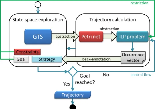
trajectory exploration approach. Apart from the GTS, thestate space explorationcontains agoal, which describes properties of the final state (such as the number of elements of a given type), andconstraintsthat each state must satisfy along the trajectory we seek (e.g. minimum number of elements of a given type). In our approach, both goals and constraints are defined as graph patterns. Finally, the explorationstrategy(including cut-off and selection criteria) is used to decide between multiple possible operations at a given state. The overall objective of the approach is to find atrajectory from the initial state to the final state. In our approach the strategy uses hints retrieved from analysis of the abstracted GTS as described in the following:
Figure 1: Overview of the solution
Occurrence vector-based search strategy approach In [VV06], the computation of an op-timal rule application sequence is performed by encoding the Petri net abstraction (detailed in [VVE+06]) of the GTS into aninteger linear programming (ILP) problem. Thesolutionof this problem (solved using CPLEX1 in our implementation) is a candidate transition occurrence vector. Since the abstraction does not guarantee that this vector corresponds to an executable execution, its feasibility should be checked on the GTS-level. However, in the original approach, the occurrence vector was used in the GTS state space exploration by only allowing occurrence vector compliant execution paths to be explored. Therefore, it did not help in selecting the most promising execution path or cutting the search on infeasible paths.
Selection and cut-off criteria for search strategy In this paper, we propose additional tech-niques, which also use the occurrence vector as a hint, to guide the state space exploration (implemented as an extension to the VIATRA2 model transformation framework [V2]) to further increase the performance of the algorithm. The main features of these new techniques are(a)using the rule (or transition)dependency graph(Gd) computed from the GTS (using the Condor [Con]
dependency analyzer tool) to have a global view on the effects of rule applications [MKR06];(b)
definingselection criteria Crselon the applicable rules (transitions) at a given state (for deciding between alternative upcoming operations); and(c)definingcut-off criteria Crcut on the paths (for deciding about the feasibility of further exploration). Criteria defined in both(b)and(c)depend onGd and the application numbers for the rules (transitions) in the occurrence vector.
3
Definitions
In this section the basics of graph transformation, GTSs and their PN-based abstraction are shortly discussed. Before the definition, we introduce our demonstrating case study.
3.1 Example
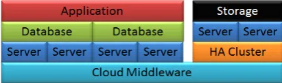
We consider services built on top of acloud middleware(CM) using components as building blocks. Servers(S) and high-availabilityclusters(Cl) can be deployed on the CM, whiledatabases(DB) are installed on servers andapplications(App) are executed over databases. Finally, servers can also be deployed on clusters andstorage(St) subsystems can only operate over clustered servers. Note that the configuration is not a tree structure (e.g. a database is deployed on multiple services, which in turn are deployed on a cloud or cluster), but a directed graph.
In order to provide an appropriate infrastructure for clients, the configuration of the cloud infrastructure must meet certain requirements, e.g. an application and a storage subsystem is required for a cloud-based web service. Such an infrastructure is shown inFigure 2.
Figure 2: An example system providing reliable service
To satisfy this constraint the cloud configuration has to be designed in an appropriate way. We assume that regular change management commands are issued by some middleware service broker. If the current infrastructure of the cloud implies that the required parameters cannot be satisfied by the actual cloud configuration, reconfiguration operations are to be initiated, which lead the system into a state where all constraints are met.
The reconfiguration actions of cloud components will be captured by a graph transformation system that is defined subsequently. An overview on using graph transformations for software architecture reconfigurations can be found in [BHTV06].
3.2 Graph Transformation
typed overT Gby a typing morphismtype:G→T G. Letcard(G,x)denote the cardinality (i.e. the number of graph objects) of typex∈T Gin graphG.
Figure 3: Type graph An example type graph is shown in Figure 3. The type graph
contains only one cloud componentNodedesignated graphically as a rectangle. The edgesCM, Cl, S, DB, AppandStare used to denote the type of the component such that the source and the target node of this edge is the same node (SomeansSocketand represents aCM orCl). EdgeonRconnect two different components denoting that the source node is deployed on the target node of this edge.
Graph transformation (GT) [CMR+97] provides a rule-based manipulation of graph models. A graph transformation (GT) rule typed over a type graphT Gis given byr= (L←−l K−→r R)
whereL(left-hand side),K(context) andR(right-hand side) graphs are typed overT Gand graph morphismsl,rare injective. The negative application conditions (NAC) of a GT rule are given by a (potentially empty) set of pairs(N,n)withNbeing a graph also typed overT Gandn:L→N an injective graph morphism.
Application of a rule rto ahost graph Galters the model graph by replacing the pattern defined byLwith the pattern ofR. This is performed by (i)finding a matchof patternLin modelG(ii) checking the negative application conditions N, which may prohibit rule application, i.e. if there is a match ofNinG(as an extension of the match ofLinG), then the rule is not applicable (iii) removinga part of the modelMthat can be mapped to patternLbut not patternRyielding an intermediate graphDand (iiii)addingnew elements to the intermediate graphD, which exist inR but not inLyielding the derived graphH.
Agraph transformation sequence (GT sequence)is a sequence of GT steps (application of a rule on a given match), i.e., a sequence of rule applications. A GT sequence starting from graph GyieldsG0 and more than one GT step may belong to it. In the paper, we follow theDouble Pushout Approach[CMR+97].
Example1 The ongoing example is captured by a set of graph transformation rules inFigure 4. In order to simplify the graphical presentation, we simply write the typeCM, S, Cl, DB, App, Stof the component on the node (which is denoted by a rectangle) instead of self-loop edges. This way, onlyonRedges remain, which we also omit by representing the hierarchy of deployment using vertical stacking of components.
The addCMrule adds a newCMto the configuration,addScreates a newSdeploying it on top of aCMorCl, however, aClcannot have more than twoSdeployed on it. Rule addClproduces a newCldeploying it on top of aCM,addDbadds a new DBdeploying it on top of two Sthat have no otherNodedeployed on them,addAppcreates a new Appdeploying it on top of twoDBthat have no other Nodedeployed on them. Finally,addStadds a newStdeploying it on top of two S
that are deployed on the sameCland have no otherNodedeployed on them.
Figure 4: Graph transformation rules
GSis defined as a graph where nodes are instance graphs, and edges are graph transformation steps such that the source and target nodes of the edge are graphs.Starting fromG0(initial state) thestate space(i.e. the reachable instance graphs) ofGSis represented taking into account all applicable rules from a given host graph. The different matches of applicable rules may lead to different edges inGS. A path in the graph transition system is aGT sequence also called a trajectory between two graphs. Then we say that a graph is reachable fromG0iff there is a path in theGS.
Example 2 InFigure 5 an extract of the graph transition system of our running example is shown. On the left the root of the graph transition system is the start graphG0where the system configuration contains aCM, threeS, and oneDBcomponents. Rules addS,addCl, and addCMare applicable toG0, here we follow only the application of the first two rules.
3.3 Petri Net Abstraction for GTS
Our guided trajectory exploration approach is based on a Petri net abstraction technique introduced for GTS in [VVE+06]. The motivation behind such an abstraction was that solving the reachability problem on the PN level is of much lower complexity than solving the problem directly on the GTS-level using algorithmic exploration techniques.
The essence of this abstraction technique is to derive a cardinality PN, which simulates the original GTS by abstracting from the structure of instance graphs and only counting the number of elements (nodes or edges) of a certain type by placing tokens to a corresponding place. These tokens are circulated by transitions derived from each GT rule, which simulate the effect of the rule on the number of typed elements by adding and removing tokens from corresponding places.
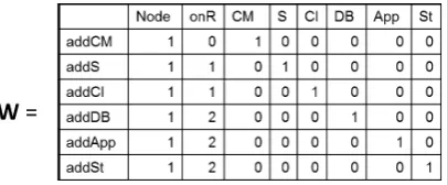
Example3 InFigure 6ruleaddClof our example inSection 3is shown with the corresponding type graph on the left. The PN abstraction is shown on the right. According to the type graph of the example, the corresponding cardinality PN has a place for all node types, namely for type
Node, and edge types, namelyCM, S, Cl, DB, App, St, and onR.
Figure 6: RuleaddCland the corresponding cardinality Petri net
For instance, the left–hand sideLof ruleaddClcontains a node and the edgeCM. Thus the cor-responding transition with the same name has two incoming arcs starting from the corcor-responding places. Similarly, the right–hand side of the rule consists of two nodes and edges CM, Cl, and onR
thus there are four outgoing arcs toNode, CM, Cl, and onRwith weights2,1,1,1, respectively. In this way whenever rule addClis applied the number of the tokens at the involved places changes according to the cardinality of the graph types.
The incidence matrix of the PN abstraction of the example GTS is inFigure 7. The places (columns) refer to the type places corresponding to the type graph ofFigure 6, while transitions (rows) refer to corresponding rules ofFigure 4.
The coverability problem over PN can be encoded into an ILP problem, and the solution of the resulting ILP problem is atransition occurrence vector(σ). The transition occurrence vector
prescribes how many times a GT rule needs to be applied in order to reach the derived submarking of a solution state. For example, to get from an initial graph containing only oneCM to a state with fourSand twoDB, the shortest solution vector would beσ={0,4,0,2,0,0}. Further details
about the encoding and solving can be found in [VV06].
Note that [VVE+06] proves that the mapping is a proper abstraction in the sense that the derived PN simulates the original GTS, and it also discusses a possible abstraction of NACs into cardinality Petri nets. However, that abstraction would deliver an integernon-linearprogramming problem for the trajectory finding problem for which solution techniques have greater complexity than solution techniques for an (I)LP problem. Thus we ignore the abstraction of NACs in the current paper, but it is important to note that this is not a conceptual restriction since NACs only result in the generation of additional infeasible paths.
4
Definition and Usage of the Dependency Graph
In this section we first describe the notion of graph transformation rule dependency and define the dependency graph that is constructed for GTS (Subsection 4.1). Next, we demonstrate how the dependency graph relates to the state of the GTS during trajectory exploration (Subsection 4.2).
4.1 Graph Transformation Rule Dependency
The application of a GT ruler can alter the graph in a way that other rules, which were disabled before, become enabled (or were enabled and become disabled), thus the application of these rules dependon the application ofr. The dependencies between rules are independent of the graph they are applied on, and can be derived from their definition. The analysis can be carried out using various techniques, such as graph matching and graph equivalence (critical pair analysis [HKT02]) or unification and backtracking (conditional transformation-based dependency analysis [Con]), and results in a matrix of dependencies between rules.
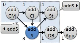
Figure 8: Dependency graph example The result of the analysis is used to create a
depen-dency graph(Gd, illustrated inFigure 8) of the rules,
where eachri is a node (ni) and there is a directed arc
fromnitonj ifrjhassequential dependencyonri(i.e.
the application of ri may affect the match set of rj).
Note that dependencies introduced by NACs are taken into account as well. Finally, there may be arcs in both directions between two nodes.
In this paper, niIdenotes the set of nodes, which
have sequential dependency onni, whileJni denotes
nodes on whichnihas sequential dependency (both sets
illustrated fornaddSinFigure 8).
trajectory calculation, the number of timesrihas been applied in a given path is stored in the application vector(va) asva(i). An execution path of the state space exploration iscompliantwith
σ ifva≤σ(the number of applications is less or equal for each rule). Throughout the paper we
use the difference betweenσ(i) andva(i) (σ(i)−va(i)) as theremaining application numberofri
(#i). This number is stored as an attribute forni inGdtogether with thestate of rithat is either
enabled or disabled in a given GTS state.
Figure 9: GT rule application and its effects on the dependency graph
4.2 Using the Dependency Graph for Trajectory Exploration
The state of the GTS and the dependency graph are tightly connected for a given initial graph and occurrence vector.Figure 9illustrates how the application of a GT rule affects the current graph and the dependency graph. First, the current state is depicted as the graphM(representing the current cloud configuration) and dependency graphGd. The color of the nodes (e.g.naddS) ofGd
represent the state of the corresponding GT rules (raddS), green background for enabled, grey for
disabled. The number near each node is the remaining application number (#addS=3).
In the course of trajectory exploration, the next GT rule, which is applied (raddSin the example)
isselectedfrom the set of enabled rules. Theapplicationhas the following effects on the graphs: (a) graph Mchanges according to the rule definition (here, a newS is added toCM), the new graph is illustrated asM0(b) the #addSismodifiedto represent that the rule is applied (it decreases
from 3 to 2) (c)Gd is also changed toG0d, as #addSdecreased and the applicability of GT rules
may change (hereraddDBbecomes enabled). The trajectory exploration then continues fromM0
by selecting a rule based onG0d.
5
Definition and Calculation of Cut-off and Selection Criteria
strategy. In this section we first give an overview of the criteria types (Subsection 5.1), followed by the definition of the criteria constructing building blocks (Subsection 5.2). Finally, we specify an algorithm for calculating arbitrary criteria over dependency graphs (Subsection 5.3) and illustrate its use on the cloud configuration case study (Subsection 5.4).
5.1 Overview of Cut-off and Selection Criteria
Our guided exploration approach uses the dependency graph as additional information to decide in which order the states of the GTS are explored. In a certain state, two decisions are made regarding the next step, (a) whether the current branch is promising and should be further explored, if yes (b) which enabled GT rule should be executed to reach the next state. We define formal criteria over the current dependency graph, which are evaluated in order to support decisions:
• Cut-off criteria (Crcut) inspect the current state of the dependency graph and return a boolean result, which is true if further exploration of the current branch cannot lead to a goal state with a compliant trajectory. In this case, the exploration continues from another state instead of executing a GT rule in the current state.
• Selection criteria (Crsel)take the dependency graph and define an ordering of the enabled GT rules. A given GT ruleriis placed before another rulerj, if the execution ofriis more
promising, based on the criteria and the current state, than the execution ofrj. The ordering
is used instead of selecting the most promising rule since the exploration may lead to a cut-off on the most promising branch. In this case the next rule in the ordering is executed.
• Soft cut-off criteria (Crso f t)differ from regular cut-off criteria by marking a given branch only unpromising, instead of incompatible. In this case the exploration continues from an other branch, but may return to the unpromising branch if a trajectory to a goal state is not found on other branches.
5.2 Criteria Building Blocks
In our approach, the criteria are constructed using starting point identifiers and a well-defined set of operators (i.e.building blocks), which can represent navigation over the graph edges, numerical and logical functions between subcriteria, ordering of results and quantifiers. Starting points behave asoperandsand create a criteria together with an operator. The resulting criteria (called a subcriteria) can be also an operand to create more complex criteria. Throughout the paper we refer to an operator asenclosingfor the operands which it is combined with. For the definition of the criteria grammar, seeAppendix A. The criteria building blocks are defined in the following:
Starting points identify rules on which a given criteria is interpreted. Trivially, selection criteria are evaluated for rules, which are enabled in the given state and their #i is greater than
zero. However, cutoff criteria may be defined on rules with different properties (e.g. disabled rules or all enabled rules, regardless of #i).
used in logical and numerical functions when one of the operands is a predefined number. Finally, custom starting points([Cr]) are defined when only rules with specific properties are evaluated.
Navigation operators describe which other nodes of graph Gd should be evaluated when
starting from a given node. Navigation is defined over the edges between the graph nodes, and can be limited to paths of one or multiple connected edges. During evaluation, the #j for eachrj
reached by the navigation is summed up, except if navigation occurs in the criterion of a custom starting point, where #jis not incorporated in the total.
For a given ruleri,forwardnavigation (riI) returns the set of nodes to whichri has outgoing
edges, whilebackwardnavigation (Jri) returns the set of nodes from whichrihas incoming
edges. Furthermore, a given navigation operator can be used iteratively on a set of rules either for a given amount of time (limitediteration), e.g. navigating forward twice (riI I) can be defined
asriI2. Finally, a given operator can be used iteratively for as long as it is applicable (transitive
iteration,riI+).
Numerical functions are used when the partial evaluation results of subcriteria are combined. Among the numerical operators, theadditionoperator (Cr1+Cr2, whereCriare subcriteria) is used most often for summing partial results, butsubtraction(Cr1−Cr2),multiplication(Cr1∗Cr2) anddivision(Cr1/Cr2) are also usable.
Logical functions are also defined between two subcriteria and result in boolean values, where the result depends on the actual operator type and the subcriteria operands. For subcriteria, which have numerical results, the available operators areequals(Cr1=Cr2),differs(Cr16=Cr2),more (Cr1>Cr2) andless(Cr1<Cr2).
Similarly, for subcriteria, which have boolean results (e.g. ones that use one of the operators above), the available operators are conjunction(Cr1∧Cr2),inclusive disjunction(Cr1∨Cr2), exclusive disjunction(Cr1⊕Cr2) andnegation(¬Cr).
Ordering and quantifiers are top-level binary operators for selection and cut-off criteria, respectively. Ordering operators define how the numerical results from the subcriteria are returned, with either the highest result being the first (maximaloperator, maxCr) or the lowest (minimal operator, minCr). For cut-off criteria, we define quantifiers to describe when the subcriteria must be true for at least one rule (existentialquantifier,∃r Cr) or for every rule (universalquantifier, ∀r Cr) among the rules defined by the starting point.
Example4 Here, we show the usage of the building blocks using several examples, both for cut-off and selection criteria, which are meaningful when dealing with guided state space exploration. In the rest of the paper, we will illustrate the evaluation of criteria using these examples and the dependency graph from our case study.
can be seen as the only one applied when the guidance is based on the occurrence vector.
Equation 1defines the criterion using the notation introduced in this section.
CrcutNcp:∀r E(r) =C(0) (1)
Permanently disabled rule cut-off criterion The current path can be cut if there is a disabled rule, which still has to be applied based on the transition occurrence vector, but the application of any rule, which it depends on would lead to a non-compliant path.Equation 2
gives the criterion with custom starting points and equally with regular navigation operators.
CrcutPdr:∃r J[D(r)>C(0)] =C(0)or equally∃r(D(r)>C(0))∧(JD(r) =C(0)) (2)
Maximal forward-dependant application path selection criterion Among the applicable GT rules at any given state of the exploration, the one with the most (transitively) dependant rule applications should be executed first (Equation 3). The selection is based on calculating the effect of each applicable rule using the dependency graph and on the idea that a rule, which affects more applications should be applied earlier in the trajectory.
CrselM f d: max E(r)I+ (3)
Minimal backward-dependant application path selection criterion In order to guide the ex-ploration towards a state where one of the cut-off criteria may be applicable, the rule selection is based on calculating the remaining rule applications for backward-dependant rules (Equation 4). In this case, the calculation starts from rules, which depend on the evaluated rule, therefore the result can informally described as the sum of the remaining application number for rules, which affect the same rules as the current rule.
Crselmbd: minJ+[E(r)I] (4)
5.3 Calculation Algorithm for Criteria
InSubsection 5.1, we defined selection and cut-off criteria as means to help the decision whether to explore reachable states on a given branch and which GT rules to execute if we do. These criteria are constructed from the building blocks introduced inSubsection 5.2. In this section we specify the algorithm for calculating arbitrary criteria.
Algorithm overview First, we describe the steps of the calculation for arbitrary criteria (Cr) defined using the building blocks. Let us assume that at the beginning of the algorithm we have a dependency graph (Gd) where the status of the nodes (ni) is updated based on the applicability of
the corresponding rule (ri) and the remaining execution number (#i) is set based onσ(i) andva(i).
functionEVALUATE(Cr,Gd)
initialize variablesLn,Sst,S
check inconsistency of starting points inSst
ifstarting points consistentthen
initializeSnwith nodes satisfyingS
letO←enclosing(S) .list of nodes or cut-off
for alln∈Sndo .Iterate through eligible nodes
initializeNc,Nv,Rp,Rb .Current and visited nodes, partial results
whileO6=Crdo .Evaluation terminates when the applied operator is the criteria APPLYOPERATOR(O,Gd,Nc,Nv,Rp,Rb,Ln) .Apply operator
letO←enclosing(O) .Get enclosing operator
end while
update list or cut-off result
end for
return result
end if end function
1. Check the set of starting points (Sst) inCrto ensure that there is no apparent inconsistency
(e.g. bothE(r)andD(r)is used).
2. Select starting pointSfromSst, this selection may use the first simple or custom starting
point from the criteria or choose randomly. The selection method does not affect the calculation algorithm, however the selected starting point can greatly affect the required calculation steps for specific criteria (e.g. if a custom starting point would rule out the large majority of rules, the rest of the criteria is not evaluated).
3. Acquire the set of nodes (Sn) fromGd which satisfyS (e.g. nodes for enabled rules for
E(r)). IfSis a custom starting point, it can be calculated with the same algorithm (starting fromStep1, whereS:=Cr) to find satisfying nodes.
4. Select the next node (n) fromSnand the enclosing operator (O) ofS. Initialize the set of
current nodes (Nc) including onlyn.
5. ApplyOonNc, where application is based on the type of the operator as follows:
Navigation operators take the current nodes and return nodes, which are reachable in the graph (in the direction defined by the operator) and are not included in the already visited nodes (Nv). These nodes (Nr) are added to theNvand will serve asNcin the
next step (Nc:=Nr). The #iof eachniis summed and added to the partial result (Rp).
Numerical and logical operators are applied as implied by their definition and result in Rpand boolean values (Rb), respectively.
Ordering operators placens in the appropriate position in the list of calculated nodes
Quantifier operators decide whetherCrcut is satisfied based onRb. IfRbis true and the
quantifier isexistential, the current branch is cut and other nodes are not calculated. Similarly, ifRbis false and the quantifier isuniversal, the branch is not cut. In both
cases, skip toStep8.
6. If there is an enclosing operatorOeforO(ifOis transitive andNc6=/0,Oe:=O), applyOe
(continue fromStep5) onNc,RpandRb(whichever exists).
7. If there is a next node (nn) inSn, continue fromStep4(i.e. calculate criteria on next node).
8. ReturnLnfor selection criteria andRbfor cut-off criteria (the branch is cut if true).
Calculation of multiple criteria For more efficient trajectory calculation, several cut-off and selection criteria are defined as the search strategy. The combination of cut-off criteria can be seen as inclusive disjunction (if any of them are true, the branch is cut), while the combination of selection criteria is non-trivial and requires a method for merging different lists.
5.4 Step-by-step Criteria Calculation Example
We illustrate the execution of the algorithm using thePermanently Disabled Rulecut-off and Maximal forward-dependant application pathselection criteria using the cloud configuration case study. Throughout the description of the example we refer back to the steps of the algorithm in parentheses (e.g.S4meansStep4).
Permanently Disabled Rule The calculation ofCrcutPdr is illustrated inFigure 10 using the dependency graph of the example with selected #ifor the rules and the current cloud configuration.
Disabled rules are depicted with light gray background (hereaddStandaddApp), while enabled rules are drawn with green background. The formal definition of the criteria is also included below the graph with partial resultRpin the bottom right corner. The definition has two starting
points, which are consistent (bothD,S1), thus the algorithm chooses the first one asS(depicted with bold circle,S2) then acquiresSn:={addSt;addApp}(S3) and selectsaddStasnand>asO
(S4, 1.inFigure 10).
The application ofOreturns true (S5) therefore the enclosing operator∧is applied next (S6), which means that the second operand has to be evaluated as well. The evaluation of the backward navigation operator (J) is illustrated in 2.ofFigure 10, where the current nodes reached by navigation are depicted with dashed circles (addClandaddSt,S5). Since both #addCl and #addS
is zero, the=operator evaluates to true (S6andS5), the original∧operator returns true as well (S5). Finally, the evaluation of the existential quantifier operator (S5) means that the rest of the nodes are skipped and the branch is cut (S8).
Maximal forward-dependant application path The calculation ofCrselM f d is illustrated in Fig-ure 11similarly to the first example. The configuration of the cloud and the dependency graph are depicted in a different state, and the formal definition of the criteria is below the graph. As before, the first steps of the calculation algorithm select a starting point (E) from the criteria, the first evaluated node (addCl) and the enclosing operator I(S1-4, 1.inFigure 11).
Figure 11: Example evaluation of selection
The nodes reached by the application of the Ioperator areNc:={addSt;addS}(2.in
Fig-ure 11), and the partial resultRpis updated to 4 (S5). Since the enclosing operator is the transitive
navigation (S6), the Ioperator is used in consecutive steps on nodes in Nc. First,addDBis
reached andRp is updated to 5 (S5, 3.inFigure 11), sinceaddSt is already inNv and no new
nodes are reachable from it. Next,addAppis reached fromaddDBandRpis updated to 6 (S5, 4.
inFigure 11). In the following iteration,Ncis empty (no new reachable nodes), therefore the
enclosing operation max is selected (S6). The application of this ordering operator putsaddClin Ln(S5), thenaddSis selected as the next node (S7). Once all the nodes are evaluated the ordered
list (Ln={addCl,addS}) is returned as the final result of the algorithm (S8).
state if at least aStis required in the configuration (or in any configuration where servers have to be deployed on clusters).
Additional Notes on Criteria Calculation The applicability of these criteria highly depends on the structural properties of the dependency graph. First, if most dependencies between rules are bidirectional or if the graph is almost strongly connected, the selection criteria will be less effective. Furthermore, we suggest using transitive closure for path computation as a first approximation, but we believe that more sophisticated algorithms may be defined by handling cycles in the graph differently from simple paths.
6
Related work
The guiding of trajectory exploration based on rule dependency in graph transformation systems is quite novel idea in the field, but similar approaches are not unprecedented in a broader research scope, as described below.
Our trajectory exploration approach can be regarded as an extension of the constraint satisfaction problems over models (abbreviated as CSP(M)) [HV10], which takes GT rules, constraints and goals and searches for solutions that are reachable from an initial model. The criteria calculation defined in our paper serves as a special solver for CSP(M) by substituting regular solvers using simple breadth first search.
Note that our approach is explicitly designed for trajectory exploration and criteria using trans-formation rule dependency are introduced to increase the efficiency of the state space exploration. The approach in [EGLT11] is similar to our approach as it also exploits the dependencies between GT rules with critical pairs analysis. Here, graph transformation systems are enhanced with control flow as well and the dependency information helps in discovering problems, which could occur in runtime.
Model checking approaches to analyze graph transformation systems are similar to our approach as they also perform state space exploration. One can categorize them as inter-preted approaches like [BK02, Ren04, KK06], which store system states as graphs and di-rectly apply transformation rules to explore the state space, andcompiled approachessuch as [SDR04,SV03,EJL06,BRRS08,BS06], which translate graphs and graph transformation rules into off-the-shelf model checkers to carry out verification.
GROOVE [Ren04] is a model checker over graph transformation systems. Its main benefit is the ability to verify model transformation and dynamic semantics through applying CTL model checking on the generated state space of the GTS. It is mainly used for modeling and verifying the design-time, compile-time, and run-time structure of object-oriented systems.
Augur2 [KK06] is a GTS model checker that tackles the complexity associated with independent rules by condensing the entire state space into a single graph with unfolding semantics. It also provides some approximative techniques to deal with infinitely large state spaces, and counterexample-guided refinement of this abstraction.
The complete approach presented in our paper can also be regarded as a directed model checking approach as categorized by [EJL06]. They use (an ad hoc) SPIN encoding and heuristic search for the analysis of graph transition systems.
Baresi et al. [BRRS08] present a model checking solution for graph transformation systems by translating GTS into Bogor models, which can be used for checking Linear Temporal Logic expressions or special-purpose GT rules similar to GROOVE and CheckVML. In [BS06] graph transformation systems are analyzed using Alloy and its tools, which support property checking and finding trajectories to given final states.
It is common in these solutions that they store system states as graphs and directly apply transformation rules to explore the state space similar to our approach. Their main difference is that they use an exhaustive state space exploration to verify certain conditions in the graph transformation system, while our approach relies on guided traversals.
7
Conclusion and Future Work
Guided trajectory exploration, which is a relevant problem when analyzing graph transformation systems, uses hints to reduce the amount of states traversed when looking for trajectories. The hint is used (i) to decide whether a state is a dead-end (cut-off) and (ii) to order alternative directions to increase the efficiency of the traversal (selection).
In the current paper, we defined selection and cut-off criteria for guided trajectory exploration of GTS, and introduced the dependency graph, which combines GT rule dependencies and occurrence vectors. We also described an algorithm for calculating criteria consisting of navigation and computation over the dependency graph. Our approach was exemplified using the cloud configuration problem.
Future work. We plan to specify and develop the complete guided trajectory exploration technique for arbitrary GTS and evaluate its quality against exhaustive exploration techniques. We aim to support guided trajectory exploration in the VIATRA2 model transformation framework. We are also working on defining more sophisticated (problem-specific) criteria and specialized algorithms to increase the efficiency of the approach.
Bibliography
[BHTV06] L. Baresi, R. Heckel, S. Th¨one, D. Varr´o. Style-Based Modeling and Refinement of Service-Oriented Architectures.Journal of Software and Systems Modelling5, 2006.
[BK02] P. Baldan, B. K¨onig. Approximating the Behaviour of Graph Transformation Systems. In Cor-radini et al. (eds.),Proc. ICGT 2002: First International Conference on Graph Transformation. LNCS 2505, pp. 14–29. Springer, Barcelona, Spain, 2002.
[BRRS08] L. Baresi, V. Rafe, A. T. Rahmani, P. Spoletini. An Efficient Solution for Model Checking Graph Transformation Systems.ENTCS213, 2008.
[CMR+97] A. Corradini, U. Montanari, F. Rossi, H. Ehrig, R. Heckel, M. L¨owe.In [Roz97]. Chapter Al-gebraic Approaches to Graph Transformation — Part I: Basic Concepts and Double Pushout Approach, pp. 163–245. World Scientific, 1997.
[Con] Condor, CT-based dependency analyzer.http://roots.iai.uni-bonn.de/research/condor/.
[EGLT11] C. Ermel, J. Gall, L. Lambers, G. Taentzer. Modeling with Plausibility Checking: Inspecting Favorable and Critical Signs for Consistency between Control Flow and Functional Behavior. InFundamental Approaches to Software Engineering. Lecture Notes in Computer Science. Springer-Verlag, 2011. Accepted.
[EJL06] S. Edelkamp, S. Jabbar, A. Lluch-Lafuente. Heuristic Search for the Analysis of Graph Transi-tion Systems. InProc. Third International Conference on Graph Transformation. LNCS 4178, pp. 414–429. Springer, Natal, Brazil, 2006.
[HKT02] R. Heckel, J. M. K¨uster, G. Taentzer. Confluence of Typed Attributed Graph Transformation Systems. InIn: Proc. ICGT 2002. LNCS. Springer, 2002.
[HV10] A. Horv´ath, D. Varr´o. Dynamic constraint satisfaction problems over models.´ Software and Systems Modeling, 2010.
[KE10] B. K¨onig, J. Esparza. Verification of Graph Transformation Systems with Context-Free Specifications. In Ehrig et al. (eds.),Graph Transformations. Lecture Notes in Computer Science 6372, pp. 107–122. Springer Berlin / Heidelberg, 2010.
[KK06] B. K¨onig, V. Kozioura. Counterexample-Guided Abstraction Refinement for the Analysis of Graph Transformation Systems. InTACAS. Pp. 197–211. 2006.
[MKR06] T. Mens, G. Kniesel, O. Runge. Transformation dependency analysis - a comparison of two approaches. In Rousseau et al. (eds.),LMO. Herm`es Lavoisier, 2006.
[Ren04] A. Rensink. The GROOVE Simulator: A Tool for State Space Generation. In Nagl et al. (eds.), Applications of Graph Transformations with Industrial Relevance (AGTIVE). LNCS 3063. Springer-Verlag, 2004.
[Roz97] G. Rozenberg (ed.).Handbook of Graph Grammars and Computing by Graph Transformations: Foundations. World Scientific, 1997.
[SDR04] O. M. dos Santos, F. L. Dotti, L. Ribeiro. Verifying Object-Based Graph Grammars.Electr. Notes Theor. Comput. Sci.109:125–136, 2004.
[SV03] A. Schmidt, D. Varr´o. CheckVML: A Tool for Model Checking Visual Modeling Languages. In´ Stevens et al. (eds.),Proc. UML 2003: 6th International Conference on the Unified Modeling Language. LNCS 2863, pp. 92–95. Springer, San Francisco, CA, USA, October 20-24 2003.
[V2] VIATRA2 Model Transformation Framework, An Eclipse GMT Subproject.http://www.eclipse. org/gmt/VIATRA2/.
[VV06] S. Varr´o-Gyapay, D. Varr´o. Optimization in Graph Transformation Systems Using Petri Net Based Techniques.Electronic Communications of the EASST (ECEASST)2, 2006. Selected papers of Workshop on Petri Nets and Graph Transformations.
[VVE+06] D. Varr´o, S. Varr´o-Gyapay, H. Ehrig, U. Prange, G. Taentzer. Termination Analysis of Model Transformations by Petri Nets. InProc. Third International Conference on Graph Transforma-tion (ICGT 2006). LNCS 4178. Springer, Brazil, 2006.
A
Criteria grammar definition
The following is the BNF grammar used for defining arbitrary criteria:
hcriterioni→ hcut-offi hselectioni
hcut-offi→ hquantifieri hlogicali hselectioni→ horderingi hnavigationi hquantifieri→‘∃’hrulei
‘∀’hrulei horderingi→‘min’|‘max’
hrulei→‘r’[a-z]*
hstartingPointi→ henabledi hdisabledi hconstanti hcustomi
hlogicali→[hnumericali | hstartingPointi]hlogNumOpi[hnumericali | hstartingPointi]
hlogicali hlogBinOpi hlogicali | hlogUnOpi hlogicali hnavigationi→ hnavOpi[hstartingPointi | hnavigationi]
hnumericali→[hnavigationi | hnumercali]hnumOpi[hnavigationi | hnumercali]
henabledi→‘E(’hrulei‘)’
hdisabledi→‘D(’hrulei‘)’
hcustomi→‘[’[hnavigationi | hlogicali]‘]’
hconstanti→‘C(’hnumberi‘)’
hnumberi→[0-9]+
hlogNumOpi→‘=’|‘6=’|‘<’|‘>’|‘≤’|‘≥’
hlogBinOpi→‘∧’|‘∨’|‘⊕’
hlogUnOpi→‘¬’
hnavOpi→[‘J’|‘I’] [‘+’| hconstanti]?
hnumOpi→‘+’|‘-’|‘*’|‘/’
B
Evaluation algorithm
The following is the pseudocode for the criteria evaluation algorithm:
functionEVALUATE(Cr,Gd) .Evaluation of criteria
letLn←φ .Ordered list of nodes
letSst←s:startingPoints∈Cr .Gather starting points
letS←Sst[1] .Select first starting point
fori←2,size(Sst)do .Check all other starting points
ifS6=Sst[i]then .Two starting point is equal, if they are of the same type
letinconsistent←true .Inconsistent criteria cannot be evaluated end if
end for
if¬inconsistentthen
letSn←n∈Gd|S(n)←true .Gather nodes satisfying starting point
letO←enclosing(S) .Get enclosing operator
for alln∈Sndo .Iterate through gathered nodes
letNc←n,Nv←φ .Initialize set of current and visited nodes
letRp←0,Rb←f alse,limit← −1,break←f alse.Initialize partial results, navigation limit and loop break signal
limit←limit(O) .Set limit forlimitedoperators end if
APPLYOPERATOR(O,Gd,Nc,Nv,Rp,Rb,Ln) .Apply operator
ifRp=true∧Cr=cut-off∧quanti f ier(Cr) =existentialthen .Check cut-off condition forexistential
returnRb .Terminate evaluation with cut-off
else
ifCr=cut-off∧quanti f ier(Cr) =universalthen .Check cut-off condition foruniversal
returnRb .Terminate evaluation without cut-off
else
break←true
O←Cr .Force exit from loop at next check
end if end if
ifO=limited∧Nc=6 φ∧limit>1then .If further iterations are required
limit←limit−1 .Decrease limit
else ifO6=transitive∨Nc6=φthen .Nottransitivenavigation or no new reached nodes
O←enclosing(O) .Get enclosing operator
limit← −1 .Reset limit
end if .Otherwise continuetransitivenavigation, if new nodes were reached end while
ifCr=selection∧break=f alsethen .If the criterion is completely evaluated
Ln←Ln∩(Rp,n) .Add result and node to list
Rb←f alse
end if end for
ifRb=f alsethen
ifCr=selectionthen ifordering(Cr) =minthen
Ln←reverse(Ln) .Reverse order formin
end if
returnLn .Return result list for selection
else
returnRp .Return without cut-off
end if else
returnRb .Return with cut-off
end if else
ERROR .Starting points inconsistent
end if end function
functionAPPLYOPERATOR(O,Gd,Nc,Nv,Rp,Rb,Ln) .Application of an operator
ifO∈navOpthen .Navigation functions
letNr←reach(O,Nc,Gd)\Nv .Gather reachable states from dependency graph, excluding already visited nodes
for alln∈Nrdo
Rp←Rp+#n .Update partial result with remaining executions
end for
Nv←Nv∩Nr .Update set of visited nodes
Nc←Nr .Update set of current nodes
else ifO∈logU nOpthen .Unary logical functions
Rb←op(O)Rb
else
letright←EVALUATE(right(O),Gd) .Evaluate right side of criteria
ifO∈logNumOpthen .Logical functions on numbers
Rb←Rpop(O)right .Update boolean result with evaluated value
else ifO∈logBinOpthen .Binary logical functions
Rb←Rbop(O)right
else ifO∈numOpthen .Numerical functions
Rp←Rpop(O)right .Update partial result with evaluated value