Volume 41 (2011)
Proceedings of the
Tenth International Workshop on
Graph Transformation and
Visual Modeling Techniques
(GTVMT 2011)
A visual language for temporal specifications based on Spider diagrams
Paolo Bottoni, Andrew Fish
14 pages
Guest Editors: Fabio Gadducci, Leonardo Mariani
Managing Editors: Tiziana Margaria, Julia Padberg, Gabriele Taentzer
A visual language for temporal specifications based on Spider
diagrams
Paolo Bottoni1, Andrew Fish2
1Dipartimento di Informatica, “Sapienza” Universit`a di Roma, Italy,2School of Computing,
Engineering and Mathematics, University of Brighton, UK
Abstract:
Spider Diagrams are a well-established visual language to specify sets, their rela-tionships, and constraints on their cardinalities. However, they do not support evo-lution of specifications, where one wants to state that under certain circumstances a specification becomes invalid and a new one must be used, nor transformation of specifications, where one needs operators to manipulate specifications. In this paper, we attack the first problem by developing a new system of timed Spider Diagrams which allow modellers to indicate the temporal range of validity of a specification. The approach is illustrated with examples of policies for library management.
Keywords:Visual constraint language, Time based systems, Spider diagrams.
1
Introduction
Spider Diagrams (SDs) are a diagrammatic logical specification and reasoning system built on top of Euler Diagrams (EDs), suitable for expressing monadic first order logic with equality statements [STHT04]. Constraint Diagrams [Ken97, FFH05] are an extension of SDs which are more expressive (introducing explicit syntax for the expression of quantification and rela-tions), but come with the trade-off of more complexity in interpretation. They were proposed as a means for expressing constraints within software system modelling, potentially as a replace-ment for the textual Object Constraint Language (OCL) within the Unified Modeling Language (UML). These diagrams can be used to specify static constraints over the model such as a system invariant, or behavioural specifications in the form of pre and post-condition contracts. An ad-vantage of using diagrammatic constraint languages is that users become able to display a logical proof as a sequence of diagrams, thereby enhancing confidence in its correctness.
constraints by annotating Spider diagrams with temporal constraints on their validity, and dis-cuss its properties. We provide a semantics for Timed SDs based on a natural representation of the evolution of the state of a system over an interval as a sequence of snapshots and use such a representation to check the consistency of policies specified through several diagrams, possibly presenting overlapping intervals. Besides developing the basis for such definitions, we use them to check if a diagram over an interval in a timed-SD-sequence is a valid instance of a model, or if it is a valid deduction from some such instance (exploiting standard inference figures for SD, as for example those in [HST05]). The proposed model can also be used to derive transformation rules from policies, to simulate the behaviour of processes complying with them, thus allowing both a static and a dynamic analysis of a specification. This opens new avenues of research, such as: (i) the expansion of diagrammatic logic results into a temporal setting; (ii) the translation of the underlying model of the temporal constraint language into a graph transformation setting.
In what follows, Section2introduces new notions of SD-specifications and instances used for modelling, their interpretations and the notion of an SD-instance satisfying a SD-specification. We introduce concepts related to intervals and interval specifications in Section3, and introduce timed-SDs in Section4, providing a notion of SD-stories and semantics of timed-SDs in terms of SD-stories. Finally, Section5discusses related work, whilst Section6draws conclusions.
2
Specialisation of SDs for modelling purposes
We adopt a variant to a standard definition of SDs and of their interpretation (see [HMT+01, HST05]), providing a more direct relation of SDs to modeling in object-oriented terms.
A (concrete) ED is a collection of (labelled) simple closed curves in the plane, called contours, decomposing it into connectedminimal regions. Azoneis a region inside one set of contours and outside all the other ones; zones may beshaded. A (concrete) SD is an ED together with extra syntax forspiders. These are trees whose vertices (calledfeet) are placed in zones, with no two vertices of the same tree lying within the same zone. All diagrams have a “boundary contour”, drawn as a rectangle and labelled byU (the universe of discourse); all regions are then insideU. A concrete diagram represents logical statements according to the following intuitive seman-tics. The interior of a contour represents a set (corresponding to the label) and the regions formed by taking intersection, union and complement of regions represent the result of the corresponding set operations. Spiders represent elements in the sets determined by their habitat (the smallest region containing the spider). Distinct spiders represent distinct elements.Shadingplaces upper bounds on the cardinality of sets: there are no more elements in the set represented by a shaded zone than the number of spider feet touching that zone; a shaded zone without feet touching it represents an empty set. A single diagram is calledunitary. Unitary systems can be extended to compoundsystems, allowing standard logical connectives between diagrams.
Active
admin
Suspended Banned
reader
WithLoan IsIdle
Active
reader admin
Figure 1: An example of two SD-specifications, stating two policy rules for a library.
Definition 1 Let C and S be disjoint sets of labels. Aunitary spider diagram d on L = C∪S is a tuple(C,Z,sh,S,h)such that:Cis a set of curve labels drawn fromC, withU∈C;Z is a set of zones, each of which is defined asz= (X,Y), where the setsXandY form a partition ofC(withU∈X andY possibly empty). X is referred to as theinsideset of curves, andY is theoutsideset;sh:Z→Bis ashadingfunction assigning a boolean value to each zone. A zone zfor whichsh(z) =trueis said to beshaded andZ∗⊂Z denotes the set of shaded zones;S is a set of spider labels drawn fromS;his ahabitat functionh:S→P(Z)that records the set of zones that each spider touches. Each unique pair(s,z)∈S×Z s.t. z∈h(s)is called afoot of spiders, and we callF the set of all feet. Acompound spider diagram,D, is any unitary SD or any construct with unitary SDs as primitives and allowing the unary logical negation operator not, and the binary logical conjunction and disjunction operators∧and∨as connectives.
We provide a standard notion of interpretations and models (in a logic sense); see [HST05].
Definition 2 Letdbe a SD onL. Aninterpretationofdis a pair(U,ψ), whereU is a set and ψ is a function that assigns subsets ofU to each curve. The mapψ naturally extends to zones,
and is also extended to spiders by mapping them to singleton subsets1ofU. An interpretation is amodelfordif it satisfies thesemantics predicate, which states that: missing zones represent the empty set; each spider represents a unique element in the set represented by its habitat; shaded zones have cardinality at most the number of spiders touching that zone.
We distinguish between SDs used for system (invariant) specification and SDs used as model instances. However, we use the same syntax, with restrictions on the form of the labels. We situate SDs within object oriented specifications, with reference to a type system, assuming ac-cess to types, classes, and instances via labels. We interpret SD-specifications and SD-instances by specialising Definition2, varying the interpretation ofψon spiders in the two cases: for
SD-specifications a spider represents a set of objects of a given type, whilst in an SD-instance a spider represents the singleton set containing the named object of a given type. Thus, SD-specifications place global constraints on a model (in a Software Engineering sense) instance.
Definition 3 An SD-specification is an SD, where C is drawn from the set of class or state names of the system andS from the set of types. AnSD-instanceis an SD, whereC is drawn from the set of class or state names of the system, andS are pairs of object names and types. Withd an SD-specification andd0 an SD-instance, aninterpretation ofd ord0 is a pair(U,ψ)
whereUis restricted to be a set of objects of the system, andψmaps curves to the set of objects
ofU of a certain class (as determined by the curve label). For an interpretation ofd,ψ maps
each spider to the set of objects of type indicated by its label. For an interpretation ofd0,ψmaps each spider to the singleton set containing the object with name and type specified by its label.
2.1 Satisfaction
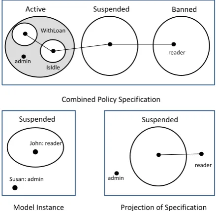
For an SD-instance to satisfy an SD-specification, the spiders in the instance must only inhabit zones corresponding to those inhabited by spiders of that type in the specification, and no con-straint on zone cardinality can be violated. Parts of the specification may be not relevant to the check, e.g. curves not present in the instance. Hence, a projection of a diagramdonto a setC, of abstract curves produces a diagramdC with all curves not inCremoved. This operation, be-sides redefining zones and their shading, modifies accordingly the habitat of spiders, coherently with the adopted semantics for these pieces of syntax. In Figure2(top) an SD-specification d combines the two policies in Figure1. On the bottom left, an SD-instanced0indicates that the in-stanceJohnof typereaderis suspended. The bottom right shows the projectiond{U,Suspended} ofd onto the curve set of d0. As d0 has a correctly typed individual (John and Susan) in an admissible zone for each type ind{U,Suspended}, we say thatd0satisfies d.
Active Suspended
WithLoan
IsIdle
Banned
admin
reader
Suspended
John: reader
Model Instance
Combined Policy Specification
Suspended
admin
reader
Projection of Specification Susan: admin
Figure 2: An example of an SD-instance.
The projection ofd with respect toCis the diagram, denoted dC, obtained fromd as follows: (1) we replace each zone ofd, and each spider ofd, by their projection with respect toC; (2) if z∈Z(dC)thenzis shaded if and only if every zonez0∈Z(d)such that(z0)C=zis shaded.
When considering an SD-instance satisfying an SD-specification, we allow multiple spiders of the same type in the instance, but insist that they all satisfy the constraints from the SD-specification. We also insist that in the SD-instance there is at least one spider of each type present in the SD-specification; moreover, given a spider in the SD-instance, its habitat is con-tained in the projection of the habitat of the spider for that type in the SD-specification.
Definition 5 Let d1 be an SD-specification and let d2 be an SD-instance2. We say that d2
satisfies d1, denotedd2|=d1, if: 1)C2⊆C1; 2)Z2⊆(Z1)C2; 3) Z2∗⊆(Z1∗)C2; 4)(Z∗1)C2∩(Z2\
Z2∗) =/0; 5)π2(S2) =S1, whereπitakes thei-th component of a tuple and is extended to sets; 6)
∀s2∈S2[∃s1∈S1[π2(s2) =s1∧h2(s2)∩Z1C2⊆h(s1)C2]].
3
Interval specifications
We extend SDs to enable temporal specifications, associating temporal annotations with the elements of a SD or with a whole SD, to indicate the time over which the associated con-straint/situation holds. While several models of time could be utilised, we choose to use a model based on calendar time, where consecutive integer indexes are used to indicate contiguous time-intervals each with a duration defined by agranuleor time-unit. The intervals we associate with diagrams have integer endpoints and are interpreted as the sequence of consecutive granules in-dexed by the integers within the interval, including the endpoints. We are interested in themeet, during, andoverlap relations of Allen’s interval algebra [AF94], and they are adapted for use with the intervals associated with the diagrams. One can do this by considering Allen’s relations for the actual time-intervals that are the union of the time-intervals of the consecutive integers in the interval associated to the diagram. The simple set-up presented here essentially combines the model of [AF94] with the calendar model adopted in [BBF01].
We useNto denote the set of natural numbers andN0forN∪ {0}. For the granularity of
in-tervals we consider standard time units e.g. seconds, hours, days, with the usual layering among them. Hence, each granule can be decomposed into finer sub-granules up to some undecom-posable granule (i.e. our time model is ultimately a discrete one). However, we consider that significant specifications are expressed with respect to decomposable granules. Time 0 refers to the system starting time for the model at hand.
Definition 6 Given a time unitu, leta,b∈N0 anda≤b. We call[a,b]u thetime interval in u, i.e. the ordered sequence of granules indexed by all natural numbers between and includinga andb. The set of all time intervals inuis denoted byIu. WithI1= [a1,b1]u,I2= [a2,b2]u∈Iu,
we say: 1)I1meets I2, denoted byI1uI2, iffa2=b1+1; 2)I1during I2, denoted byI1vI2 iff
2For simplicity we assume here that these are unitary diagrams and that the SD-instance does not contain curves that
a1≥a2,b1≤b23; 3)I1overlaps I2, denoted byI1tI2, iffa1<a2≤b1<b2. If none of the above
occurs, we say thatI1andI2aredisjoint, with the two casesI1<I2andI1>I2. For non disjoint I1andI2, we define theirmerge I1I2as the intervalI = [min(a1,a2),max(b1,b2)].
Example 1 We have[0,2]du[3,6]d; they merge to give [0,6]d. In this case we use days as granules, so the interval specifies the 7 consecutive days of a week; the interval[1,1]d, with the same start and end point, is interpreted as the second day of the week, starting counting at 0. We also have[1,2]dv[1,4]d, and[1,2]d[1,4]d= [1,4]d;[1,3]dt[2,4]d and[1,3]d[2,4]d= [1,4]d;[1,2]d is disjoint from[4,5]d.
Besides simple intervals, we have interval specifications involving expressions on variables.
Definition 7 Given a time unit u, an interval specification in u is a construct [exp1,exp1+ exp2]u, whereexp1andexp2are two linear expressions including natural numbers and variables
(with integer coefficients other than zero) that can be evaluated overN0. Var(exp) denotes the
set of variables appearing inexpandVar(I)the cumulative set of variables fromexp1andexp2. A valuationVal(exp)is a set of assignments to natural numbers for each variable inVar(exp), so that each occurrence of the same variable name is assigned the same value. AnalogouslyVal(I)
denotes the simultaneous valuation ofexp1andexp2. The value ofexpaccording toVal(exp)is denotedkVal(exp)k. Theinterpretationof an interval specificationtSpec= [exp1,exp1+exp2]u
is the set of intervalsint(tSpec) ={[a,b]u∈Iu| ∃Val(tSpec),s.t.kVal(exp1)k=a,kVal(exp2)k =b−a}. We denote byIu0the set of interval specifications inu.
Example2 Consider an interval specificationI= [x+1,x+1+2y]u. ThenVar(x+1) ={x}, Var(2y) ={y}, andVar(x+1+2y) ={x,y}=Var(I)are sets of variables. Suppose that we have valuation functionsVal(x+1)such thatx7→3, andVal(2y)such thaty7→1. Thenx7→3,y7→1is an assignment of natural numbers to variables inVar(I). The values of the expressions according to these assignments are: ||Val(x+1)||=4,||Val(2y)||=2,||Val(x+1+2y)||= 6,||Val(I)||= [4,6]u. The interpretation of[x+1,x+1+2y]uis the set of all intervals[a,b]us.t.a≥1andb−a is an even number (possibly 0). Note that each valuation of an interval specification,I, fixes it to be a specific interval.
In the following, we omit the indication of the unit where no ambiguity arises, and deal only with specificationstSpecs.t. int(tSpec)6=/0, ruling out specifications such as[x,x−(2x+1)]. Two non disjoint intervalsI1,I2in a set of intervalsIcan be naturally decomposed into a sequence
of at most three contiguous intervals (i.e. meeting and not overlapping) as follows: 1) ifI1uI2
do nothing; 2) if I1vI2 (and it is not the case thatI1 starts, finishes or is equal toI2, hence a1>a2 and b1<b2) then build the sequence [a2,a1−1],[a1,b1],[b1+1,b2](the other cases
being easily derivable); 3) ifI1tI2, then build the sequence[a1,a2−1],[a2,b1],[b1+1,b2]. This
procedure can be iterated on any set of intervals (s.t. no interval is disjoint from all the others) until each non disjoint pair of intervals meet. It can be proved that the resulting collection of intervals is unique. Note that this does not create new end or start points other than those in the set{a2−1, . . . ,an−1,b1+1, . . . ,bn−1+1}. Also note that some intervals can be reduced to a
unitary interval, e.g ifa2−1=a1 for case 2) above. We extend the decomposition concept to
interval specifications.
Definition 8 LetI={I1, . . . ,In}be a finite set of intervals, forIi= [ai,bi]∈I, s.t. J
i∈{1,...n}Ii
is defined and equal to[min(ai),max(bi)]fori∈ {1, . . . ,n}. Anon overlapping coverofI is a
finite set of intervalsJ={J1, . . . ,Jm}, withJk= [ck,dk], s.t.: 1)Ji∈{1,...,n}Ii=Jj∈{1,...,m}Jj; 2)
for eachk∈ {1, . . . ,m−1},JkmeetsJk+1(i.e. ck+1=dk+1).Jis thecanonical non overlapping coverif its set of intervals coincides with the one derived from the procedure described above. LetI0={I10, . . . ,In0}be a finite set of interval specifications, and letVal be a valuation function forI0(i.e. for all of the interval specifications inI0). Then a(canonical) non overlapping coverof I0w.r.t.Valis a finite set of interval specificationsJ0={J10, . . . ,Jm0}s.t.kVal(J0)kis a (canonical) non overlapping cover ofkVal(I0)k.
Example 3 Suppose that I ={I1 = [1,5],I2 = [4,5],I3 = [2,9]}. Then J
i∈{1,2,3}Ii = [1,9]. Let J ={J1 = [1,1],J2 = [2,3],J3 = [4,5],J4= [6,9]}, so Jk∈{1,2,3,4}Jk = [1,9] andJ is the canonical non-overlapping cover ofI. On the contrary,J0={[1,2],[3,4],[5,6],[7,9]}is another non-overlapping cover, which is not canonical as can be easily seen since 7 is an endpoint ofJ0
not in the set{1,2,3,4,5,6,9}.
4
Timed Spider Diagrams
We introduce timed SDs as associations of SDs with specifications of admissible time intervals for elements in a diagram and with constraints on variables appearing in the specifications. They can express fairly complex temporal relations and we wish to facilitate operations such as the combination of compatible timed-SDs (e.g. stating two parts of a same policy).
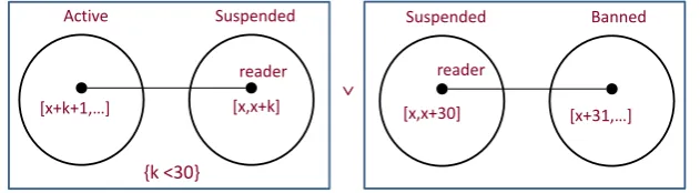
Figure3shows a compound diagram and introduces variables in SD-specifications. Variables are used to specify intervals which can start at any time, so that a designated variable is instan-tiated to define the onset of the interval. Variables are bound to natural numbers, and subject to constraints. The figure refines the library policy: a user who stays in theSuspended state for a whole period of 30 days (for example for not paying a fine) becomes banned. In this case the designated variablexcan be instantiated at any time, in correspondence with the moment where a user enters theSuspendedstate, while the use ofkand of the associated constraint indicates that being in this state may cease at any time before the deadline of 30 days4. We consider time-valid diagrams where elements are present only if elements on which they depend are also present, e.g. a foot can be in a zone only during the existence interval for that zone.
Definition 9 Atimed SD is a constructdT = (d,ω,X), where d= (C,Z,sh,S,h) is an SD,
ω:C∪Z∪(Z×B)∪S∪F→I0is a function assigning an interval specification to each object5
ind, andX is a set of linear constraints on the valuations for the specifications assigned byω,
where all instances of variables with the same name receive the same value. LetVal(ω) be
a valuation function that consistently evaluates every variable in the image ofω. A valuation
4For simplicity, we omit here the indication of the time unit.
Suspended
[x,x+k]
{k <30}
Active
[x+k+1,…]
Suspended Banned
reader
[x+31,…] [x,x+30]
reader
Figure 3: A user either exits from suspension within 30 days or becomes banned.
kVal(ω(x))k= [a,b]satisfiesX, denotedkVal(ω(x))k |=X, if no assignment inValviolates a
constraint inX, anda≤b. We say thatdT istime-validif∃Val(ω)s.t.:
1. ∀x∈C∪Z∪(Z×B)∪S∪F[kVal(ω(x))k |=X].
2. The following general constraints hold:
• ∀f = (s,z)∈F[kVal(ω(f))k v kVal(ω(s))k];
• ∀f = (s,z)∈F[kVal(ω(f))k v kVal(ω(z))k];
• ∀z∈Z[kVal(ω(z,sh(z)))k v kVal(ω(z))k];
• ∀z∈Z,c∈C[kVal(ω(z))k v kVal(ω(c))k].
Given an interval specification [exp1,exp1+exp2], if there exists a variable x∈Var(exp2)\
Var(exp1), s.t. no constraint is explicitly given forx, then we say thatexp1+exp2isunlimited
and write[exp1, . . .]. In the following, we only deal with time-valid diagrams, and rule out
in-admissible sets of specifications, such asI={[x,x+y],[z−y,x−z−1]}withX={y=z,z=2x}. Elements in a diagram are present during the specified time-intervals, with any non-assigned element being assigned[0, . . .]by default. We interpret that for any intervalI disjoint from the image of a diagram element, that element is not present duringI. Note that associating an interval with a pair inZ×Ballows for modifications over time of the property of being shaded for a zone. A timed-SD(d,ω)can represent a complex time-based set of constraints. However, this can
be reduced to a collection ofbasic timed SDs where each diagram is associated with a single interval. This construction is possible ifω is well-defined for every element ofdand the image of any such element underω is a single interval. Hence, for each time-valid timed SD there
is an equivalent sequence of basic timed SDs, where the intervals of consecutive diagrams are contiguous. In Definition10, we first define these concepts for SDs, permitting specialisation to SD-specifications and SD-instances, and then we make use of specialisations by providing semantics to the timed SD-specifications.
Definition 10 (1) Abasic timed-SDis a tuple(d,I,X), wheredis an SD,I∈I0andX is a set of linear constraints onVar(I). (2) Lethdi=h(d1,I1,X1), . . . ,(dn,In,Xn)ibe a sequence of basic
A timed SD encapsulates complex temporal constraints. For purposes such as to allow mod-ularisation of the constraints according to some time-line, as well as defining the semantics of timed SD-specifications, we provide a conversion from timed-SDs to sequences of contiguous basic timed-SDs. The following can be applied to SD-specifications or SD-instances.
Definition 11 LetdT = (d,ω,X)be a time-valid timed SD w.r.t. a valuation functionVal(ω).
Let hd0i=h(d01,J1,Y1) , . . . , (d0m,Jm,Ym)i be a sequence of basic timed SDs, andVal0 a joint
valuation function over theJi’s s.t.: (i)hd0iis contiguous w.r.t.Val0; (ii) for each subintervalIof
kVal0(Ji)k,d0i consists of exactly the diagram elementsxofdfor whichIv kVal(ω(x))k. Then d0 is atime-decompositionofdT. Ifmis minimal subject to (i) and (ii), thend0 is acanonical time-decompositionofdT.
Algorithm 1 LetdT = (d,ω,X)be a time-valid timed SD, and letValbe a valuation function
overω. Then: 1) LetI be the set of all of the interval specifications obtained asω(x), for any x∈C∪Z∪(Z×B)∪S∪F. 2) ConstructJ={J1, . . . ,Jm}, the canonical non overlapping cover
ofIw.r.tVal. 3) Constructh(d1,J1,Y1), . . . ,(dm,Jm,Y1)i, wherediis the SD consisting of the set
of diagram elementsx, for allx∈C∪Z∪(Z×B)∪S∪Ffor whichkVal(Ji)kis not disjoint from
kVal(ω(x))k.
Theorem 1 Let dT= (d,ω,X)be a time-valid timed-SD, and let Val be a valuation function overω. Then the constructh(d1,J1,Y1), . . . ,(dm,Jm,Y1)ifrom Algorithm1 is acanonical
time-decompositionof dT.
Proof. Post-valuation, one can consider the set of intervals associated to each diagram element, and decompose this into a sequence of contiguous intervals which collectively merge to yield the whole timeline. Then, for each interval in this decomposed timeline, there is a single corre-sponding diagram (comprising all and only the diagram elements ofdthat are present within that interval); each of these is a well-defined diagram sincedTis time-valid. These diagrams together
with associated intervals constitute a contiguous sequence of basic timed-SDs. It follows that they form a canonical time-decomposition ofdT, due to the construction. The argument lifts
from intervals to interval specifications.
4.1 Satisfaction and semantics of timed-SDs
Definition 12 Lethdi=h(d1,I1,X1), . . . ,(dn,In,Xn)ibe a contiguous sequence of basic timed
SD-specifications, and lethd0i=h(d10,J1,Y1), . . . ,(dm0,Jm,Ym)ibe a contiguous sequence of basic
timed SD-instances. Then, for a common valuation functionVal, over I1, . . . ,In,J1, . . . ,Jm and
an interval K, we say that: (i) hd0i |=K hdi, if for i,j s.t. K,kVal(Ii)k, and ∩
Val(Jj)
are jointly overlapping,d0j |=di; (ii)hd0isatisfies d, denotedhd0i |=hdi, if∀Ji ∈ {J1, . . . ,Jm}, we
havehd0i |=Jihdi. LetdT = (d,ω,X)be a time-valid timed-SD-specification (w.r.t.Val) and let
hd00i=h(d100,K1,Z1), . . . ,(d00p,Kp,Zp)ibe a time-decomposition ofdT (w.r.t.Val00). Then, for a
common valuation functionVal0overK1, . . . ,Kp,J1, . . . ,Jm,hd0isatisfies dT ifhd0isatisfieshd00i.
Definition 13 LetdT= (d,ω,X)be a time-valid timed-SD-specification. Lethdi=h(d1,I1,X1), . . . ,(dn,In,Xn)i be a contiguous sequence of basic timed SD-instances, s.t. for each valuation
functionValofω, there is an extension ofValtoVal2, a valuation ofω,I1, . . . ,Inwithhdi |=dT,
w.r.t.Val2. Thenhdiis called adT-story and thesemanticsofdT is the set of alldT-stories. We
also speak of SD-stories whendT is implicit.
Suspended
[x,x+k]{k <30} reader
Active
[x+k+1,...] reader
Banned
[x+31,...] reader Suspended
[x,x+30] reader
Figure 4: (a) Alternative cases which are contiguous basic timed SD-specifications for the timed SD-specification of Figure3.
Suspended
[21/3/2009, 21/3/2009 + 30] John: reader
Suspended
[21/3/2009 + 31, 21/3/2009 + 34] John: reader
Figure 4: (b) A contiguous sequence of ba-sic timed instances which is not an SD-story for the specification of Figure3.
Figure4(a) shows examples of two contiguous sequences of basic timed SD-specifications that encapsulate the alternative cases of the timed SD-specification of Figure3. Figure4(b) shows an example of contiguous sequence of basic timed SD-instances which does not satisfy either of the sequences in Figure4(a), and is not an SD-story for Figure4(a); note that if the Suspended state in the second diagram were changed to aBanned state, then this would by a story for the SD-specification in Figure4(a).
Theorem 2 Let dT = (d,ω,X)be a time-valid timed SD-specification, w.r.t. Val, a valuation
function over ω. Let hd0i=h(d10,I1,X1), . . . , (d0n,In,Xn)i be a contiguous sequence of basic timed SD-instances that satisfies a canonical time decomposition of dT. Thenhd0iis an SD-story (called acanonical SD-story).
Proof. Satisfaction of a canonical time decomposition ofdT implies satisfaction ofdT.
Corollary 1 Each time-valid timed SD-specification dT= (d,ω,X)has a non-empty semantics.
Proof. SincedT is time-valid, there is a canonical time decomposition ofdT. Any SD-instance
which realises the spider types of this canonical time decomposition as appropriate (name,type) pairs is an SD-story, as required6.
Definition 14 Aninitialised canonical time decomposition ofdT is a canonical time
decom-position ofdT, w.r.t. a valuation function IVal, which assigns the minimal admissible value to iexp1, withJ1= [iexp1,iexp1+iexp2]. Aninitialised left-minimal canonical time decomposition is an initialised canonical time decomposition with valuationILMVal such that the lengths of eachJiis minimal over allIValvaluations, miminizing in order of increasing indexi.
Theorem 3 Let dT = (d,ω,X)be a time-valid timed SD, and let Val be a valuation function overω. Then there exists a unique initialised left-minimal canonical time decomposition.
Proof. Existence derives from Theorem2, uniqueness from the minimization process.
Theorem 4 Let dT be a timed-SD specification. Then the time-validity of dT is decidable.
Proof. The interval specification constraints reduce to a system of linear diophantine equations (relating end-points to start-points) under a set of constraints. That the solution, without con-straints, is decidable is a classical result.
5
Related work
Several models of time have been proposed for formal specifications, both in relation to real-time [GB03,AD94] or hybrid [Hen96] behaviours. Time-based extensions have been also pro-posed for calculi or specification languages of concurrent processes (see [FOP09] or [BW03]). In general, these models deal with intervals to model uncertainty about the actual occurrence of an event. In Statemate, also a clock-synchronous semantics is provided where events can only occur when a clock ticks [EJW02]. This view was adopted also in [GVH03] to integrate time in graph transformations, by introducing a specific attribute updated by clock messages to processes.
In UML, a simple model of time is adopted, based on a notion of observation, and able to express durations and deadlines [OMG10], whereas in the profile for real-time applications, effects connected with latencies in observation can be taken into account [OMG05]. In both cases, OCL constraints can incorporate conditions on time expressions.
In general, we are interested here in the persistence in a state over a period as dictated by time-dependent policies, rather than in modeling the occurrence of specific transitions triggered by any type of events. As a consequence, the model of time adopted here is connected to the notion of calendar time, as adopted in the area of temporal databases and temporal rule based access control. In particular, we adopt a model analogous to that Bertinoet al. [BBF01], based on a formalism proposed by Niezette and Stevenne [NS92], which however considered intervals of fixed length, repeated after some time. In Bertino’s model a calendar is a set of contiguous in-tervals, each with its own duration, containing all the instants between its extreme granules, from the start of the first granule to the end of the second one. Based on this, they introduce periods to express that some roles have to be granted specific access rights at recurring times. Ninget al. exploit the notions of calendars and granules to define a calendar algebra, where operations allow the grouping of intervals or the subdivision of granules [NWJ02]. Of interest here is the notion that the intervals covered by distinct granules (at the same level) cannot be interleaved. Others consider calendar times as corresponding to an instant, rather than a granule [K ¨O95]. A vast examination of the problems related to the use of different granularities is in [EM05].
The field of multimedia is another area in which the modeling of time is relevant, in particular as sequential media (typically audio and video) may have to be synchronised with the presence of static documents for some time. In many cases one is therefore interested in considering durations of intervals which can start at any point in time, rather than at specific instants. As an example, Bowmanet al.have defined a formalism in which, once a starting point for the system is set, reasoning can be performed on the occurrence, within the current interval, of a state, based on the lengths of the current and previous intervals [BCKT03].
In addition to considering intervals, in the approach presented in the paper, the use of in-stants in the specification of rules can provide a weak form of clock-synchronous specification, associated with the triggering of a time-dependent transition.
In the field of SDs, to our knowledge this is the first attempt to integrate time-related as-pects in the formalism. Moreover, we draw a more precise correspondence with object-oriented modeling, by distinguishing specifications from instance models and providing two distinct in-terpretations for spiders, as types and as typed individuals. A relation can be drawn with the construction of parallel models inZfor constraint diagrams in [HS05].
The idea of representing system dynamics through sequences of EDs was introduced in [BF10], to follow the evolution of sets (rather than the state of individuals) under the effect of a Reaction Systems [ER07], and colour was used to assist in tracking families of sets through the sequences.
6
Discussion and conclusions
However, a limited form of dynamics can be provided by the use of rules enforcing modifica-tions in the state of individuals according to a policy. In this case, we could specify rules over timed specifications, to produce dynamic views of a specified system. To this end, we could use rules triggered by the onset or offset of an interval (in this case making reference to the mapping of intervals onto the fundamental granule layer). For example, given a collection of specifica-tionsh(d1,ω1), . . . ,(dn,ωn)iannotated with contiguous interval specifications, one can derive a
collection of rules as pairs((di,ωi),di+1), together with some mappingµ from elements ofdito
elements ofdi+1. The interpretation of such a rule would be that if a system has been described
by an SD instance satisfyingdiover an interval given by a valuation ofωi, then at the end of this
interval it moves to a state described by an SD instance, related to the previous one viaµ, which
is a model fordi+1.
We plan to extend this work in a number of directions. Firstly, standard notions and results from the theory of (static) SDs have to be reviewed and lifted to timed SDs, taking into account the distinction between spiders at the different levels. Secondly, the extension to real-time may require a different basis for time, considering open intervals over the reals. Thirdly, we plan to consider different types of dynamics, integrating event-based and time-dependent specifica-tions, exploiting the mapping of SDs to typed attributed graphs, calledSpider Graphs, presented in [BFP10], possibly following the approach in [GVH03].
Bibliography
[AD94] R. Alur, D. L. Dill. A Theory of Timed Automata.TCS126(2):183–235, 1994.
[AF94] J. F. Allen, G. Ferguson. Actions and Events in Interval Temporal Logic. J. Log. Comput.4(5):531–579, 1994.
[BBF01] E. Bertino, P. A. Bonatti, E. Ferrari. TRBAC: A temporal role-based access control model.ACM Trans. Inf. Syst. Secur.4(3):191–233, 2001.
[BCKT03] H. Bowman, H. Cameron, P. King, S. Thompson. Mexitl: Multimedia in Executable Interval Temporal Logic.Formal Methods in System Design22:5–38, January 2003.
[BF10] P. Bottoni, A. Fish. Coloured Euler diagrams: a tool for visualizing dynamic systems and structured information. InProc. Diagrams 2010. LNAI 6170, pp. 39–53. 2010.
[BFP10] P. Bottoni, A. Fish, F. Parisi-Presicce. Preserving constraints in horizontal model transformations.GTVMT-2010, ECEASST29:1–14, 2010.
[BW03] V. Bulitko, D. C. Wilkins. Qualitative simulation of temporal concurrent processes using Time Interval Petri Nets.Artificial Intelligence144(1-2):95 – 124, 2003.
[EJW02] R. Eshuis, D. N. Jansen, R. Wieringa. Requirements-Level Semantics and Model Checking of Object-Oriented Statecharts.Requir. Eng.7(4):243–263, 2002.
[ER07] A. Ehrenfeucht, G. Rozenberg. Events and modules in reaction systems. TCS 376:316, 2007.
[FFH05] A. Fish, J. Flower, J. Howse. The Semantics of Augmented Constraint Diagrams. JVLC16:541–573, 2005.
[FOP09] M. Falaschi, C. Olarte, C. Palamidessi. A framework for abstract interpretation of timed concurrent constraint programs. In Proc. PPDP ’09. Pp. 207–218. ACM, 2009.
[GB03] H. Giese, S. Burmester. Real-Time Statechart Semantics. Technical report tr-ri-03-239, University of Paderborn, 2003.
[GVH03] S. Gyapay, D. Varro, R. Heckel. Graph Transformation with Time. Fundamenta Informaticae1:1–22, 2003.
[Hen96] T. A. Henzinger. The Theory of Hybrid Automata. InLICS. Pp. 278–292. 1996.
[HMT+01] J. Howse, F. Molina, J. Taylor, S. Kent, J. Gil. Spider Diagrams: A Diagrammatic Reasoning System.JVLC12(3):299–324, 2001.
[HS05] J. Howse, S. Schuman. Precise Visual Modelling.SoSyM 4:310–325, 2005.
[HST05] J. Howse, G. Stapleton, J. Taylor. Spider Diagrams.LMS Journal of Computation and Mathematics8:145–194, 2005.
[Ken97] S. Kent. Constraint Diagrams: Visualizing Invariants in Object Oriented Modelling. InProc. OOPSLA97. Pp. 327–341. ACM Press, October 1997.
[K ¨O95] A. Kurt, Z. M. ¨Ozsoyoglu. Modeling and Querying Periodic Temporal Databases. InProc. DEXA Workshop. Pp. 124–133. 1995.
[NS92] M. Niezette, J. Stevenne. An efficient symbolic representation of periodic time. In Proc. CIKM 1992. Pp. 161–168. 1992.
[NWJ02] P. Ning, X. S. Wang, S. Jajodia. An Algebraic Representation of Calendars.Annals of Mathematics and Artificial Intelligence36(1-2):5–38, 2002.
[OMG05] OMG. UML Profile for Schedulability, Performance, and Time Specification, Ver-sion 1.1. Technical report formal/05-02-06, OMG, 2005. http://www.omg.org/cgi-bin/doc?realtime/05-02-06.pdf.
[OMG10] OMG. OMG Unified Modeling Language (OMG UML), Superstruc-ture Version 2.3. Technical report formal/2010-05-05, OMG, 2010. http://www.omg.org/spec/UML/2.3/Superstructure.