Wholesale price movements and price drivers. Interconnector flows

(1)

Market

Review

(2)

2 3

4 5 6

7 8 9

1 2 3

4 5 6

7 8 9

1

Prices and costs Market coupling

Wholesale price movements and price drivers Interconnector flows Balancing Future developments Price volatility Overview and

main findings

The electricity market is going through a phase of rapid change.

While the process of European integration of electricity markets is still

ongoing, the transition towards a sustainable energy system is gaining

momentum. It is in this light that TenneT wishes to share its insights into

the electricity market with the publication of this Market Review. Its aim is

to increase understanding and facilitate discussion between stakeholders

by describing the developments in the Dutch and German markets in

their North West European context.

Transmission System Operators (TSOs) like TenneT, play an important role by facilitating both European integration and energy transition. The cross-border infrastructure of the TSOs and market coupling – enabling it to be used optimally – are crucial for both, by contributing to a secure and cost-effective electricity supply.

In this framework, major investments in infrastructure have been carried out, are being developed or considered, and further improvements of the efficient use of infrastructure across Europe are being implemented. These investments and activities are best conducted in harmonious co-operation with all parties, stakeholders and the community at large. Today’s infrastructure decisions will impact tomorrow’s market, and market developments will influence the infrastructure decisions.

This all makes that a shared understanding of the trends in the electricity market is essential for a fruitful dialogue between various stakeholders. With this in mind TenneT has asked Bert den Ouden – Managing Director of Berenschot Energy & Sustainability – and Professor Albert Moser – Head of the Institute of Power Systems and Power Economics (IAEW) at RWTH Aachen University – to carry out an analysis of the electricity market. Their findings were complemented by TenneT from its unique perspective as a cross-border TSO, due to its central position in the market, but without any commercial interest in market prices. The results are described in this Market Review.

In this publication we review price developments in 2013 and put these developments in perspective with a special focus on the interplay between price development and the utilisation of interconnection capacity.

Introduction

(3)

2 3

4 5 6

7 8 9

1 2 3

4 5 6

7 8 9

1

Prices and costs Market coupling

Wholesale price movements and price drivers Interconnector flows Balancing Future developments Price volatility Overview and

main findings

Inherent differences between countries regarding their access to energy sources, decisions in the past and current energy policies result in a different mix of generation assets. This means that prices in different countries respond differently to changing circumstances. In this Market Review we identify the difference in deployment of renewable energy and the recent dynamics surrounding coal- and gas-fired generation as important drivers for current price differences. Between Germany and the Netherlands this has led to a situation where interconnection is almost fully utilised flowing from Germany to the Netherlands. A summary of the main findings is included in chapter 8. A brief look at expected future developments in chapter 9 concludes this Market Review.

It is intended to publish a Market Review every six months. Therefore, this is the first of a series. The content and focus are likely to evolve over time, with the evolution of market development and the public debate that surrounds it.

(4)

2 3

4 5 6

7 8 9

1 2 3

4 5 6

7 8 9

1

Market coupling Introduction Wholesale price movements and price drivers Interconnector flows Balancing Future developments Price volatility Overview and

main findings

The impact of decisions outside the market domain on the costs of the

electricity system seem to have increased despite the general policy aim of

a liberalised European electricity market. In 2013 we saw a renewed interest

for the fundamental discussion on market design.

In recent years, substantial effort has been directed towards the realisation of an integrated European energy market. This process was mainly focused on realising efficient wholesale markets and - where possible - converging wholesale prices between countries: through the efficient allocation of

interconnector capacity (through the long-term auctions and the daily market coupling mechanism), transparency measures and by constructing new interconnectors.

The year 2013 has focused more attention on other elements of energy policies, with the start of the discussion on convergence of energy policies (for instance the drafting of the European Network Codes and the Green Paper on climate and energy policy1_{, which paved the way for the recently published}

‘policy framework for climate and energy in the period from 2020 to 2030’).

The following figure illustrates how wholesale prices (“the market part”) are only a small part of end-user prices, taking Germany and the Netherlands as examples. This figure indicates that decisions outside of the market domain (i.e. decisions on taxes and energy subsidies) can have a substantial impact on the level of end-user prices.2

Average household consumer prices (in €/MWh)

Based on consumption 2.500 - 5.000 kWh/year

€ 350 € 300 € 250 € 200 € 150 € 100 € 50 € 0

Retail price excluding VAT and taxes Wholesale price

*Preliminary figures

VAT, taxes and concession fee Subsidies renewable energy 2010 NL DE 2011 NL DE 2012 NL DE 2013* NL DE

Figure 2.1 Average household consumer prices. Source: Berenschot (data CBS; BDEW, EPEX).

Prices and costs

1_{Green paper: a 2030 framework for climate and energy policies.}

2_{The differences shown in figure 2.1 between German and Dutch household tariffs are in line with the report by PWC for the Dutch government}

on the differences between Dutch and German energy bills for different types of consumers.

(5)

2 3

4 5 6

7 8 9

1 2 3

4 5 6

7 8 9

1

Market coupling Introduction Wholesale price movements and price drivers Interconnector flows Balancing Future developments Price volatility Overview and

main findings

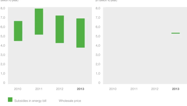
The same conclusion can be drawn by considering the total costs for electricity generation to be paid for by the electricity users. Figure 2.2 shows the wholesale price3_{component and the total}

energy subsidies paid via the energy bill (2013 figures are estimates). The costs were scaled to 100 TWh (order of magnitude of the Dutch consumption) to make them comparable.

Electricity generation cost per 100 TWh - Netherlands (in Billion €/year)

(in Billion €/year)

2010 2011 2012 2013

Electricity generation cost per 100 TWh - Germany

8,0 7,0 6,0 5,0 4,0 3,0 2,0 1,0 0 2010 2011 2012 2013 8,0 7,0 6,0 5,0 4,0 3,0 2,0 1,0 0 Wholesale price

Subsidies in energy bill

Figure 2.2 Electricity generation costs per 100 TWh to be paid for by the electricity users. Source: Berenschot (data: CWE Market Coupling data; Rijksoverheid; BDEW).

The German figure shows the sum of the EEG Umlage generated per year as a result of the volumes of renewable energy and the feed-in tariff. The EEG Umlage for households, as shown before, displays a different pattern; this is explained by the way in which these costs are allocated to the end-consumer bill.

The Dutch figure shows the allocation of part of the SDE+ energy subsidies to the Dutch energy bill, a mechanism put into place in order to finance the increase of subsidies for renewable energy. This was introduced by the Dutch government in 2013 for a total of EUR 100 million. In the coming years this will increase to several billion per year. In the Netherlands in 2013, an additional amount of EUR 800 million of subsidies for the production of renewable energy was financed via the state budget, and not via the energy bill.

3_{Throughout this report, unless stated differently, with ‘wholesale price’ we refer to the hourly day-ahead market clearing price published by the respective}

power exchanges.

(6)

2 3

4 5 6

7 8 9

1 2 3

4 5 6

7 8 9

1

Wholesale price

movements and price drivers

Introduction Prices and costs Interconnector

flows Balancing

Future developments Price volatility Overview and

main findings

Before the introduction of market coupling, prices between countries could

be different even if interconnection capacity was still available. These price

differences were partly caused by inefficient interconnector utilisation.

Market coupling results in significant improvements by maximising the interconnector utilisation: either through 100% convergence (where prices between countries are equal); or through

100% utilisation of available interconnector capacity (when prices between countries are different).

Mechanism

Market coupling is a mechanism that was implemented in several steps by TSOs and power exchanges to contribute to the integration of the European electricity market and to optimise the use of interconnection capacity.

The maximisation of the interconnector utilisation through the market coupling mechanism is

achieved through a joint calculation of all wholesale prices by the co-operating exchanges, utilising the interconnector capacity provided by the TSOs. The exchanges share their order books (all electricity bids and electricity offers by their market participants), after which the wholesale prices and cross-border flows for all hours of the next delivery day are calculated in an integrated way. This calculation takes the maximum values into account as provided by the TSOs on a daily basis, for all the hours of the next delivery day. The TSOs calculate this maximum in a coordinated manner from the physical capacity of the interconnector lines and agreed standards for guaranteeing the secure grid operation. This whole exercise results in a schedule with the right flows in the right directions, allowing the most competitive generators to supply to the market.

Results

Wholesale electricity prices in Europe have experienced significant developments over the past

10 years. Initially, wholesale prices in different countries were independent of each other. This changed drastically following the increase of interconnection capacity and the introduction of market coupling. Firstly, at the end of 2006, Trilateral Market Coupling (TLC) was implemented between the Netherlands, Belgium and France. This was followed by the implementation of Central West European (CWE) Market Coupling at the end of 2010 between these TLC countries, Germany and Luxemburg.

Market coupling

(7)

2 3

4 5 6

7 8 9

1 2 3

4 5 6

7 8 9

1

Wholesale price

flows Balancing

main findings

The converging effect of market coupling is best illustrated by the way the prices in the Netherlands, France and Belgium approached each other after the implementation of TLC at the end of 2006:

Daily average prices for TLC countries (in €/MWh)

120 100 80 60 40 20 0 APX - NL Belpex - BE EPEX - FR

Nov 2006 Dec 2006 Jan 2007 Feb 2007 Mar 2007 Apr 2007

Trilateral market coupling (NL, BE, FR)

Figure 3.1 Trilateral Market Coupling. Source: APX; EPEX.

From 2007, the prices of the Netherlands, Belgium and France converged as a result of Trilateral Market Coupling. In 2008 and 2009, strong upward and downward hikes were observed, in which country prices stayed close together. Since 2009, we have seen an increase in all power prices, still largely converging through the TLC effect and even more as a result of the CWE Market Coupling in 2010. This is further demonstrated by figure 3.2, showing the results for the Dutch-German border before and after implementation of CWE Market Coupling. It shows that after implementation there can only be a price difference when the capacity is fully utilised.

Price difference Germany and the Netherlands (€/MWh)

Interconnector utilisation (in %) vs. price difference (in €/MWh) before and after CWE market coupling. Q4 2010

Utilisation ratio (Flow/ATC) 40 20 0 -20 -40 -60 -80 -100 Pre CWE CWE 0 -100 100 80 60 40 20 -20 -40 -60 -80

Figure 3.2 Price difference between Germany and the Netherlands plotted against the utilisation ratio of the interconnection capacity for the fourth quarter of 2010. Source: TenneT (data: APX; EPEX).

(8)

2 3

4 5 6

7 8 9

1 2 3

4 5 6

7 8 9

1

Wholesale price

flows Balancing

main findings

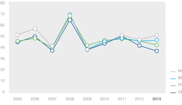
Figure 3.3 shows the prices of the CWE countries France, Belgium, Germany and the Netherlands over the past few years.

Yearly average of Day-Ahead Wholesale Prices in CWE countries(in €/MWh)

80 70 60 50 40 30 20 10 0 2005 2006 2007 2008 2009 2010 2011 2012 2013 NL BE FR DE Figure 3.3 Yearly average of day-ahead wholesale prices in CWE countries. Source: APX; EPEX.

From the end of 2011, prices started to diverge. The average German wholesale price moved downward, while other wholesale prices stayed on the same level, or – in case of the Netherlands – showed an increase. Supported by market coupling, this led to an increase in interconnector utilisation as will be further illustrated in chapter 5 on interconnector flows (see figures 5.1 and 5.2). Price convergence between Germany and the Netherlands (in % of hours)

% Price Convergence % Interconnector Utilisation 100% 90% 80% 70% 60% 50% 40% 30% 20% 10% 0%

January _February March

April May June July

August

September

October

November December January February

March April May June July _August

September

October

September

October

November December

2011 2012 2013

Figure 3.4 Price convergence between Germany and the Netherlands. Source: Berenschot (data: CWE Market Coupling data).

(9)

2 3

4 5 6

7 8 9

1 2 3

4 5 6

7 8 9

1

Wholesale price

flows Balancing

main findings

Figure 3.4 clearly shows that Market Coupling initially resulted in a large price convergence. From the end of 2011, the outcome is less price convergence and more interconnector utilisation, driven by changes discussed in the following chapters. In all cases, market coupling optimises the prices and interconnector flows by allowing competitive generators to benefit optimally from export capacity and by allowing consumers to benefit optimally from import capacities.

Further expansion

On February 4, 2014, the coupling of the North Western European market was successfully implemented by the TSOs and the Power Exchanges now applying the same mechanism of market coupling to 15 countries in North Western Europe4_{. This represents a major step for}

European market integration.

4_{CWE and ITVC market coupling, as well as the APX-operated market coupling for the BritNed interconnector, were replaced by this NWE market coupling.}

(10)

2 3

4 5 6

7 8 9

1 2 3

4 5 6

7 8 9

1

Interconnector

flows

Introduction Prices and costs Market coupling Balancing Future

developments Price volatility Overview and

main findings

The sections below discuss the fundamental drivers of the recent

development of price differences:

• The generation assets

• The development of renewable energy sources

• The development of prices for coal, gas and CO

₂

• Weather-dependent price developments

Generation assets

Typically, the generation base in a country evolves over time and is the reflection of its access to natural resources and political choices.

There has always been a tendency to use indigenous resources, but access to imports due to geographical location near exporting countries or resulting from seaports also plays a big role. These resources can be fossil, but also renewable, such as potential for hydro power, solar energy, biomass and wind speed.

In addition to access to resources, political choices in the past and current energy policy play a major role determining a country’s generation base. Whether or not to deploy nuclear energy, for instance, is one of the main questions on which European countries differ. Comparing the Netherlands and Germany, we see the following picture (figure 4.1).

Wholesale price

movements

and price drivers

Wholesale price movements and price drivers

(11)

2 3

4 5 6

7 8 9

1 2 3

4 5 6

7 8 9

1

Interconnector

flows

main findings

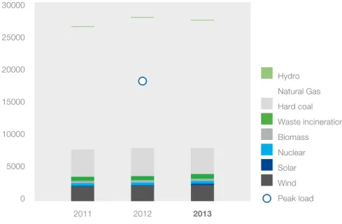
2011 2012 2013

Installed Production Capacity in the Netherlands (in MW)

30000 25000 20000 15000 10000 5000 0 Biomass Nuclear Waste incineration Hard coal Natural Gas Hydro Wind Solar Peak load 2011 2012 2013

Installed Production Capacity in Germany (in MW)

200000 160000 120000 80000 40000 0 Nuclear Peak load Biomass Hard coal Lignite Natural gas Hydro Oil Other Wind Solar Solar

Figure 4.1 Generation capacity in Germany and the Netherlands. Source: TenneT/IAEW Aachen (data TenneT; Bundesnetzagentur (2013 preliminary figures).

As shown in figure 4.1, the electricity generation in the Netherlands is more dependent on gas generation, while Germany has a more varied generation base including lignite, a larger share of nuclear, and more hard coal plants. The share of renewables will be discussed in the following section. The rise in installed capacity in Germany shown in figure 4.1 is not the result of a rise in (peak)

demand but mainly the result of policy-induced investment. As a result, the utilisation rate of the generation base as a whole is bound to decline. As intermittent sources cannot fully replace dispatchable capacity due to its uncertain production, this has consequences for the total costs of the system.

(12)

2 3

4 5 6

7 8 9

1 2 3

4 5 6

7 8 9

1

Interconnector

flows

main findings

Furthermore, it is important to mention that in markets that work based on a clearing price, it is the marginal unit that sets the market price. If, for instance, despite a different generation base in both countries, a gas-fired power plant sets the price, the prices would still be at a similar level. Furthermore, import and export, facilitated by market coupling, could still lead to identical prices in a large number of hours, as was witnessed in 2010.

In the following section we examine price developments that are driven by changes in the generation assets, but also by changes affecting the relative competitiveness of the existing generation assets, with changes in fuel prices as the most important driver. The impact of these changes will vary according to the generation base.

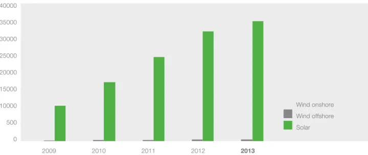
Development of renewable energy sources

Electricity generated from renewable energy sources increasingly contributes to the overall generation mix, especially in Germany. As result of the Renewable Energy Act, which provided a stable policy favouring renewable energy sources, the deployment of these sources has shown spectacular growth over the last couple of years. The development of the installed capacity is shown in figure 4.2.

Installed renewable production capacity in Germany (in MW)

Solar Wind offshore Wind onshore 2010 2009 2011 2012 2013 40000 35000 30000 25000 20000 15000 10000 500 0

Figure 4.2 Development of installed production capacity for wind and solar energy in Germany. Source: IAEW (data: AGEE, BNetzA, 2013: Prognosis as per October 2013).

Despite a growth of installed capacity in Germany, the generation from wind was moderate between 2012 and 2013 due to relatively feeble winds. There was a growth in electricity production from biomass, yet the overall growth of production from renewables was relatively small.

(13)

2 3

4 5 6

7 8 9

1 2 3

4 5 6

7 8 9

1

Interconnector

flows

main findings

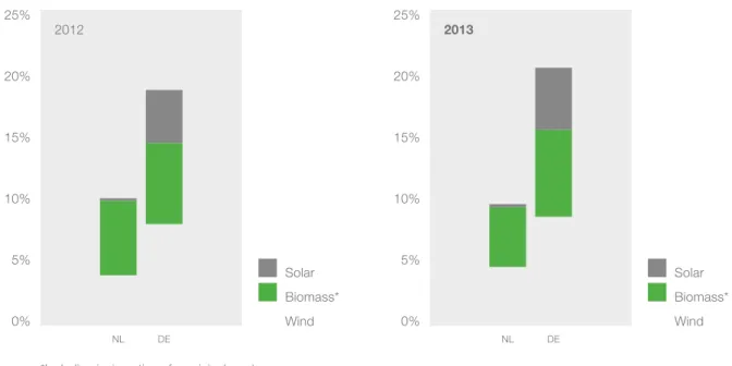
Nevertheless, the development has created a substantial gap between Germany and the Netherlands. Where the contribution of renewable energy to the total electricity consumption in Germany was some 25% in 2013, in the Netherlands this was 10%. Figure 4.3 shows the contribution of wind, solar and biomass as they are the main contributors in Germany and are virtually the only contributors in the Netherlands.

Contribution of renewable energy production to total electricity consumption

25% 20% 15% 10% 5% 0% 2012 2013 NL DE NL DE Wind Biomass* Wind Biomass* Solar Solar 25% 20% 15% 10% 5% 0% *Including incineration of municipal waste

Figure 4.3 Electricity production from wind, solar and biomass divided by the national electricity consumption for Germany and for the Netherlands. Source: Berenschot (data CBS; AGEB).

The difference is substantial for all three sources, but the difference in the contribution of solar is most striking.

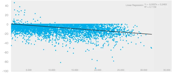
A further analysis of the influence of renewable production on the price difference between Germany and the Netherlands is shown in figure 4.4. In this graph, the production of renewable energy has been plotted against the price difference for each hour.

(14)

2 3

4 5 6

7 8 9

1 2 3

4 5 6

7 8 9

1

Interconnector

flows

main findings

Correlation between price differences and generation from wind and solar for each hour in 2012

Wind and solar production Germany (MW)

Linear Regression: Y = -0,0007x + 0,2463 R2_{= 0,1139}

5.000

40 20 0 -20 -40 -60 -80 -100 10.000 15.000 20.000 25.000 30.000 35.000

Correlation between price differences and generation from wind and solar for each hour in 2013

Wind and solar production Germany (MW)

5.000

40 20 0 -20 -40 -60 -80 -100 10.000 15.000 20.000 25.000 30.000 35.000 Linear Regression: Y = -0,0009x + 6,0865 R2_{= 0,2556}

Figure 4.4 Influence of renewables production in Germany on price difference DE-NL. Source: IAEW Aachen (data: EPEX; APX; EEX Transparency).

(15)

2 3

4 5 6

7 8 9

1 2 3

4 5 6

7 8 9

1

Interconnector

flows

main findings

The analysis shows that renewable energy generation is indeed a driver of the difference in wholesale prices that has been witnessed in these years. However, it also shows that it is not the only driver of this development.

Moreover, it should be noted that realisation of the targets laid down in the Dutch Energy Agreement, which was signed in September 2013, means that the gap between the share of wind energy in the generation capacity in the Netherlands and Germany will be bridged. It is to be expected that this will contribute to price convergence between the Netherlands and Germany (i.e. it will further reduce the correlation shown in figure 4.4).

The section on weather-dependent price developments will discuss the impact of volatile production of intermittent renewables in more detail.

Prices of coal, gas and CO

₂

In 4.1 we saw that the current electricity generation mix is still largely provided by fossil fuel power plants. The prices of fossil fuel-generated electricity are mainly driven by the prices for primary energy and CO₂ emission allowances. These prices are equally valid for the Netherlands and Germany. Although coal prices and gas prices show slight differences between the Netherlands and Germany, these differences are not considered an impediment for general analysis.

The following graphs show the development of the prices of hard coal, natural gas and CO₂ over the past four years.

(16)

2 3

4 5 6

7 8 9

1 2 3

4 5 6

7 8 9

1

Interconnector

flows

main findings

Development of Natural Gas Price 2010-2013 (TTF Spot; in €/MWh)

€ 35 € 30 € 25 € 20 € 15 € 10 € 5 € 0

April May June July

August

September

October

September

October

September

October

September

October

November December

2010 2011 2012 2013

Development of Hard Coal Price 2010-2013 (CIF ARA; in €/ton)

€ 120 € 100 € 80 € 60 € 40 € 20 € 0

April May _June July

August

September

October

September

October

September

October

September

October

November December

2010 2011 2012 2013

Development of EUA Carbon Futures 2010-2013(in €/ton CO2)

€ 18 € 16 € 14 € 12 € 10 € 8 € 6 € 4 € 2 € 0

August

September

October

September

October

September

October

September

October

November December

2010 2011 2012 2013

Figure 4.5. Development of primary energy prices. Source: Berenschot (data ICE ENDEX; Spectron; EEX; Energate).

(17)

2 3

4 5 6

7 8 9

1 2 3

4 5 6

7 8 9

1

Interconnector

flows

main findings

As shown in these figures, hard coal prices and CO₂ prices have come down over the last two years, while gas prices have increased. As the CO₂ price has a higher impact on the coal-fired generation, a lower CO₂ price favours coal. This means that all three developments work in the same direction: improving the competitive position of coal compared to gas.

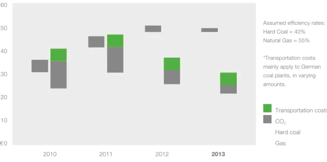
The effect of these market developments on the marginal generation costs of electricity is shown in figure 4.6. Costs of German and Dutch coal plants are calculated on the same basis. For German coal plants, a substantial additional cost factor can apply depending on coal transportation cost; this cost factor is smaller for coal plants that are located nearer seaports (typically the case for the Dutch plants).5

2010 2011 2012 2013

Marginal generation costs of electricity: gas vs. coal (in €/MWh)

€ 60 € 50 € 40 € 30 € 20 € 10 € 0 Gas Hard coal CO2 Transportation costs* Assumed efficiency rates: Hard Coal = 40% Natural Gas = 55% *Transportation costs mainly apply to German coal plants, in varying amounts.

Figure 4.6 Marginal generation costs of electricity. Source: Berenschot/IAEW Aachen (data: APX, TTF Day-Ahead, Energate, Spectron).

Figure 4.6 shows the deteriorating position of gas relative to coal. Despite lower costs for CO₂ emission allowances, the generation costs of gas turbines went up due to higher prices for natural gas. On the basis of falling prices for hard coal combined with those for CO₂, generation costs of hard coal plants fell. As shown, the marginal generation cost of gas- and coal-fired generation were about the same in 2010. Yet from 2011-2013, the gap widened. This has substantially influenced the merit order of power plants in both the Netherlands and Germany. In both countries, the marginal price for coal plants has become much lower than for gas plants.

This has occurred in the same time period as the occurrence of the price gap between these countries. The larger share of hard coal plants discussed in the section 4.1 indicates that the

increasing spread in generation costs between gas and coal is also an explanation of the divergence of wholesale prices between the two countries. As gas-fired generation is more often the marginal unit in the Netherlands, and coal-fired generation more often in Germany, the spread in generation costs between the fuels also translates into a price spread between the countries.

5_{Gas transportation costs (exit fees) are not considered in this exercise as they are not considered to be marginal.}

(18)

2 3

4 5 6

7 8 9

1 2 3

4 5 6

7 8 9

1

Interconnector

flows

main findings

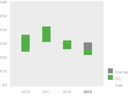
Another reason for the difference in impact lies in the introduction of the coal tax in the Netherlands in 2013. This has affected the generation cost of coal-fired plants in the Netherlands, almost evening

out the favourable developments of reduced coal- and CO₂ prices. This mechanism has reduced

the competitiveness of Dutch coal plants and affected their position in the European merit order.

2010 2011 2012 2013

Marginal coal-fired generation costs including Dutch coal tax (in €/MWh)

CO2 Coal Coal tax € 60 € 50 € 40 € 30 € 20 € 10 € 0

Figure 4.7 Marginal coal-fired generation costs in the Netherlands. Source: Berenschot (tax data Rijksoverheid).

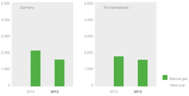
The developments as described above are reflected in the development of the number of full load hours of gas- and coal-fired power plants in the Netherlands and Germany (figure 4.8). In both countries, the operational hours for gas plants have decreased, in Germany more so in 2013 than in the Netherlands. If interconnection capacity is fully utilised and price developments in surrounding countries have no further influence, this will mitigate the effect on gas-fired power plants in

the Netherlands.

(19)

2 3

4 5 6

7 8 9

1 2 3

4 5 6

7 8 9

1

Interconnector

flows

main findings

2012 2013 2012 2013

Full load hours in Germany and the Netherlands (in h/a)

Germany The Netherlands 5.000 4.000 3.000 2.000 1.000 0 Hard coal Natural gas 5.000 4.000 3.000 2.000 1.000 0

Figure 4.8 Full load hours in Germany and the Netherlands. Source: IAEW Aachen/TenneT (data Statistische Bundesamt; EEX). Preliminary figures for 2013.

However, since the relative capacity of gas is much higher in the Netherlands, gas plants are still the marginal plant in the merit order in the Netherlands rather than in Germany. The correlation between the Dutch wholesale electricity price and the market price of natural gas is prominently visible when plotting the monthly development of the marginal generation costs (cost of gas plus cost of CO₂) against the baseload wholesale price (figure 4.9). Also, this correlation is stronger when interconnection capacity is fully utilised.

(20)

2 3

4 5 6

7 8 9

1 2 3

4 5 6

7 8 9

1

Interconnector

flows

main findings

Marginal gas-fired generation costs versus wholesale electricity baseload prices in the Netherlands

€ 70 € 60 € 50 € 40 € 30 € 20 € 10 €

-Marginal gas-fired generation costs (gas + CO2 price based) Wholesale baseload day-ahead price

August

September

October

September

October

September

October

September

October

November December

2010 2011 2012 2013

Figure 4.9 Marginal gas fired generation costs and the monthly average of the day ahead wholesale prices.

Source: Berenschot (data ICE ENDEX; CWE Market Coupling data). Preliminary results for 2013. Emission factor: 56,5 kg/ GJ. Assumed efficiency: 55%.

Weather-dependent price developments

This section concentrates on the differences in wholesale prices in the CWE countries encountered within the year. These intra-year developments are mostly driven by temperature (with a seasonal pattern) and the development of wind speeds (partly seasonal) and solar hours (seasonal and daily). Other possible influences are the precipitation, which can influence the amount of hydropower available in countries such as Norway and Switzerland.

Seasonal patterns

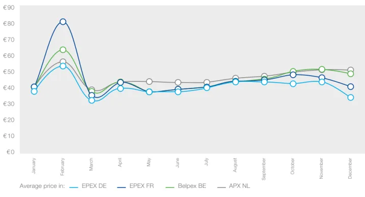
Seasonal variations are visible each year, mostly influenced by cold weather situations. As an example, the variation of CWE wholesale prices over the year is shown in figure 4.10.

(21)

2 3

4 5 6

7 8 9

1 2 3

4 5 6

7 8 9

1

Interconnector

flows

main findings

The year 2012 in more detail: CWE monthly average wholesale prices

€ 90 € 80 € 70 € 60 € 50 € 40 € 30 € 20 € 10 € 0 EPEX DE

Average price in: EPEX FR Belpex BE APX NL

August

September

October

November December

EPEX DE

Average price in: EPEX FR Belpex BE APX NL

The year 2013 in more detail: CWE monthly average wholesale prices

August € 70 € 60 € 50 € 40 € 30 € 20 € 10 € 0

September

October

November December

Figure 4.10 Monthly average wholesale prices in 2012 and 2013. Source: Berenschot (data: CWE Market Coupling data).

The French price shows a substantial increase during cold weather periods, while the Dutch price does not show the same seasonal dependence. This phenomenon is caused by the usage of electric heating in France. The Netherlands does not have such a demand for electric heating; instead, cold weather causes more supply by cogeneration plants. Therefore, the Dutch price varies less over the year.

(22)

2 3

4 5 6

7 8 9

1 2 3

4 5 6

7 8 9

1

Interconnector

flows

main findings

Apart from the above-mentioned influences on the demand side, seasonal effects also play a role on the supply side. Figure 4.10 also shows a decreasing German price during the summer period. This can partly be explained by the monthly input of solar energy, which is illustrated in figure 4.11. Monthly average hourly production of wind and solar in Germany in 2012 (in 1.000 MWh/h)

12 10 8 6 4 2 0 12 10 8 6 4 2 0 November October June September January April August March July February

December October November

June September January April August March July February December 2012 2013 Solar Wind

Figure 4.11 Monthly average hourly production of wind and solar. Source: IAEW Aachen (data: German TSOs).

It is interesting to see that monthly averages vary substantially throughout the year, but also between the years. This is true for wind (compare the October months) but also for solar (compare for instance July).

(23)

2 3

4 5 6

7 8 9

1 2 3

4 5 6

7 8 9

1

Interconnector

flows

main findings

Weekly patterns

Apart from the seasonal and monthly variation, weekly demand patterns can also have an influence on pricing, especially when combined with the input of renewable energy. This is shown in the figure of daily baseload prices in Germany and the Netherlands.

The Year 2013 in daily detail: daily average wholesale prices in Germany and in the Netherlands

01-01-13 08-01-13 15-01-13 22-01-13 29-01-13 05-02-13 12-02-13 19-02-13 26-02-13 05-03-13 12-03-13 19-03-13 26-03-13 02-04-13 09-04-13 16-04-13 23-04-13 30-04-13 07-05-13 14-05-13 21-05-13 28-05-13 04-06-13 11-06-13 18-06-13 25-06-13 02-07-13 09-07-13 16-07-13 23-07-13 30-07-13 06-08-13 13-08-13 20-08-13 27-08-13 03-09-13 10-09-13 17-09-13 24-09-13 01-10-13 08-10-13 15-10-13 22-10-13 29-10-13 05-11-13 12-11-13 19-11-13 26-11-13 03-12-13 10-12-13 17-12-13 24-12-13 31-12-13 € 80 € 70 € 60 € 50 € 40 € 30 € 20 € 10 € 0 -€ 10 EPEX DE APX NL

Figure 4.12 Daily prices in Germany and the Netherlands. Source: Berenschot (data: CWE Market Coupling data).

This figure contains three main messages: firstly, the price in Germany is lower than in the Netherlands (already discussed above); secondly, the price in Germany shows stronger variation (discussed in chapter 6 ‘volatility’); thirdly, there is a strong weekly pattern (discussed below).

The weekly pattern of price dips in weekend days can be observed for both countries, but this is much more prominent for Germany. Looking at the average weekly pattern shown below (figure 4.13), we can confirm that the average price difference between the Netherlands and Germany at weekends is indeed larger than on weekdays.

(24)

2 3

4 5 6

7 8 9

1 2 3

4 5 6

7 8 9

1

Interconnector

flows

main findings

Hourly average wholesale price on weekdays (Mon-Fri) in Germany and in the Netherlands in 2013 (in €/MWh)

70 60 50 40 30 20 10 0

Hourly average Netherlands Hourly average Germany

1 2 3 4 5 6 7 8 9 10 11 12 13 14 15 16 17 18 19 20 21 22 23 24

Hourly average wholesale price on weekend (Sat-Sun) in Germany and in the Netherlands in 2013 (in €/MWh)

70 60 50 40 30 20 10 0

Hourly average Netherlands Hourly average Germany

1 2 3 4 5 6 7 8 9 10 11 12 13 14 15 16 17 18 19 20 21 22 23 24

Figure 4.13 Hourly average wholesale price on weekdays and weekend days. Source: Berenschot/IAEW Aachen (data: CWE Market Coupling data, EPEX, APX, German TSOs).

On average, prices on weekend days are around 10 €/MWh lower than prices on Monday to Friday. Moreover, it can be observed that German prices are constantly levelling below Dutch market prices. However, the price difference between the countries during weekdays is significantly lower, with an average of 12 €/MWh compared to 19 €/MWh on weekend days.

(25)

2 3

4 5 6

7 8 9

1 2 3

4 5 6

7 8 9

1

Interconnector

flows

main findings

The effective electricity demand to be covered by German power plants can be quite low during weekend conditions, resulting from a low demand combined with high inputs of renewable energy. This will push the market clearing price further down the merit order. In Germany, during weekend days, even hard coal plants are often out of the money. In these hours, the lowest-cost plants set the price, such as nuclear, lignite and must-run-CHP, or even renewables.

Due to the already high utilisation of the Dutch-German interconnectors, the Netherlands cannot benefit from this further price decrease in Germany, which is reflected in persistently higher Dutch prices on weekend days. This is also visible at night-time, as prices in the Netherlands will still be set by coal- or even gas-fired generation.

Daily patterns

Electricity demand sees a daily pattern based on the hourly variations in demand, following more or less a day-night pattern. This general pattern of low prices at night and a morning and an evening peak can be observed in all CWE countries, as can be seen in figure 4.14.

Hourly average wholesale price on Tuesdays in 2013 in CWE Countries (in €/MWh)

70 60 50 40 30 20 10 0 NL FR DE BE 1 2 3 4 5 6 7 8 9 10 11 12 13 14 15 16 17 18 19 20 21 22 23 24

Figure 4.14 Daily price curve on an average Tuesday. Source: Berenschot (data: CWE Market Coupling data).

(26)

2 3

4 5 6

7 8 9

1 2 3

4 5 6

7 8 9

1

Interconnector

flows

main findings

Closer observation shows that the price difference between Germany and the other countries is greater between the peaks (between 9h00 and 17h00). This time period coincides with the production of electricity from solar energy. The daily pattern of solar is shown in figure 4.15.

Hourly average wholesale price in 2013 (in €/MWh)

70 60 50 40 30 20 10 0 DE NL NL - DE 1 2 3 4 5 6 7 8 9 10 11 12 13 14 15 16 17 18 19 20 21 22 23 24

German average hourly solar production for days in 2013 (in MWh/h)

12.500 10.000 7.500 5.000 2.500 0 1 2 3 4 5 6 7 8 9 10 11 12 13 14 15 16 17 18 19 20 21 22 23 24

Figure 4.15 Price differences compared to solar input. Source: IAEW Aachen (data: EPEX, APX and EEX Transparency).

(27)

2 3

4 5 6

7 8 9

1 2 3

4 5 6

7 8 9

1

Interconnector

flows

main findings

Hourly differences and wind and solar energy

The analysis in the preceding sections describes developments based on averages. The true concern when it comes to intermittent sources are the variations contained in these averages. In the picture below we see the variation over a week in Germany in 2012. In this week, a combination of high wind and solar input on a Sunday, with typical low demand, pushes wholesale prices to negative values. In such situations, all flexible conventional generation that actively participates in the market will be switched off. Although most wind farms have the technical means to be switched off, the subsidy schemes often do not incentivise this.

Monday Tuesday Tuesday Wednesday Thursday Friday Saturday Sunday

Variation of consumption and production over an exemplary week in Germany

80.000 70.000 60.000 50.000 40.000 30.000 20.000 10.000 0 -10.000 80 70 60 50 40 30 20 10 0 -10

Solar Wind Residual Consumption Consumption Wholesale Price (in €/MWh/h)

MWh/h €/MWh

Figure 4.16 Infeed from solar and wind compared to consumption. Source: IAEW Aachen (German TSOs; EPEX).

Moreover, high gradients of the residual load of up to 9 GW/h and of the wholesale prices with

a difference of more than 15 €/MWh within two adjacent hours. The load gradients and resulting price differences reflect the challenges for the grid and the remaining generation stack in these situations to provide the flexibility needed. Additionally, the importance of load, wind and solar prognosis of high quality becomes obvious in order to forecast such situations.

(28)

2 3

4 5 6

7 8 9

1 2 3

4 5 6

7 8 9

1

Price volatility

Introduction Prices and costs Market coupling

Wholesale price movements and price drivers Balancing Future developments Overview and main findings

The utilisation rate of interconnectors is influenced by several (changeable)

factors, of which generation base, fuel prices, energy policies and weather

patterns are considered most important in the period analysed in this Market

Review. To go into further detail, the following chapter describes the changes

in interconnector flows

6

_{between 2012 and 2013 for all CWE country borders.}

Border Germany – Netherlands

Figure 5.1 shows the border flows between Germany and the Netherlands compared to Net Transfer Capacity. It appears that the flow from Germany to the Netherlands has increased significantly, which is consistent with the higher average price difference between these countries in 2013.

DE > NL NL > DE

Volume at 100% utilisation

Germany - Netherlands Amount of nominated border flows (in TWh)

30 25 20 15 10 5 0 -5 -10 -15 -20 -25 -30 30 25 20 15 10 5 0 -5 -10 -15 -20 -25 -30 20 17,1 -20,3 2012 2013 19,5 _18,5 -0,2 -20,1 -0,6

Figure 5.1 Border flows Germany - Netherlands. Source: Berenschot (data: CWE Market Coupling data).

Interconnector

flows

6_{Throughout this report we did not consider the results from cross border intraday transactions on the utilisation of the interconnectors.}

The flows reflect the commercial flows resulting from nominations on capacity from long term auctions (annual and monthly capacity) and the outcome of day-ahead market coupling.

Interconnector flows

(29)

2 3

4 5 6

7 8 9

1 2 3

4 5 6

7 8 9

1

Price volatility

The growing shift in utilisation of crossborder capacity, mostly in the German-Dutch direction, previously mentioned in relation to figure 3.4, is shown by figure 5.2. Here percentages are shown relative to Available Transfer Capacity (ATC) for this market coupling7_{. As illustrated, the outcome of market}

coupling on the German-Dutch border has shifted substantially from 100% price convergence for most situations towards a situation with price differences and a higher, almost 100% interconnector utilisation. Volume % utilisation NL > DE (2011-2013)(in time %)

100% 90% 80% 70% 60% 50% 40% 30% 20% 10% 0%

August

September

October

September

October

September

October

November December

2011 2012 2013

Volume % utilisation DE > NL (2011-2013)(in time %)

100% 90% 80% 70% 60% 50% 40% 30% 20% 10% 0%

August

September

October

September

October

September

October

November December

2011 2012 2013

Figure 5.2 Percentage of interconnector utilisation Germany - Netherlands. Source: Berenschot (data: CWE Market Coupling data).

7_{This ATC does not include the long-term capacity scheduled by market parties ahead of the day-ahead market coupling calculation.}

(30)

2 3

4 5 6

7 8 9

1 2 3

4 5 6

7 8 9

1

Price volatility

Looking at the directions more specifically, we see that flows from the Netherlands to Germany still occurred substantially in 2011, but no longer, or only incidentally, in 2012 and 2013. In contrast, flows from Germany to the Netherlands have strongly increased, which is in line with the overall development.

Border Netherlands - Belgium

Generally, the situation on the Dutch-Belgian border is different from the Dutch-German border. The Dutch and Belgian markets are often coupled with flows in both directions, whereby the direction is determined by price equilibrium calculation. Contingent differences in Belgian and Dutch prices occur in either direction, meaning that the Belgian price is higher for some hours, while the Dutch price is higher for other hours. Contrary to developments on the German-Dutch border, patterns on the Belgian-Dutch border have stayed more or less the same in 2013 compared to 2012, as shown below.

Belgium - Netherlands Amount of nominated border flows (in TWh)

15 10 5 0 -5 -10 -15 11,4 5,6 -2,7 -11,8 BE > NL NL > BE Volume at 100% utilisation 15 10 5 0 -5 -10 -15 11,9 5,9 -2,9 -11,8 2012 2013

Figure 5.3 Border flows Belgium - Netherlands. Source: Berenschot (data: CWE Market Coupling data).

On a yearly average, the majority of flows occur from Belgium to the Netherlands. However, large monthly variations are noticeable, as shown in the monthly graphs for flows in both directions in figure 5.4.

(31)

2 3

4 5 6

7 8 9

1 2 3

4 5 6

7 8 9

1

Price volatility

Volume % utilisation BE > NL (2011-2013)(in volume %)

100% 90% 80% 70% 60% 50% 40% 30% 20% 10% 0%

April May June July

August

September October November December

April May June July

August

April May June July

August

2011 2012 2013

Volume % utilisation NL > BE (2011-2013)(in volume %)

100% 90% 80% 70% 60% 50% 40% 30% 20% 10% 0%

April May June July

August

April May June July

August

April May June July

August

2011 2012 2013

Figure 5.4 Percentage of interconnector utilisation. Source: Berenschot (data: CWE Market Coupling data).

This monthly pattern repeats on a yearly basis, suggesting a seasonal pattern whereby the flow in the winter tends to be in the direction of Belgium, while the flow in summer tends to be in the direction of the Netherlands. This is indeed consistent with monthly price developments for 2012 and 2013.

(32)

2 3

4 5 6

7 8 9

1 2 3

4 5 6

7 8 9

1

Price volatility

As seen before, French and Belgian prices can rise above Dutch prices in cold winter periods. This is caused by the higher demand for electrical heating in France. As the Belgian market is coupled to the French market, the Belgian market follows the French price movements to some extent.

In addition, the Belgian market experienced a shortage in the first 5 months of 2013, due to an extended outage of nuclear power plants. As a result, during that period, the Belgian price remained coupled with the Dutch price, as can be seen in the monthly price development in figure 4.10.

Border Belgium - France

The Belgian-French border shows flows mostly from France to Belgium, yet there are situations in which the flow reverses (for instance in cold winter periods as explained above). Given this pattern, there is little difference between 2012 and 2013 (figure 5.5).

2012 2013

Belgium - France Amount of nominated border flows (in TWh)

14,5 1,3 -12,9 -25,5 BE > FR FR > BE Volume at 100% utilisation 12,8 0,8 -10,7 -22,7 30 25 20 15 10 5 0 -5 -10 -15 -20 -25 -30 30 25 20 15 10 5 0 -5 -10 -15 -20 -25 -30

Figure 5.5 Border flows Belgium - France. Source: Berenschot (data: CWE Market Coupling data).

Border Germany - France

Border flows between Germany and France can be noted in both directions. It is only in the summer months (June, July or August) that the flows mainly go from France to Germany. In contrary, in cold winter periods the opposite flows occur caused by the French temperature-dependent electrical heating demand. The yearly utilisation of the Net Transfer Capacities (NTC) between Germany and France can be seen in the following figure 5.6.

(33)

2 3

4 5 6

7 8 9

1 2 3

4 5 6

7 8 9

1

Price volatility

Wholesale price movements and price drivers Balancing Future developments Overview and main findings FR > DE DE > FR Volume at 100% utilisation

France - Germany Amount of nominated border flows (in TWh)

30 25 20 15 10 5 0 -5 -10 -15 -20 -25 -30 30 25 20 15 10 5 0 -5 -10 -15 -20 -25 -30 15,8 2,5 -11,3 -22,9 15,7 1,7 -9,7 -22,5 2012 2013

Figure 5.6 Border flows France - Germany. Source: Berenschot (data: CWE market Coupling data).

Grid restrictions lead to asymmetric capacities in both directions. As the capacity on the interconnecting transmission lines is high compared to other transfer capacities, and persistent imbalances are not given, the utilisation is not exhausted. The predominant allocated flow is from Germany to France, although the French power generation system consists largely of nuclear power stations with low marginal generation costs. This picture is persistent for the years 2012 and 2013 and shows no significant changes, neither in the maximum interconnection capacity nor in the overall flows and flow direction.

Due to the German feed-in of solar panels and wind turbines with negligible marginal costs, higher average prices occur in France. Hence, the total allocated border flow from France is just 2.5 TWh/a in 2012 and 1.7 TWh/a in 2013.

(34)

2 3

4 5 6

7 8 9

1 2 3

4 5 6

7 8 9

1

Price volatility

Border Netherlands - Norway (NorNed interconnector)

Generally, the NorNed interconnector is dominated by the differences resulting from the difference in generation mix: hydro in Norway and fossil fuels in the Netherlands. This gives rise to four different possible price-influencing patterns:

1. Changes in fuel prices in the Netherlands and the changes in Norway driven by rainfall and the consequences for water storage in Norway dominate the fundamental price differential. 2. Prices in Norway are more stable during the 24 hours of the day as the price is driven by the

opportunity cost of the water in storage. This can cause NorNed flows to swing in a day-night pattern, which was often experienced in 2009-2011.

3. Seasonal and precipitation patterns. Rainfall and melting snow influence the level of water stored behind dams, which can affect prices in Norway especially in winter situations. Additionally, rainfall can have a direct impact on the production of run-of-river hydro, influencing the prices. The NorNed flow reacts accordingly, for instance by exporting to Norway at times of scarcity. 4. Incidental CWE volatility impact. For instance, at times of high renewable input in Germany, the

German price pushes the Dutch price down as well, causing NorNed flows to export to Norway. The net effect is a storage of German and Dutch renewables into Norwegian hydropower.

In 2012 and 2013, the daily, seasonal and hydro-patterns were not determinative. The main factor driving the flows was an almost permanent large difference between the higher price in the

Netherlands and a much lower average price in Norway, causing a large flow from Norway to the Netherlands in 2012 and 2013 (figure 5.7). Incidentally, there were hours when the opposite was the case, for instance at times of incidental low prices in the Netherlands influenced by low prices in Germany. This limits the Dutch price volatility, as the NorNed interconnector reverses in such cases, mitigating the downward price movements in the Netherlands.

NO > NL NL > NO Volume at 100% utilisation 10 8 6 4 2 0 -2 -4 -6 -8 -10 10 8 6 4 2 0 -2 -4 -6 -8 -10 5,9 _5,7 -5,9

Norway - Netherlands Amount of nominated border flows (in TWh)

5

4,2

-5,1

-0,1 -0,2

2012 2013

Figure 5.7 Border flows Netherlands - Norway. Source: Berenschot (data TenneT).

(35)

2 3

4 5 6

7 8 9

1 2 3

4 5 6

7 8 9

1

Price volatility

Border Netherlands - United Kingdom

The BritNed interconnector shows a situation that is practically the reverse of NorNed in recent years. Due to higher prices in the United Kingdom, the flows have been predominant from the Netherlands to the UK, as is seen both in 2012 and 2013 (figure 5.8). Hours where the opposite was the case have occurred incidentally, for instance at times of incidental high prices in the Netherlands. This limits the Dutch price volatility, as the BritNed interconnector can reverse in such cases, mitigating the upward price movements in the Netherlands.

2012 2013

Netherlands - United Kingdom Amount of nominated border flows (in TWh)

10 8 6 4 2 0 -2 -4 -6 -8 -10 10 8 6 4 2 0 -2 -4 -6 -8 -10 8,6 6,8 -0,3 -8,6 8,7 6,3 -0,3 -8,7 NL > UK UK > NL Volume at 100% utilisation

Figure 5.8 Border flows Netherlands – United Kingdom. Source: Berenschot (data TenneT).

In essence, with the current relative weight of the economic drivers in the electricity market, the Netherlands functions as a hub for the surrounding countries: importing from Germany and Norway and exporting to the United Kingdom.

(36)

2 3

4 5 6

7 8 9

1 2 3

4 5 6

7 8 9

1

Balancing

Wholesale price movements and price drivers Interconnector flows Future developments Overview and main findings

Low volatility of baseload prices over the course of the years is usually

regarded as positive since stable price levels reduce the risks for both

producers and consumers. On the other hand, price volatility as a result

of fluctuating demand within a time period is considered to be a crucial

characteristic of a well-functioning market. High prices during incidental

demand peaks contribute to ensuring sufficient generation capacity.

Price volatility is a measure of the variations of electricity prices over time. It can be measured in standard deviation, reflecting the degree of deviation of any individual price compared to the average price. The lower the standard deviation, the more stable the price. a large standard deviation

corresponds with high price fluctuations.

Previously we saw the volatile pattern of the daily prices for the Netherlands and Germany in figure 4.12. In figure 6.1 this data has been represented as an average combined with a standard deviation. Furthermore, the numbers for France and Belgium are included.

Volatility of daily average wholesale price of CWE Countries in 2013(in €/MWh)

€ 60 € 50 € 40 € 30 € 20 € 10 € 0 BE DE FR NL Average price Figure 6.1 Volatility of electricity prices in 2013 in CWE countries. Source: Berenschot (data: CWE Market Coupling data).

It appears that the volatility of Dutch electricity is lowest of all surrounding countries. Although the Dutch average price is above neighbouring countries, peak prices of other countries can be just as high as peak prices in the Dutch market, or even substantially higher. The same development can be noted when looking at individual hourly market prices.

Price volatility

(37)

2 3

4 5 6

7 8 9

1 2 3

4 5 6

7 8 9

1

Balancing

The causes of the differences in price volatility are country-specific:

• Volatility in the French market is mainly caused by cold-induced demand from electrical heating, as discussed earlier.

• Volatility of Belgian prices has mixed causes. One cause is that the Belgian price frequently alternates between the Dutch price and the French price. Moreover, Belgium is impacted by y volatility

influences from France. Finally, the outage of Belgian nuclear was a factor of volatility in 2013. • Volatility of German prices is often associated with the variations from renewable energy

(wind and solar). Another cause is electrical heating, although less than in France.

• Despite the large amount of renewables, German volatility is lower than, for instance, French. • The volatility of the Dutch price is moderate for several reasons. With a low level of renewables and

very little electrical heating, the Netherlands lacks the volatility factors of other countries. Secondly, there is the stabilising function of CHP, including many small-scale units connected to the wholesale market through aggregators. Thirdly, the Dutch market is stabilised by interconnectors and market coupling to four independent markets: Germany, Belgium and France, UK (BritNed interconnector) and Norway (NorNed interconnector).

The development of volatility over time

Some of the factors stabilising the Dutch wholesale price have been introduced in a series of implementations, as can be illustrated in the development of volatility since 2006. It appears that volatility has since steadily decreased.

Development of volatility of daily average wholesale price in the Netherlands(in €/MWh)

€ 90 € 80 € 70 € 60 € 50 € 40 € 30 € 20 € 10 € 0 2006 2007 2008 2009 2010 2011 2012 2013 Average price Figure 6.2 Volatility of electricity prices in the Netherlands over the years. Source: Berenschot

(data: CWE Market Coupling data).

(38)

2 3

4 5 6

7 8 9

1 2 3

4 5 6

7 8 9

1

Balancing

Daily price swings

The previous graph showed the volatility of daily baseload price. Another interesting angle of looking at volatility is to consider price changes over the course of the day.

The ‘daily spread’, here defined as the difference between the highest and the lowest price on a calendar day, can be taken as an indicator for the volatility over the day. By calculating this daily spread for each day in 2012 and 2013, the following graph can be created showing the number of days per 5€-interval.

Daily spread in 2012

Difference between highest and lowest price on a calender day (in €/MWh, €5 intervals)

Number of days per interval

90 80 70 60 50 40 30 20 10 0 DE NL 0 - 5 _{5 - 10} 10 - 15 15 - 20 20 - 25 25 - 30 30 - 35 35 - 40 40 - 45 45 - 50 50 - 55 55 - 60 60 - 65 65 - 70 70 - 75 75 - 80 80 - 85 85 - 90 90 - 95 _{95 - 100} >100 Daily spread in 2013

Difference between highest and lowest price on a calender day (in €/MWh, €5 intervals)

90 80 70 60 50 40 30 20 10 0 DE NL 0 - 5 _{5 - 10} 10 - 15 15 - 20 20 - 25 25 - 30 30 - 35 35 - 40 40 - 45 45 - 50 50 - 55 55 - 60 60 - 65 65 - 70 70 - 75 75 - 80 80 - 85 85 - 90 90 - 95 _{95 - 100} >100

Figure 6.3 Daily spread. Source: TenneT (data: CWE Market Coupling data).

(39)

2 3

4 5 6

7 8 9

1 2 3

4 5 6

7 8 9

1

Balancing

Difference between highest and lowest price on a calender day (in €/MWh, €5 intervals) Daily spread in 2012

90 80 70 60 50 40 30 20 10 0 FR BE 0 - 5 _{5 - 10} 10 - 15 15 - 20 20 - 25 25 - 30 30 - 35 35 - 40 40 - 45 45 - 50 50 - 55 55 - 60 60 - 65 65 - 70 70 - 75 75 - 80 80 - 85 85 - 90 90 - 95 _{95 - 100} >100

Difference between highest and lowest price on a calender day (in €/MWh, €5 intervals) Daily spread in 2013

90 80 70 60 50 40 30 20 10 0 FR BE 0 - 5 _{5 - 10} 10 - 15 15 - 20 20 - 25 25 - 30 30 - 35 35 - 40 40 - 45 45 - 50 50 - 55 55 - 60 60 - 65 65 - 70 70 - 75 75 - 80 80 - 85 85 - 90 90 - 95 _{95 - 100} >100

Figure 6.3 Daily spread. Source: TenneT (data: CWE Market Coupling data).

Comparing the daily spread between the Netherlands and Germany, it is interesting to observe that the spread is larger in the Netherlands than in Germany for most days. This means that, although the baseload price volatility discussed earlier is lower in the Netherlands, the daily profile is more pronounced. This indicates that the fluctuating production of wind and solar in Germany does not translate into higher fluctuation in hourly prices on normal days.

The distribution of daily spreads in Belgium and France is comparable and shows a shift towards higher values on normal days between 2012 and 2013.

(40)

2 3

4 5 6

7 8 9

1 2 3

4 5 6

7 8 9

1

Balancing

This daily spread could be the driver for investment in storage or demand response. Although there seems to be an interest in the market to explore these possibilities, the current levels of price volatility give little incentive for market parties to invest. The relatively small changes between 2012 and 2013 are not expected to alter this.