Quality Assessment of Exon and Gene Arrays

(1)

Revision Version: 1.1

Quality Assessment of Exon and Gene Arrays

I. Introduction

In this white paper we describe some quality assessment procedures that are computed from CEL files from Whole Transcript (WT) based arrays such as the Human Exon 1.0 ST Array and the Human Gene 1.0 ST Array. Some of the methods detailed here are described in Chapter 3 of the Bioconductor monograph (Gentleman et. al. 2005).

Many of the quality assessment procedures considered here entail computing summary statistics for each array in a set of arrays and then comparing the level of the summary statistics across the arrays. Therefore it is assumed that the user has a set of arrays that would normally be analyzed together to address

substantive biological questions.

The quality assessment procedures discussed in this this white paper focus on using various metrics to identify outlier arrays within the data set. These metrics can identify outliers; however it is impossible to provide hard and fast rules (specific thresholds) as to which arrays to flag as outliers. Such rules need to be developed in the context of particular applications with specific types of samples, combined with balancing the cost of repeating experiments and the cost of drawing wrong conclusions.

II. Quality Assessment Software

This white paper focuses on quality assessment metrics and graphs available through the Expression Console™ software(EC) which is freely available from

http://www.affymetrix.com. EC supports probe set summarization, calculation of various quality assessment metrics, and CHP file generation. EC also supports a variety of visualization and graphing tools to facilitate data quality assessment. EC replaces the previously supported Exon Array Computational Tool (ExACT). It should also be noted that the probe set summarization methods available in EC are implemented in the Affymetrix Power Tools (APT). APT also has the option to calculate the same quality control metrics, however it does not provide any visualization tools. Source code and binaries for multiple platforms are provided for APT.

EC writes the computed quality assessment metrics to the CHP file headers. This enables EC and GeneChip Compatible Software programs to access and

visualize these metrics. The current version of APT does not write the quality assessment metrics to the CHP file header, rather it writes the metrics to a report file. Thus APT generated CHP files lack these metrics in the CHP headers and EC and the other software applications can not visualize them when reading APT generated CHP files.

(2)

When analyzing array data in EC or APT, it is important to note that the specific metrics reported are dependent on both the particular content on the array analyzed (ie “core” versus “full” for exon arrays) and on the algorithm used (ie PLIER vs RMA). Some metrics may not be reported because of the particular algorithm used or because the probesets from which the metric was based were not included in the analysis. For example, the median absolute deviation of residuals is only reported when a model based probeset summarization method is used (e.g., RMA or PLIER).

See the manuals and documentation associated with EC and APT for more information on using these applications and for a more complete listing of metrics reported by these two software applications.

III. Quality Assessment Metrics

A variety of quality assessment metrics are calculated by EC during probeset summarization. The first step is to load up CEL files into an EC study and do a multi-chip analysis of the CEL files. In EC select the probeset summarization method of choice under the analysis menu. For example to run an gene level core analysis on Exon Arrays select Analysis-> Gene Level –> Core:

Sketch or for the gene array select Analysis->Gene Level – Default: RMA-Sketch. Once the analysis is complete, a number of metrics can be visualized

by selecting Graph -> Line Graph – Report Metrics from the menu. The

numeric values of these metrics are can be visualized in EC by selecting

Report-> View Full Report from the menu. (See the EC manual for more information on

using the report and graph features.)

III.A. Probe Level Metrics

The first set of quality assessment metrics are based on probe level data. They are described in detail below.

pm_mean is the mean of the raw intensity for all of the PM probes on the array

prior to any intensity transformations (e.g., quantile normalization, RMA style background correction, etc.). The value of this field can be used to ascertain whether certain chips are unusually dim or bright. Dim or bright chips are not a problem per se, but they warrant a closer inspection of the probeset based metrics to see if a problem results (e.g., unusually high median absolute deviation of residuals, unusually high mean absolute relative log expression values when looking within replicates, etc.). In addition, the pm_mean and bgrd_mean are usually correlated; therefore, a low pm_mean value with a relatively high bgrd_mean value may be indicative of poor data for a sample.

bgrd_mean is the mean of the raw intensity for the probes used to calculate

background prior to any intensity transformations (e.g., quantile normalization, RMA style background correction, etc.). These probes are listed in the BGP file. Note that the bgrd_mean may be higher than the pm_mean. This is because the distribution of GC composition between the background probes and the perfect

(3)

match probes can be very different. For example, on the exon arrays for any given sample there may be no real target for many of the probes. Thus the pm_mean may be very low (at or near background). In contrast the bgrd_mean may be skewed toward higher values due to the GC rich probes present for the high GC count background bins.1

For more information on the background probes and the GC bin based background correction see the “Exon Array Background Correction” white paper.

III.B. Probeset Summarization Based Metrics

The next set of metrics is based on the probe set summarization results. The majority of these metrics are available for different groupings of probesets identified with leading “X_” in the name (e.g., “bac spike” is the hybridization controls). The probeset categories described section IV, Probeset Categories. For those metrics based on a mean, the standard deviation is also reported.

pos_vs_neg_auc is the area under the curve (AUC) for a receiver operating

characteristic (ROC) plot comparing signal values for the positive controls to the negative controls. (See Section IV below for more information on the positive and negative probeset categories). The ROC curve is generated by evaluating how well the probe set signals separate the positive controls from the negative controls with the assumption that the negative controls are a measure of false positives and the positive controls are a measure of true positives. An AUC of 1 reflects perfect separation whereas as an AUC value of 0.5 would reflect no separation. Note that the AUC of the ROC curve is equivalent to a rank sum statistic used to test for differences in the center of two distributions. In the case of the exon and gene arrays the positive and negative controls are pseudo

positives and negatives (see below). In practice the expected value for this metric is tissue type specific and may be sensitive to the quality of the RNA sample. Values between 0.80 and 0.90 are typical. For exon level analysis an additional ROC AUC metric is reported based on Detected Above BackGround (DABG) detection p-values, dabg_pos_vs_neg_auc.

X_probesets is the number of probesets analyzed from category “X”. This can

be useful in identifying those metrics based on a very limited number of probesets (e.g., bacterial spikes) versus those based on a large number of probesets (e.g.,all or positive controls).

X_atoms is the number of probe pairs (in practice the number of perfect match

probes) analyzed from category “X”.

X_mean is the mean signal value for all the probe sets analyzed from category

“X”.

1

Currently the bgrd_mean is only reported for an exon level analysis on the exon array or for gene level analysis using a custom configuration which specifies pm-gcbg. Future versions of EC may report this value for all analysis runs. In APT, this value is reported whenever a BGP file is

(4)

X_mad_residual_mean is the mean of the absolute deviation of the residuals

from the median. As with the others, this is for all probesets analyzed from category “X”. Different probes (features on the chip) will return different intensities when hybridized to a common target. To account for these relative differences in intensity the RMA and PLIER algorithms create models for individual feature responses. One can then use these models to identify chips that have a large number of probes that are behaving differently than predicted by the model, and thus may be indicative of a problematic chip. The difference between the actual value and the predicted value is called the residual. The idea is if there is a robust probe model any given probe will have a typical residual associated with it for this metric (the median residual for that probe is used). If the residual for that probe on any given chip is very different from the median, it means that there is a poorer fit to the model. So, calculating the mean of the absolute value of all the deviations produces a measure of how well or poor all of the probes on a given chip fit the model. An unusually high mean absolute deviation of the residuals from the median suggests problematic data for that chip.

X_rle_mean is the mean absolute relative log expression (RLE) for all the

probesets analyzed from category “X”. This metric is generated by taking the signal estimate for a given probeset on a given chip and calculating the

difference in log base 2 from the median signal value of that probeset over all the chips. The mean is then computed from the absolute RLE for all the probe sets analyzed from category “X”. When just the replicates are analyzed together (e.g., RMA-Sketch on just the replicates from tissue A) the mean absolute RLE should be consistently low, reflecting the low biological variability of the replicates.

III.C. Probeset Signals as Quality Metrics

The last set of quality assessment metrics are individual probeset signal values for various controls. On the gene and exon arrays these include the bacterial spike and polyA spike probesets. These probesets are automatically extracted from the CHP file and included in the CHP headers by EC. This makes it easy to graph and report these probesets. Within EC, any probeset can be graphed by selecting Graph-> Probeset list from the menu. (See the EC manual for more details.)

The main use in looking at specific probeset values is to determine if expected behaviors (i.e., constant expression levels for housekeeping genes, rank order of signal values between spike probe sets) for these probesets are observed. See the probeset category section below for more information on the bacterial and polyA spike control probesets.

IV. Probeset Categories

For many of the quality assessment metrics, values are reported not just for all the probe sets analyzed, but also for particular subsets of probesets. This can be useful when troubleshooting a poorer performing sample as noted below.

(5)

all_probeset is all the probe sets analyzed. The quality metrics reported for this

category are going to be driven by the main source of content in that particular analysis run. For example, an exon level analysis using the “full” content for an exon array will mostly contain results from the exon level probesets against the more speculative parts of the genome. There will be various control probesets and exon level probesets from the known part of the genome of course, but they will make a minor contribution to the metrics in this category. In most cases, this category is the bulk of probesets that will be carried into downstream statistical analysis. Thus the metrics reported for this category will be the most

representative of the quality of the data being used downstream. For users of the Exon array doing speculative exon-level analysis we would recommend doing a separate QC run using the core metaprobeset file to restrict QC metrics to be driven by probesets that are more likely to show expression. If this is not done then an alternative is to use the QC metrics for the pos_control rather than the all_probesets.

bac_spike is the set of probesets which hybridize to the pre-labeled bacterial

spike controls (BioB, BioC, BioD, and Cre). This category is useful in identifying problems with the hybridization and/or chip. Metrics in this category will have more variability than other categories (i.e., positive controls, all probesets) due to the limited number of spikes and probesets for this category.

polya_spike is the set of polyadenylated RNA spikes (Lys, Phe, Thr, and Dap).

This category is useful in identifying problems with the target prep. Metrics in this category will have more variability than other categories (i.e., positive controls, all probesets) due to the limited number of spikes and probesets for this category.

neg_control is the set of putative intron based probe sets from putative

housekeeping genes. Specifically, a number of species specific probesets on 3’ IVT arrays were shown to have constitutive expression over a large number of samples. The genes for these probesets were identified and multiple four probe probesets were selected against the putative intronic regions. (See the

respective exon array design Technote for more information.) Thus in any given sample some (or many) of these putative intronic regions may be transcribed and retained. Furthermore, some (or many) of the genes may not be constitutive within certain data sets. These caveats aside, this collection makes for a moderately large collection of probesets which in general have very low signal values. These probesets are used to estimate the false positive rate for the pos_vs_neg_auc metric.

pos_control is the set of putative exon based probe sets from putative

housekeeping genes. Specifically, a number of species specific probesets on 3’ IVT arrays were shown to have constitutive expression over a large number of samples. The genes for these probesets were identified and multiples of four probe probesets were selected against the putative exonic regions. (See the respective exon array design Technote for more information.) Thus in any given sample some (or many) of these putative exonic regions may not be transcribed or may be spliced out. Furthermore, some (or many) of the genes may not be

(6)

constitutive within certain data sets. These caveats aside, this collection makes for a moderately large collection of probesets with target present which in general have moderate to high signal values. These probesets are used to estimate the true positive rate for the pos_vs_neg_auc metric.

The pos_control and all_probeset categories are useful in getting a handle on the overall quality of the data from each chip. Metrics based on these categories will reflect the quality of the whole experiment (RNA, target prep, chip, hybridization, scanning, and griding) and the nature of the data being used in downstream statistical analysis.

The polya_spike category are useful for identifying potential problems with the target prep phase of the experiment; the bac_spike category are useful for identifying potential problems with the hybridization and chip. The caveat with these two categories is the limited number of spikes. Thus they should be used to troubleshoot problems whereas the pos_control and all_probeset categories should be used to assess overall quality.

V. Examples

Below are various examples of how one might use the quality assessment metrics discussed in this white paper and available within EC.

V.A. Multiple Sites, Technical Reps

The first example is an examination of the same physical RNA (HeLa) that was prepped by 3 different individuals in one laboratory and that target was

distributed to 7 different laboratories for hybridization on the Human Gene 1.0 ST Array, washing, staining and the generation of CEL files. The default gene-level RMA-Sketch analysis in EC was used to analyze all of the chips in a single multi-chip analysis.

To begin the examination, a graph of the mean mad_residual, mean rle, and pos_neg AUC was generated (Figure 1). In this case the RLE metric is likely to be very useful since the same sample was run over many chips; therefore, a similar expression for the probesets across all the arrays is expected translating into all of the arrays having a similar RLE. In other cases where there is more expected variation across the samples, this metric is not likely to be as useful.

(7)

Figure 1: Mean absolute deviation of residuals (blue), mean absolute relative log expression (green), and the area under the receiver operator curve for signal discrimination of the positive and negative controls (red) all suggest one chip from site 5 is an outlier.

All three of these metrics indicate that one of the chips from site 5 is an outlier. This information does not identify the root cause of the problem, but it does suggest that this chip should be excluded from further analysis.

(8)

Figure 2: Box plots of the relative log expression for all the probesets analyzed indicate that one of the chips is a clear outlier. This is consistent with the other metrics shown in Figure 1. The mean absolute RLE will be proportional to the width of the box plots, or the inter-quartile range of RLE values. The middle bar in each box is the median RLE. These should be zero in most applications and deviations from zero typically indicate a skewness in the raw intensities for the chip that was not properly corrected by normalization. In many cases, visual inspection of chip images with non-zero median RLE will reveal dense areas of unusually bright or unusually dim intensities. A non-zero median RLE attributable to an image artifacts reflects a bias in the computed expression values.

Box plots for the relative log expression values of all probesets were generated in EC (Figure 2). The same chip from site 5 has greater variability in expression values when compared to the other chips. This is consistent with the mean absolute relative log expression value from Figure 1.

(9)

Figure 3: The mean probe level intensity (prior to normalization or background correction) suggests a potential problem with site 6. While the chips from site 6 are unusually dim, due to robust multi-chip and mult-probe analysis methods the impact on signal (as measured by the relative log expression and deviation of residuals) is minimal (Figure 1). Also note that the poor performing chip from site 5 shows a drop in intensity relative to the other chips from that site, but is still in the range of observed intensities from other sites.

To better understand the source of the problem with the chip from site 5, a plot of the mean perfect match (PM) probe intensities was generated (Figure 3).

Relative to other chips from the same site, the outlier chip shows lower average intensity; however it is well within the range of intensities observed from other sites. In fact all the chips from site 6 show unusually low intensity values,

however the RMA-Sketch analysis (specifically the sketch quantile normalization) effectively deals with the variability in overall chip intensity (Figure 1).

(10)

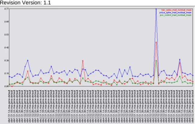
Figure 4: The mean absolute deviation of residuals reveals a consistent picture between the positive controls (green), bacterial spikes (red), and the polyA spikes (blue). All show the same chip from site 5 as a clear outlier. The same target from that chip was run on other chips in this data set, which suggests that the problem is probably with the chip itself versus a hybridization or sample problem.

One of the major root causes of outlier chips is the the quality and nature of the starting RNA material. In this case, this is very unlikely given that the same RNA is used in the whole study. Other causes include errors or problems with the target preparation (again unlikely in this case, as the same target is being hybridized to multiple chips), problems with hybridization and wash phase, or problems with scanning and gridding. The bacterial spikes, polyA spikes, and positive controls can be used to identify which of these problems is the likely reason for the outlier array.

In this case the replicate nature of the experimental design rules out the RNA sample and the target preparation. By deduction, the hybridization and fluidics methods as well as the chip itself are left as the only probable sources of the problems seen with this chip. The lack of problems observed on other chips from the same site suggests that the hybridization and wash steps are probably not the problem.

In the absence of replication information, the bacterial and polyA spikes can be used to assess this. If the bacterial spikes display the expected rank order (BioB<BioC<BioD<Cre) , then the problem is likely to be before the hybridization phase. If the polyA spikes display the expected rank order (lys<phe<thr<dap) then the problem is likely to be with the RNA sample or the target prep.

(11)

Figure 5: The rank order of the polyA spikes is as expected. Note the compromised signal value separation on the poor performing chip from site 5. Because the same complex background is used for all of these samples (same batch of HeLa RNA), the polyA spikes show more

consistency than is observed across very different sample types (Figure 10).

Within EC, the signal values for individual probesets can be visualized. In Figure 5 the signal values for the polyA spikes are shown. The expected rank orders of the spikes are observed and the problem with the outlier from site 5 is clearly seen at the individual probeset level.

(12)

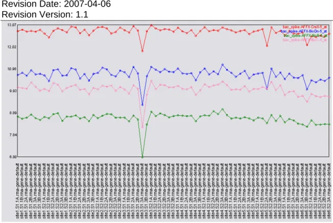
Figure 6: The rank order of the bacterial spikes is as expected. Note the slightly compromised signal value separation on the poor performing chip from site 5. More noticeable is a problem with the bacterial spikes on one of the chips from site 3, however the corresponding metrics for the polyA spikes and positive controls look fine, suggesting that the problem with the bacterial spikes is specific to just these controls (ie pipetting error) and not the whole chip. Because the same complex background is used for all of these samples (same batch of HeLa RNA), the bacterial spikes show more consistency than is observed across very different sample types (Figure 11).

In Figure 6 the bacterial spikes show a similar pattern to that of the polyA spikes in Figure 5. The expected rank order of the spikes are observed, however the problem with the outlier chip from site 5 is less apparent. There does appear to be a problem with the bacterial spikes on one of the chips from site 3. This problem appears to be isolated just to the spikes and may indicate a pipetting error.

The examination of the bacterial spikes, the polyA spikes, and the positive controls all show problems with this chip (Figure 4) suggesting that the quality of this specific chip is questionable. In conclusion, the replicate nature of this experiment and the utilization of different quality assessment metrics suggest that the problem is either in the hybridization, wash, or with the chip itself. If this was an important sample for which one needed the data, a rehybridization on a new chip with the existing target would be appropriate.

Multiple Target Prep Reactions

This example consists of multiple target preparation reactions done on different samples in the same lab. The Human Exon 1.0 ST Array was used for this example. An exon level analysis with PLIER was run on these chips.

(13)

Revision Version: 1.1 0 0.05 0.1 0.15 0.2 0.25 0.3 0.35 0.4

1 2 3 4 5 6 7 8 9 ₁₀ ₁₁ ₁₂ ₁₃ ₁₄ ₁₅ ₁₆ ₁₇ ₁₈ ₁₉ ₂₀ ₂₁ ₂₂ ₂₃ ₂₄

Ba

c

Po

lyA _Pos

Array

Mean Absolute Deviation Residuals

bac_spike_mad_residual_mean polya_spike_mad_residual_mean pos_control_mad_residual_mean

Figure 7: Target Prep Problem. This figure shows mean absolute deviation of residuals from PLIER model fit. This is for a data set with different samples run over the Human Exon 1.0 ST array. The samples are sorted based on the pos_control_mad_residual_mean. The median values plus/minus 2 standard deviations is shown to the right. The bacterial spikes are within the expected values while the polyA and positive controls reveal clear outliers; this suggests a problem with the target prep phase. Note that severe input RNA quality problems can affect the polyA and bacterial spikes due to the normalization step.

In this particular date set, the mean absolute deviation of residuals for the positive controls appeared unusually high for 6 of the chips (Figure 7). The problem can be isolated to the target prep phase by examining this metric for the bacterial spikes, the polyA spikes, and the positive controls. In this case the bacterial spikes, while variable, appear to fall within the expected range for all the chips. In contrast, the polyA spikes show higher residuals for the 6 chips in

question, consistent with the higher residuals observed for the positive controls. Thus the problem is likely with the target prep for those chips or the

quality/nature of the samples put on those chips. It is worth noting that

particularly bad starting RNA could affect the polyA and bacterial spikes because of distortions such a sample might introduce when normalizing the probe

intensities.

V.B. Tissue Panel Data Set

In this particular data set we have 3 biological replicates for 11 tissues. In addition, we’ve added 3 technical replicates for a HeLa sample from two sites including the outlier chip shown in Figure 1. This will demonstrate how a poor quality chip might appear in a more diverse data set.

(14)

Figure 8: In spite of the additional variability of dealing with tissue samples (as opposed to just cell lines) and biological variability within the replicates (as opposed to just technical variability) the same problematic chip can be clearly distinguished (HeLa Set 2 number 02) as an outlier.

In this case, where a large amount of variation is expected between samples the mean absolute deviation of the residuals is a good starting point. In Figure 8 the mean absolute deviation of residuals for all the probesets, the positive controls, the polyA spikes, and the bacterial spikes are shown. The outlier chip from site 5 (now labeled HeLa Set 2 Number 02) is still a clear outlier, particularly when compared to the other HeLa samples. The difference observed is smaller in magnitude when compared to the other tissues, but still apparent.

(15)

Figure 9: When dealing with more substantial biological variability (as is seen when looking across different tissues) the relative log expression metric becomes less useful. Many probesets are changing between the different tissues and as a result the mean absolute relative log expression is both high and variable across this data set.

As anticipated, do to the expected differences in signal between the different tissues, the mean absolute relative log expression is less useful for assessing quality in this diverse data set. This can be clearly seen by comparing the

graphs of the RLE for the positive controls in this data set (Figure 9) with a graph of the RLE for all probes in the data set focused on HeLa replicates (Figure 1). If one focuses on the mean absolute RLE for all the probesets (Figure 9, red line) you can see a general trend where a typical value is associated with each of the tissue trios. This would probably become clearer if more replicates were present for each tissue.

(16)

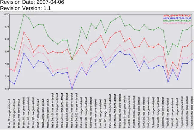
Figure 10: Unlike a data set consisting of primarily technical and biological replicates, the tissue panel shows a greater variability in the signal values reported for the polyA spikes. This is probably due (at least in part) to a breakdown in the assumption of identical intensity distributions between the different tissues. As a result the quantile normalization may be distorting the signal values.

When looking at the individual probeset values for the polyA spikes (Figure 10) and the bacterial spikes (Figure 11) a consistent rank order is observed for the spikes. The signal values reported for the spikes are more variable (than in Figure 5 and Figure 6) probably due to the diverse nature of the tissues included in this data set. In particular, the quantile normalization assumes identical

intensity profiles between the different tissues and this is probably not a valid assumption.

(17)

Figure 11 Unlike a data set consisting of primarily technical and biological replicates, the tissue panel shows a greater variability in the signal values reported for the bacterial spikes. This is probably due (at least in part) to a breakdown in the assumption of identical intensity distributions between the different tissues. As a result the quantile normalization may be distorting the signal values.

Conclusions

This paper demonstrates how some simple measures can be derived from array data to assess quality. The mean absolute relative log expression, mean

absolute deviation of residuals, and the positive vs negative ROC AUC are useful metrics to assess the overall data quality. When drilling into the various probeset categories, these metrics can be useful to isolate data quality problems to

specific stages of the microarray experiment.

One of the most critical aspects of generating a good microarray data set is experimental design and in particular the inclusion of an appropriate number of biological replicates for the purpose of the experiment. Additional biological replicates will not only increase the power of your study, but it will also make the job of quality assessment easier. As seen here, picking out a poor sample from a larger set of replicates (Figure 1, blue line) is easier than situations with relatively few replicates (Figure 8, red line).

Many of the quality assessment measures will be highly correlated. For the purpose of identifying gross outliers that should be excluded from downstream analysis most of the metrics discussed above will do a good job. Better methods – methods that are sensitive to departures in quality that have impact on

(18)

particular downstream analyses – must by their very nature be developed on a case by case basis.

V.C. References

Robert Gentleman, Vince Carey, Wolfgang Huber, Rafael Irizarry, Sandrine Dudoit, Bioinformatics and Computational Biology Solutions using R and