Recent Developments and Future Trends in
Visual Quality Assessment
Tsung-Jung Liu*, Weisi Lin† and C.-C. Jay Kuo*
*Ming Hsieh Department of Electrical Engineering, University of Southern California, Los Angeles, CA 90089, USA
E-mail: [email protected], [email protected] Tel: +1-213-7404658
† School of Computer Engineering, Nanyang Technological University, Singapore 639798, Singapore
E-mail: [email protected] Tel: +65-67906651 Abstract— The visual quality assessment approaches and their
classification are introduced. Recent developments on both image and video quality metrics, as well as several publicly available databases for both images and videos, are reviewed. Then, we conduct experiments on image and video quality databases to compare the performance of some existing state-of-the-art visual quality metrics. It is shown that multi-metric fusion (MMF) and motion-based video integrity evaluation (MOVIE) are the best methods for image and video quality assessment, respectively. Finally, future trends in visual quality assessment are discussed.
I. INTRODUCTION
In recent years, digital images and videos play more and more important roles in our work and life because of the availability and accessibility to the general public. Thanks to the rapid advancement of new technology, people can easily have an image/video capturing device, such as a digital camera and camcorder, to capture what they see and what happen in daily life. In addition, with the development of social network and mobile devices, photo and video sharing on the Internet becomes much popular and simpler than before. Hence, the quality assessment and assurance for digital images and videos in an objective manner become an increasingly useful and interesting topic in the research community.
Generally speaking, visual quality assessment can be divided into two categories. One is subjective visual quality assessment, and the other is objective visual quality assessment. As the name suggests, subjective quality assessment is done by humans. It represents the most realistic opinion of humans towards an image or a video, and also the most reliable measure of visual quality among all available means (if the pool of subjects is sufficiently large and the nature of the circumstances allows such assessment).
For subjective evaluation of visual quality, the tests can be performed with the methods defined in [1], [2]: (a) Pair Comparison (PC); (b) Absolute Category Rating (ACR); (c) Degradation Category Rating (DCR) (also called Double-Stimulus Impairment Scale (DSIS)); (d) Double-Double-Stimulus Continuous Quality Scale (DSCQS); (e) Single-Stimulus Continuous Quality Evaluation (SSCQE); (f) Simultaneous Double-Stimulus for Continuous Evaluation (SDSCE). We have presented these methods in Appendix for easy reference.
In general, Methods (a) ~ (c) can be used in multimedia applications. Television pictures can be evaluated with Methods (c) ~ (f). In all these test methods, the visual quality ratings evaluated by the test subjects are then averaged to
obtain the Mean Opinion Score (MOS). In some cases, Difference Mean Opinion Score (DMOS) is used to represent the mean of differential subjective score instead of MOS.
However, the subjective method is tedious, time-consuming, and not applicable for real-time processing since the test has to be performed with great care in order to obtain meaningful results. Moreover, it is not feasible to have human intervention with in-loop and on-service processes (like video encoding, transmission, etc.). Hence, more and more research has been focused on automatic assessment of quality for an image or a video. An objective visual quality metric can be standalone or embedded into algorithms, processes and systems that require it to boost the performance in terms of user (human) relevancy.
This paper aims at an overview and discussion of the latest existing research in the area of objective quality evaluation of visual signal (both image and video), and is organized as follows. In Section II, the classification of objective quality assessment methods will be presented. Recent developments and publicly available databases in image quality assessment (IQA) will be introduced in Section III, while those in video quality assessment (VQA) are to be introduced in Section IV. Section V will present performance comparison for the recent popular visual quality metrics. Then we will address several possible future trends for visual quality assessment in Section VI. Finally, the conclusion will be drawn in Section VII.
II. CLASSIFICATION OF OBJECTIVE VISUAL QUALITY
ASSESSMENT METHODS
There are several popular ways to classify the visual quality assessment methods [3], [4], [5]. In this section, we present two possibilities of classification to facilitate the presentation and understanding of the related problems, the existing solutions and the future trends in development.
A. Classification Based upon the Availability of Reference
The classification depends on the availability of original (reference) image/video. If there is no reference signal available for the distorted (test) one to compare with, then a quality evaluation method is termed as a no-reference (NR) one [6]. The current NR method does not perform well in general since it judges the quality solely based on the distorted medium and without any reference available. However, it can be used in wider scope of applications because of its suitability in both situations with and without reference information; the computational requirement is APSIPA ASC 2011 Xi’an
usually less since there is no need to process the reference. Besides the traditional NR cases (like the relay site and receiving end of transmission), there are emerging NR applications (e.g., super-resolution construction, image and video retargeting/adaption, and computer graphics/animation).
If the information of the reference medium is partially available, e.g., in the form of a set of extracted features, then this is the so-called reduced-reference (RR) method [7]. Since the extracted partial reference information is much sparser than the whole reference, the RR approach can be used in a remote location (e.g., the relay site and receiving end of transmission) with reasonable bandwidth overheads to achieve better results than the NR method, or in a situation where the reference is available (such as a video encoder) to reduce computational requirement (especially in repeated manipulation and optimization).
The last one is the full-reference (FR) method (e.g., [8]), as the opposite of the NR method. As the name suggests, an FR metric needs the complete reference medium to assess the distorted medium. Since it has the full information about original medium, it is expected to have the best quality prediction performance. Most existing quality assessment schemes belong to this category. We will discuss more in Sections III and IV.
B. Classification Based upon Methodology for Assessment
The first type in this classification is image/video fidelity metrics, which operate based only on the direct accumulation of physical errors and are therefore usually FR ones. Mean-squared error (MSE) and peak signal-to-noise ratio (PSNR) are two representatives in this category. Although being the simplest and still widely used, such a metric is often not a good reflection of perceived visual quality if the distortion is not additive.
The second type is the human visual system (HVS) model based metrics, which typically employ a frequency-based decomposition, and take into account various aspects of the HVS. This can include modeling of contrast and orientation sensitivity, spatial and temporal masking effects, frequency selectivity and color perception. Due to the complexity of the HVS, these metrics can become very complex and computationally expensive. Examples of the work following this framework include the work in [9], Perceptual Distortion Metric (PDM) [10], the continuous video quality metric in [11] and the scalable wavelet based video distortion index [12].
Signal structure, information or feature extracted metrics are the third type of metrics. Some of them quantify visual fidelity based on the assumption that a high-quality image or video is one whose structural content, such as object boundaries or regions of high entropy, most closely matches that of the original image or video [8], [13], [14]. Other metrics of this type are based on the idea that the HVS understands an image mainly through its low-level features. Hence, image degradations can be perceived by comparing the low-level features between the distorted and the reference images. The latest work is called feature-similarity (FSIM)
index [15]. We will discuss more details on this type of metric in Section III.
The last type of metrics is the emerging learning-oriented metrics. Some recent works are [16], [17], [18], [19], [20]. Basically, it extracts the specific features from the image or video, and then uses the machine learning approach to obtain a trained model. Finally, they use this trained model to predict the perceived quality of images/videos. The obtained experimental results are quite promising, especially for multi-metric fusion (MMF) approach [19] which uses the major existing metrics (including SSIM, MS-SSIM, VSNR, IFC, VIF, PSNR, and PSNR-HVS) as the components for the learnt model. The MMF is expected to outperform all the existing metrics because it is the fusion-based approach and allows the combination of merits of each metric.
III. RECENT DEVELOPMENTS IN IQA
A. Image quality databases
Databases with subjective data facilitate metric development and benchmarking. There are a number of publicly available image quality database, including LIVE [21], TID2008 [22], CSIQ [23], IVC [24], IVC-LAR [25], Toyoma [26], WIQ [27], A57 [28], and MMSP 3D Image [29]. We will give a brief introduction for each database below.
LIVE Image Quality Database has 29 reference images (also called source reference circuits (SRC)), and 779 test images, including five distortion types - JPEG2000, JPEG, white noise in the RGB components, Gaussian blur, and transmission errors in the JPEG2000 bit stream using a fast-fading Rayleigh channel model. The subjective quality scores provided in this database are DMOS, ranging from 0 to 100.
Tampere Image Database 2008 (TID2008) has 25 reference images, and 1700 distorted images, including 17 types of distortions and 4 different levels for each type of distortion. Hence, there are 68 test conditions (also called hypothetical reference circuits (HRC)). MOS is provided in this database, and the scores range from 0 to 9.
Categorical Image Quality (CSIQ) Database contains 30 reference images, and each image is distorted using 6 types of distortions - JPEG compression, JPEG2000 compression, global contrast decrements, additive Gaussian white noise, additive Gaussian pink noise, and Gaussian blurring - at 4 to 5 different levels, resulting in 866 distorted images. The score ratings (0 to 1) are reported in the form of DMOS.
IVC Database has 10 original images, and 235 distorted images, including 4 types of distortions – JPEG, JPEG2000, locally adaptive resolution (LAR) coding, and blurring. The subjective quality scores provided in this database are MOS, ranging from 1 to 5.
IVC-LAR Database contains 8 original images (4 natural images, and 4 art images), and 120 distorted images, including three distortion types – JPEG, JPEG2000, and LAR coding. The subjective quality scores provided in this database are MOS, ranging from 1 to 5.
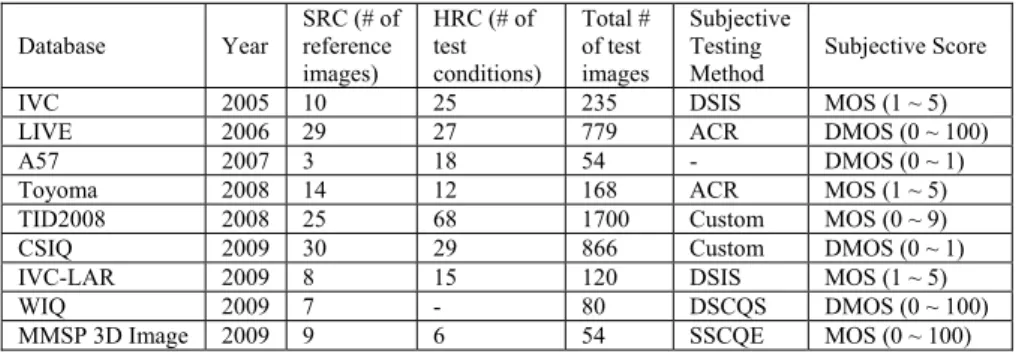
TABLE 1: COMPARISON OF IMAGE QUALITY DATABASES
(notes: ‘-‘ means no information available; ‘Custom’ means the testing method is designed by the authors, not in [1] and [2].) Database Year SRC (# of reference images) HRC (# of test conditions) Total # of test images Subjective Testing Method Subjective Score
IVC 2005 10 25 235 DSIS MOS (1 ~ 5)
LIVE 2006 29 27 779 ACR DMOS (0 ~ 100)
A57 2007 3 18 54 - DMOS (0 ~ 1)
Toyoma 2008 14 12 168 ACR MOS (1 ~ 5)
TID2008 2008 25 68 1700 Custom MOS (0 ~ 9)
CSIQ 2009 30 29 866 Custom DMOS (0 ~ 1)
IVC-LAR 2009 8 15 120 DSIS MOS (1 ~ 5)
WIQ 2009 7 - 80 DSCQS DMOS (0 ~ 100)
MMSP 3D Image 2009 9 6 54 SSCQE MOS (0 ~ 100)
Toyoma Database has 14 original images, and 168 distorted images, including two types of distortions – JPEG, and JPEG2000. The subjective scores in this database are MOS, ranging from 1 to 5.
Wireless Imaging Quality (WIQ) Database has 7 reference images, and 80 distorted images. The subjective quality scores used in this database are DMOS, ranging from 0 to 100.
A57 Database has 3 original images, and 54 distorted images, including six distortion types - quantization of the LH subbands of a 5-level DWT of the image using the 9/7 filters, additive Gaussian white noise, JPEG compression, JPEG2000 compression, JPEG2000 compression with the Dynamic Contrast-Based Quantization (DCQ), and Gaussian blurring. The subjective quality scores used for this database are DOMS, ranging from 0 to 1.
MMSP 3D Image Quality Assessment Database contains stereoscopic images with a resolution of 1920x1080 pixels. Various indoor and outdoor scenes with a large variety of colors, textures, and depth structures have been captured. The database contains 10 scenes. Seventeen subjects participated in the test. For each of the scenes, 6 different stimuli have been considered corresponding to different camera distances (10, 20, 30, 40, 50, 60 cm).
To make a clear comparison among these databases, we list the important information for each database in Table 1.
B. Major IQA metrics
As mentioned earlier, the simplest and most widely used image quality metrics are MSE and PSNR since they are easy to calculate and are also mathematically convenient in the context of optimization. However, they often correlate poorly with subjective visual quality [30].
Hence, researchers have done a lot of work to include the characteristics of the HVS to improve the performance of the quality prediction. The noise quality measure (NQM) [31], PSNR-HVS-M [32], and the visual signal-to-noise ratio (VSNR) [33] are several representatives in this category.
NQM (FR, HVS model based metric), which is based on Peli’s contrast pyramid [34], takes into account the following:
1) variation in contrast sensitivity with distance, image dimensions, and spatial frequency;
2) variation in the local luminance mean;
3) contrast interaction between spatial frequencies;
4) contrast masking effects.
It has been demonstrated that the nonlinear NQM is a better measure of additive noise than PSNR and other linear quality measures [31].
PSNR-HVS-M (FR, HVS model based metric) is a still image quality metric which takes into account contrast sensitivity function (CSF) and between-coefficient contrast masking of DCT basis functions. It has been shown that PSNR-HVS-M outperforms other well-known reference based quality metrics and demonstrated high correlation with the results of subjective experiments [32].
VSNR (FR, HVS model based metric) is a metric computed by a two-stage approach [33]. In the first stage, contrast thresholds for detection of distortions in the presence of natural images are computed via wavelet-based models of visual masking and visual summation in order to determine whether the distortions in the distorted image are visible. If the distortions are below the threshold of detection, the distorted image is claimed to be of perfect visual quality. If the distortions are higher than a threshold, a second stage is applied, which operates based on the visual property of perceived contrast and global precedence. These two properties are modeled as Euclidean distances in distortion-contrast space of a multi-scale wavelet decomposition, and final VSNR is obtained based on a simple linear summation of these distances.
However, the HVS is a complex and highly nonlinear system, and most models so far are only based on linear or quasi-linear operators. Hence, a different framework was introduced, based on the assumption that a measurement of structural information change should provide a good approximation to perceived image distortion. Structural similarity (SSIM) index (FR, Signal structure extracted metric) [8] is the most well-known one in this category.
Suppose two image signals x and y, and let , , 2, 2
y x y x
andxybe the mean of x, the mean of y, the variance of x, the variance of y, and the covariance of x and y respectively. Wang et al. [8] define the luminance, contrast and structure comparison measures as follows:
1 2 2 1 2 ) ( C C l y x y x y x, , 2 2 2 2 2 ) ( C C c y x y x y x, ,
3 3 ) ( C C s y x xy y x, ,
where the constants C1, C2,, C3 are included to avoid
instabilities when x2y2, x2y2, and xy are very close to zeroes. Finally, they combine these three comparison measures and name the resulting similarity measure between image signals x and y as
[ ( , )] [ ( , )] )] , ( [ ) , ( SSIM x y l x y cx y s x y
where 0, 0 and 0 are the parameters used to adjust the relative importance of these three components. In order to simplify the expression, they set 1 and
2 /
2
3 C
C . This results in a specific form of the SSIM index between image signals x and y:
) )( ( ) 2 )( 2 ( ) ( SSIM 2 2 2 1 2 2 2 1 C C C C y x y x xy y x y x,
However, SSIM is only a single-scale method. To be able to incorporate image details at different resolutions, a multi-scale SSIM (MS-SSIM) (FR, Signal structure extracted metric) [35] is adopted. Taking the reference and distorted image signals as the input, the system iteratively applies a low-pass filter and down-samples the filtered image by a factor of two. They index the original image as scale 1, and the highest scale as scale M, which is obtained after M - 1 iterations. At the j-th scale, the contrast comparison and the structure comparison are calculated and denoted as cj (x,y) and sj (x,y), respectively. The luminance comparison is computed only at scale M and denoted as lM (x,y). The overall SSIM evaluation is obtained by combining the measurement at different scales using
MS-
M j j j M j j M c s l 1 )] , ( [ )] , ( [ )] , ( [ ) , ( SSIM x y x y x y x y Similarly, the exponents M, j and j are used to adjust
the relative importance of different components. To simplify parameter selection, they let j j j for all j’s. In
addition, they also normalize the cross-scale settings such that
M
j1j 1.
Since SSIM is sensitive to relative translations, rotations, and scalings of images [30], complex-wavelet SSIM (CW-SSIM) [36] is developed. The CW-SSIM is locally computed from each subband, and then averaged over space and subbands, yielding an overall CW-SSIM index between the original and the distorted images. The CW-SSIM method is robust with respect to luminance changes, contrast changes and translations [36].
Afterward, some researchers have tried to propose a new metric by modifying SSIM, such as 3-component weighted SSIM (3-SSIM) [37], and information content weighted SSIM (IW-SSIM) [38]. They are all based on the similar strategy to assign different weightings to the SSIM scores.
Another metric based on the information theory to measure image fidelity is called information fidelity criterion (IFC) (FR, Signal information extracted metric) [13]. It was later extended to visual information fidelity (VIF) metric (FR, Signal information extracted metric) [14]. The VIF attempts to relate signal fidelity to the amount of information that is shared between two signals. The shared information is quantified using the concept of mutual information. The reference image is modeled by a wavelet domain Gaussian scale mixture (GSM), which has been shown to model the non-Gaussian marginal distributions of the wavelet coefficients of natural images effectively, and also capture the dependencies between the magnitudes of neighboring wavelet coefficients. Therefore, it brings good performance to the VIF index over a wide range of distortion types [39].
FSIM (FR, Signal feature extracted metric) [15] is a recently developed image quality metric, which compares the low-level feature sets between the reference image and the distorted image based on the fact that the HVS understands an image mainly according to its low-level features. Phase congruency (PC) is the primary feature to be used in computing FSIM. Gradient magnitude (GM) is the second feature to be added in FSIM metric because PC is contrast invariant and contrast information also affects the HVS’ perception of image quality. Actually, in the FSIM index, the similarity measures for PC and GM all follow the same formula as in the SSIM metric.
IV. RECENT DEVELOPMENTS IN VQA
A. Video quality databases
To our knowledge, there are nine public video quality databases available, including VQEG FRTV-I [40], IRCCyN/IVC 1080i [41], IRCCyN/IVC SD RoI [42], EPFL-PoliMI [43], LIVE [44], LIVE Wireless [45], MMSP 3D Video [46], MMSP SVD [47], VQEG HDTV [48]. We will briefly introduce them below.
VQEG FR-TV Phase I Database is the oldest public database on video quality applied to MPEG-2 and H.263 video with two formats: 525@60Hz and 625@50Hz in this database. The resolution for video sequence 525@60Hz is 720x486 pixels, and 720x576 pixels for 625@50Hz. The video format is 4:2:2. And the subjective quality scores provided are DMOS, ranging from 0 to 100.
IRCCyN/IVC 1080i Database contains 24 contents. For each content, there is one reference and seven different compression rates on H.264 video. The resolution is 1920x1080 pixels, the display mode is interleaving and the field display frequency is 50Hz. The provided subjective quality scores are MOS, ranging from 1 to 5.
IRCCyN/IVC SD RoI Database contains 6 reference videos and 14 HRCs (i.e., 84 videos in total). The HRCs are H.264 coding with or without error transmission simulations. The contents of this database are SD videos. The resolution is 720x576 pixels, the display mode is interleaving and the field display frequency is 50Hz with MOS from 1 to 5.
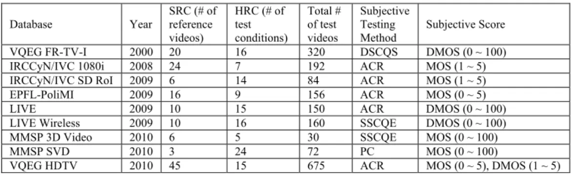
TABLE 2: COMPARISON OF VIDEO QUALITY DATABASES Database Year SRC (# of reference videos) HRC (# of test conditions) Total # of test videos Subjective Testing Method Subjective Score
VQEG FR-TV-I 2000 20 16 320 DSCQS DMOS (0 ~ 100)
IRCCyN/IVC 1080i 2008 24 7 192 ACR MOS (1 ~ 5)
IRCCyN/IVC SD RoI 2009 6 14 84 ACR MOS (1 ~ 5)
EPFL-PoliMI 2009 16 9 156 ACR MOS (0 ~ 5)
LIVE 2009 10 15 150 ACR DMOS (0 ~ 100)
LIVE Wireless 2009 10 16 160 SSCQE DMOS (0 ~ 100)
MMSP 3D Video 2010 6 5 30 SSCQE MOS (0 ~ 100)
MMSP SVD 2010 3 24 72 PC MOS (0 ~ 100)
VQEG HDTV 2010 45 15 675 ACR MOS (0 ~ 5), DMOS (1 ~ 5)
EPFL-PoliMI Video Quality Assessment Database contains 12 reference videos (6 in CIF, and 6 in 4CIF), and 144 distorted videos, which are encoded with H.264/AVC and corrupted by simulating the packet loss due to transmission over an error-prone network. For CIF, the resolution is 352x288 pixels, and frame rate 30fps. For 4CIF, the resolution is 704x576 pixels, and frame rate are 30fps and 25fps. For each of the 12 original H.264/AVC videos, they have generated a number of corrupted ones by dropping packets according to a given error pattern. To simulate burst errors, the patterns have been generated at six different packet loss rates (PLR) and two channel realizations have been selected for each PLR.
LIVE Video Quality Database includes 10 reference videos. All videos are 10 seconds long, except for Blue Sky. The Blue Sky sequence is 8.68 seconds long. The first seven sequences have a frame rate of 25 fps, while the remaining three (Mobile & Calendar, Park Run, and Shields) have a frame rate 50 fps. There are 15 test sequences from each of the reference sequences using four different distortion processes – simulated transmission of H.264 compressed videos through error-prone wireless networks and through error-prone IP networks, H.264 compression, and MPEG-2 compression. All video files have planar YUV 4:2:0 formats and do not contain any headers. The spatial resolution of all videos is 768x432 pixels.
LIVE Wireless Video Quality Assessment Database has 10 reference videos, and 160 distorted videos, which focus on H.264/AVC compressed video transmission over wireless networks. The video is YUV 4:2:0 formats with a resolution of 768x480 and a frame rate of 30 fps. Four bit-rates and 4 packet-loss rates are performed. However, this database has been taken offline temporarily since it has limited video contents and a tendency to cluster at 0.95~0.96 correlation level for most objective metrics.
MMSP 3D Video Quality Assessment Database contains stereoscopic videos with a resolution of 1920x1080 pixels and a frame rate of 25 fps. Various indoor and outdoor scenes with a large variety of color, texture, motion, and depth structure have been captured. The database contains 6 scenes, and 20 subjects participated in the test. For each of the scenes, 5 different stimuli have been considered corresponding to different camera distances (10, 20, 30, 40, 50 cm).
MMSP Scalable Video Database is related to 2 scalable video codecs (SVC and wavelet-based codec), 3 HD contents,
and bit-rates ranging between 300 kbps and 4 Mbps. There are 3 spatial resolutions (320x180, 640x360, and 1280x720), and 4 temporal resolutions (6.25 fps, 12.5 fps, 25 fps and 50 fps). In total, 28 and 44 video sequences were considered for each codec, respectively. The video data are in the YUV 4:2:0 formats.
VQEG HDTV Database has 4 different video formats – 1080p at 25 and 29.97fps, 1080i at 50 and 59.94fps. The impairments are restricted to MPEG-2 and H.264, with both coding-only error and coding-plus-transmission error. The video sequences are released progressively via the Consumer Digital Video Library (CDVL) [49].
We summarize and compare these video quality databases in Table 2 for the convenience of the readers.
B. Major VQA metrics
One obvious way to implement video quality metrics is to apply a still image quality assessment metric on a frame-by-frame basis. The quality of each frame-by-frame is evaluated independently, and the global quality of the video sequence can be obtained by a simple time average.
SSIM has been applied in video quality assessment as reported in [50]. The quality of the distorted video is measured in three levels: the local region level, the frame level, and the sequence level. First, the SSIM indexing approach is applied to the Y, Cb and Cr color components independently and combined into a local quality measure using a weighted summation. In the second level of quality evaluation, the local quality values are weighted to obtain a frame level quality index. Finally in the third level, the overall quality of the video sequence is given by the weighted summation of the frame level quality index. This approach is often called as V-SSIM (FR, Signal structure extracted metric), and has been demonstrated to perform better than KPN/Swisscom CT [51] (the best metric for the Video Quality Experts Group (VQEG) Phase I test data set [40]) in [50].
Wang and Li [52] proposed Speed-SSIM (FR, Signal structure extracted metric) that incorporated a model of the human visual speed perception by formulating the visual perception process in an information communication framework. Consistent improvement over existing VQA algorithms has been observed in the validation with the VQEG Phase I test data set [40].
Watson et al. [53] developed a video quality metric, which they call digital video quality (DVQ) (FR, HVS model based metric). The DVQ accepts a pair of video sequences, and computes a measure of the magnitude of the visible difference between them. The first step consists of various sampling, cropping, and color transformations that serve to restrict processing to a region of interest and to express the sequence in a perceptual color space. This stage also deals with de-interlacing and de-gamma-correcting the input video. The sequence is then subjected to a blocking and a DCT, and the results are transformed to local contrast. The next steps are temporal and spatial filtering, and a contrast masking operation. Finally, the masked differences are pooled over spatial temporal and chromatic dimensions to compute a quality measure.
Video Quality Metric (VQM) (RR, HVS model based metric) [7] is developed by National Telecommunications and Information Administration (NTIA) to provide an objective measurement for perceived video quality. The NTIA VQM provides several quality models, such as the Television Model, the General Model, and the Video Conferencing Model, based on the video sequence under consideration and with several calibration options prior to feature extraction in order to produce efficient quality ratings. The General Model contains seven independent parameters. Four parameters (si_loss, hv_loss, hv_gain, si_gain) are based on the features extracted from spatial gradients of Y luminance component, two parameters (chroma_spread, chroma_extreme) are based on the features extracted from the vector formed by the two (Cb, Cr) chrominance components, and one parameter (ct_ati_gain) is based on the product of features that measure contrast and motion, both of which are extracted from Y luminance component. The VQM takes the original video and the processed video as inputs and is computed using the linear combination of these seven parameters. Due to its performance in the VQEG Phase II validation tests, the VQM method was adopted as a national standard by the American National Standards Institute (ANSI) and as International Telecommunications Union Recommendations [54], [55].
By analyzing subjective scores of various video sequences, Lee et al. [56] found out that the HVS is sensitive to degradation around edges. In other words, when edge areas of a video sequence are degraded, evaluators tend to give low quality scores to the video, even though the overall mean squared error is not large. Based on this observation, they propose an objective video quality measurement method based on degradation around edges. In the proposed method, they first apply an edge detection algorithm to videos and locate edge areas. Then, they measure degradation of those edge areas by computing mean squared errors and use it as a video quality metric after some post-processing. Experiments show that this proposed method EPSNR (FR, Video fidelity metric) outperforms the conventional PSNR. This method was also evaluated by independent laboratory groups in the VQEG Phase II test. As a result, it was included in international recommendations for objective video quality measurement [56].
More recently, an approach integrates both spatial and temporal aspects of distortion assessment, known as MOtion-based Video Integrity Evaluation (MOVIE) index (FR, HVS model based metric) [57]. The MOVIE uses optical flow estimation to adaptively guide spatial-temporal filtering using three-dimensional (3-D) Gabor filterbanks. The key difference of this method is that a subset of filters are selected adaptively at each location based on the direction and speed of motion, such that the major axis of the filter set is oriented along the direction of motion in the frequency domain. The video quality evaluation process is carried out with coefficients computed from these selected filters only. One component of the MOVIE framework, known as the Spatial MOVIE index, uses the output of the multi-scale decomposition of the reference and test videos to measure spatial distortions in the video. The second component of the MOVIE index, known as the Temporal MOVIE index, captures temporal degradations in the video. The Temporal MOVIE index computes and uses motion information from the reference video explicitly in quality measurement, and evaluates the quality of the test video along the motion trajectories of the reference video. Finally, the Spatial MOVIE index and the Temporal MOVIE index are combined to obtain a single measure of video quality known as the MOVIE index. The performance of MOVIE on the VQEG FRTV Phase I dataset is summarized in [57].
In addition, TetraVQM (FR, HVS model based metric) [58] has been proposed to utilize motion estimation within a VQA framework, where motion compensated errors are computed between the reference and distorted images. Based on the motion vectors and the motion prediction error, the appearance of new image areas and the display time of objects are evaluated. Additionally, degradations which happen to moving objects can be judged more exactly. And in [59], Ninassi et al. tried to utilize models of visual attention and human eye movements to improve the VQA performance. The temporal variations of the spatial distortions are evaluated both at eye fixation level and on the whole video sequence. These two kinds of temporal variations are assimilated into a short-term temporal pooling and a long-term temporal pooling, respectively.
V. PERFORMANCE COMPARISON
We use the following three indexes to measure metric performance [51], [60]. The first index is the Pearson linear correlation coefficient (PLCC) between objective/subjective scores after non-linear regression analysis. It provides an evaluation of prediction accuracy. The second index is the Spearman rank order correlation coefficient (SROCC) between the objective/subjective scores. It is considered as a measure of prediction monotonicity. The third index is the root-mean-squared error (RMSE). Before computing the first and second indices, we need to use the logistic function and the procedure outlined in [51] to fit the objective model scores to the MOS (or DMOS). The monotonic logistic function used to fit the objective prediction scores to the subjective quality scores [51] is:
2 ) | 4 | 3 ( 2 1 1 ) ( x e x f
where x is the objective prediction score, f(x) is the fitted objective score, and the parameters j (j = 1,2,3,4) are chosen to minimize the least squares error between the subjective score and the fitted objective score. For an ideal match between the objective prediction scores and the subjective quality scores, PLCC=1, SROCC=1 and RMSE=0.
A. Image quality metric benchmarking
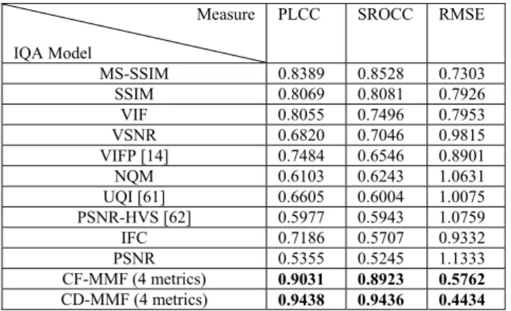
To examine the performance of existing popular image quality metrics in this work, we choose TID2008 to test image quality metrics since it includes the largest number of distorted images and also spans 17 distortion types, which covers most image distortion types that other publicly available image quality databases cannot provide. The performance results are listed in Table 3 with the three indices given above. The best performing metric is highlighted in bold. Clearly, MMF (both CF-MMF and CD-MMF) [19] have the highest PLCCs, SROCCs and the smallest RMSEs among the twelve image quality metrics under comparison. It demonstrates that the objective scores obtained by MMF have the highest correlation with human subjective scores. We will introduce more details about MMF in Section VI.
TABLE 3: COMPARISON OF THE PERFORMANCE OF IQA MODELS Measure IQA Model PLCC SROCC RMSE MS-SSIM 0.8389 0.8528 0.7303 SSIM 0.8069 0.8081 0.7926 VIF 0.8055 0.7496 0.7953 VSNR 0.6820 0.7046 0.9815 VIFP [14] 0.7484 0.6546 0.8901 NQM 0.6103 0.6243 1.0631 UQI [61] 0.6605 0.6004 1.0075 PSNR-HVS [62] 0.5977 0.5943 1.0759 IFC 0.7186 0.5707 0.9332 PSNR 0.5355 0.5245 1.1333 CF-MMF (4 metrics) 0.9031 0.8923 0.5762 CD-MMF (4 metrics) 0.9438 0.9436 0.4434
B. Video quality metric benchmarking
For the comparison of the state-of-the-art video quality metrics, LIVE Video Quality Database is adopted. Although most people use VQEG-FRTV Phase I Database (built in 2000) to test their metric performance previously, we decide to use LIVE Video Quality Database (released in 2009) as our test database since it is new and contains more distortion types, such as H.264 compression, simulated transmission of H.264 packetized streams through error prone wireless networks and error-prone IP networks, and MPEG-2 compression. The comparison results are summarized in Table 4. Here, the image quality metrics (i.e., PSNR, VSNR, SSIM, and MS-SSIM) are used on a frame-by-frame basis for the video sequence, and then time-averaging the frame scores to obtain the video quality score.
TABLE 4: COMPARISON OF THE PERFORMANCE OF VQA MODELS Measure VQA Model PLCC SROCC RMSE PSNR 0.5465 0.5205 9.1929 VSNR 0.6880 0.6714 7.9666 SSIM 0.5413 0.5233 9.2301 MS-SSIM 0.7551 0.7479 7.1963 V-SSIM 0.6058 0.5924 8.7337 VQM 0.7695 0.7529 7.0111 MOVIE 0.8116 0.7890 6.4130
From Table 4, we can conclude MOVIE is the best metric (which is highlighted in bold) for LIVE Video Quality Database, and VQM and MS-SSIM rank the second and third, respectively. It means that MOVIE correlates better with subjective results than other approaches under comparison. The MS-SSIM does not utilize any temporal information, and can still achieve reasonable good results. In general, the consideration of temporal structure and information, as well as the interaction of spatial and temporal features [63], can improve the video quality prediction performance.
VI. DISCUSSION ON FUTURE TRENDS
Although many visual quality assessment metrics have been developed for both image and video during the past decade, there are still great technological challenges ahead and much space for improvement, toward effective, reliable, efficient and widely accepted replacement for MSE/PSNR, for both standalone and embedded applications. We will discuss the possible directions in this section.
A. PSNR or SSIM-modified metrics
PSNR has always been criticized its poor correlation with human subjective evaluations. However, according to our observations [19], PSNR sometimes still can work very well on some specific distortion types, such as additive and quantization noise. Hence, a lot of metrics have been developed or derived from PSNR, such as PSNR-HVS-M [32], EPSNR [56], and SPHVSM [64]. They either incorporate some related HVS characteristics into PSNR or include some experimental observations to modify PSNR to improve the correlation. Promising results can be achieved in this way of modification. Among the quality metrics we just mentioned above, only the EPSNR is developed to use on video quality assessment.
As a single metric, the SSIM is considered the well-performed metric among all visual quality evaluation metrics, in terms of consistency. Thus, researchers in the field have managed to transform it by changing its pooling method or using other image features. Several examples of the former are V-SSIM [50], Speed-SSIM [52], 3-SSIM [37], and IW-SSIM [38], while FSIM index [15] is an example of the latter. They are all proven quite useful in improving the quality prediction performance, especially FSIM, which shows
superior performance in several image quality databases, including TID2008, CSIQ, LIVE, and IVC.
Building new metrics based upon more mature metrics (like PSNR and SSIM) is expected to continue, especially in new application scenarios (e.g., for 3D scenes, mobile media, medical imaging, image/video retargeting, computer graphics, and so on).
B. Multiple strategies or Multi-Metric Fusion approaches
In [65], Larson and Chandler suggested that a single strategy may not be sufficient to determine the image quality. They presented a quality assessment method, called most apparent distortion (MAD), which can model two different strategies. First, they used local luminance and contrast masking to estimate the detection-based perceived distortions in high quality images. Then changes in the local statistics of spatial-frequency components are used to estimate the appearance-based perceived distortions in low quality images. In the end, the authors showed that combining these two strategies can predict subjective ratings of image quality well.
More recently, we proposed a multi-metric fusion (MMF) approach for visual quality assessment [19]. This method is motivated by the observation that no single metric can give the best performance scores in all situations. To achieve MMF, a regression approach is adopted. First, we collected a large number of image samples, each of which has a score labeled by human observers and scores associated with different metrics. The new MMF score is set to be the nonlinear combination of scores obtained by multiple existing metrics (including SSIM, MS-SSIM, VSNR, IFC, VIF, PSNR, and PSNR-HVS) with suitable weights via a training process. We also call it as context-free MMF (CF-MMF) since it does not depend on image contexts. Furthermore, we divide image distortions into several groups and perform regression within each group, which is called context-dependent MMF (CD-MMF). One task in CD-MMF is to determine the context automatically, which is achieved by a machine learning approach. It is shown by experimental results that the proposed MMF metric outperforms all existing metrics by a significant margin.
Appropriate fusion of existing metrics opens the chances to build on the strength of each participating metric and the resultant framework can be even used when new, good metrics emerge. More careful and in-depth investigation is needed for this topic.
C. Migration from IQA to VQA
Up to now, more research has been performed for IQA. As mentioned before, video quality evaluation can be done by using image quality metrics on a frame-by-frame basis, and then averaging to obtain a final video quality score. However, this only works well when video contents do not have large motion in temporal domain. When there exist a large motion, we need to find out the temporal structure and temporal features.
The most common method is to use the motion estimation to find out the motion vectors and measure the variations in temporal domain. One simple realization of this idea is in
[66]. The authors extended one existing image quality assessment metric to a video quality metric by considering temporal information and converted it into a compensation factor to correct the video quality score obtained in the spatial domain. There are also other video quality metrics that utilize motion estimation to detect the temporal variations, such as Speed-SSIM [52], MOVIE [57], and TetraVQM [58]. All the above approaches improve the correlation between predictions and subjective quality scores more or less. This demonstrates that the temporal variation is indeed an important factor we need to consider for VQA.
Similarly, we can also use the MMF strategy on video quality assessment, via fusing the scores obtained from all available video quality metrics. A possible problem of this approach is the high complexity since multiple metrics and video data are involved. One solution to realize efficient MMF for video is to pick up the best features used in all metrics, including both spatial and temporal features, instead of using all participating metrics as they are. Moreover, this solution gives a chance to eliminate the repetition in feature detection among different metrics, and proper machine learning techniques will be customized for this purpose. In addition, visual attention modeling [67] may play a more active role in VQA than IQA.
D. Audiovisual Quality Assessment for 3G Networks
During the recent years, the term Quality of Experience (QoE) has been used and defined as the users’ perceived Quality of Service (QoS). More often than not in multimedia applications, the quality assessment has to be performed with audio and video (images) being presented together. It is an important but less investigated research topic, in spite of some early work in this area [68-70].
It has been proposed that a better QoE can be achieved when the QoS is considered both in the network and application layers as a whole [71]. In the application layer, QoS is affected by the factors such as resolution, frame rate, sampling rate, number of channels, color, video codec type, audio codec type, and layering strategy. The network layer introduces impairment parameters such as packet loss, jitter, network delay, burstiness, and decreased throughput, etc. These are all the key factors that affect the overall audiovisual QoE. Hence, to investigate into the quality assessment methods for both audio and video is also important and meaningful since video chats and video conferences over 3G networks may be frequently used by the general public in the near future.
Currently there is no public database for joint audiovisual quality and experience evaluation. The establishment of such databases will facilitate the research and promote the advancement in this field.
VII. CONCLUSION
In this paper, we have reviewed the existing visual quality assessment methods and their classification. Then we introduced the recent developments in image quality assessment (IQA), including the popular public image quality
databases that play an important role in boosting the research activities in this field and several well-performed image quality metrics. Similarly, we also discussed the recent developments for video quality assessment (VQA) in general, the publicly available video quality databases and several state-of-the-art VQA metrics. In addition, we have compared the major existing IQA and VQA metrics, and the experimental results showed that the MMF and the MOVIE outperform other metrics in the most comprehensive image and video quality databases respectively. In the end, we have presented several possible directions for future visual signal quality assessment, such as PSNR or SSIM-modified metrics, multiple strategy approaches, migration of IQA to VQA, and joint audiovisual assessment, with reasoning.
Appendix. Standard subjective testing methods [1], [2]. (a) Pair Comparison (PC)
The method of Pair Comparisons implies that the test sequences are presented in pairs, consisting of the same sequence being presented first through one system under test and then through another system.
(b) Absolute Category Rating (ACR)
The Absolute Category Rating method is a category judgment where the test sequences are presented one at a time and are rated independently on a discrete five-level scale from ‘bad’ to ‘excellent’. This method is also called Single Stimulus Method.
(c) Degradation Category Rating (DCR) (also called the Double-Stimulus Impairment Scale (DSIS))
The reference picture (sequence) and the test picture (sequence) are presented only once or twice. The reference is always shown before the test sequence, and neither is repeated. Subjects rate the amount of impairment in the test sequence on a discrete five-level scale from ‘very annoying’ to ‘imperceptible’.
(d) Double-Stimulus Continuous Quality Scale (DSCQS) The reference and test sequences are presented twice in alternating fashion, in the order of the two chosen randomly for each trial. Subjects are not informed which one is the reference and which one is the test sequence. They rate each of the two separately on a continuous quality scale ranging from ‘bad’ to ‘excellent’. Analysis is based on the difference in rating for each pair, which is calculated from an equivalent numerical scale from 0 to 100.
(e) Single-Stimulus Continuous Quality Evaluation (SSCQE) Instead of seeing separate short sequence pairs, subjects watch a program of 20~30 minutes duration which has been processed by the system under test. The reference is not shown. The subjects continuously rate the perceived quality on the continuous scale from ‘bad’ to ‘excellent’ using a slider.
(f) Simultaneous Double-Stimulus for Continuous Evaluation (SDSCE)
The subjects watch two sequences at the same time. One is the reference sequence, and the other one is the test sequence. If the format of the sequences is the standard
image format (SIF) or smaller, the two sequences can be displayed side by side on the same monitor; otherwise two aligned monitors should be used. Subjects are requested to check the differences between the two sequences and to judge the fidelity of the video by moving the slider. When the fidelity is perfect, the slider should be at the top of the scale range (coded 100); when the fidelity is the worst, the slider should be at the bottom of the scale (coded 0). Subjects are aware of which one is the reference and they are requested to express their opinion while they view the sequences throughout the whole duration.
REFERENCES
[1] “Subjective Video Quality Assessment Methods for Multimedia Applications,” ITU-T Recommendation P.910, Sep. 1999.
[2] “Methodology for the Subjective Assessment of the Quality of Television Pictures,” ITU-R Recommendation BT.500-11, 2002.
[3] U. Engelke and H. J. Zepernick, “Perceptual-based Quality Metrics for
Image and Video Services: A Survey,” The 3rd EuroNGI Conference on
Next Generation Internet Networks, pp. 190–197, May. 2007.
[4] S. Winkler, and P. Mohandas, “The evolution of video quality
measurement: From PSNR to hybrid metrics,” IEEE Trans. on
Broadcasting, vol. 54, no. 3, pp. 660-668, Sep. 2008.
[5] W. Lin, C.-C. J. Kuo, “Perceptual Visual Quality Metrics: A Survey,”
Journal of Visual Communication and Image Representation, vol. 22(4), pp. 297-312, May 2011.
[6] P. Marziliano, F. Dufaux, S. Winkler, T. Ebrahimi, “A no-reference
perceptual blur metric,” in Proc. of IEEE ICIP, pp. 57–60, Sep. 2002.
[7] M. H. Pinson and S. Wolf, “A new standardized method for objectively
measuring video quality,” IEEE Trans. on Broadcasting, vol. 50, no. 3, pp. 312–322, Sep. 2004.
[8] Z. Wang, A. Bovik, H. Sheikh, and E. Simoncelli, “Image quality
assessment: From error visibility to structural similarity,” IEEE Trans. Image Processing, vol. 13, no. 4, pp. 600–612, Apr. 2004.
[9] P. C. Teo and D. J. Heeger, “Perceptual image distortion,” in Proc. of IEEE Int. Conf. on Image Processing, vol. 2, pp. 982–986, Nov. 1994.
[10]S. Winkler, “Digital Video Quality: Vision Models and Metrics.” New
York: Wiley, 2005.
[11]M. A. Masry and S. S. Hemami, “A metric for continuous quality
evaluation of compressed video with severe distortions,” Signal
Processing: Image Communication, vol. 19, no. 2, pp. 133–146, Feb. 2004.
[12]M. Masry, S. S. Hemami, and Y. Sermadevi, “A scalable wavelet-based
video distortion metric and applications,” IEEE Trans. Circuits Syst. Video Technol., vol. 16, no. 2, pp. 260–273, 2006.
[13]H. R. Sheikh, A. C. Bovik, and G. de Veciana, “An information fidelity criterion for image quality assessment using natural scene statistics,”
IEEE Trans. Image Processing, vol. 14, no. 12, pp. 2117–2128, Dec. 2005.
[14]H.R. Sheikh and A.C. Bovik, “Image information and visual quality,”
IEEE Trans. Image Processing, vol. 15, no. 2, pp. 430–444, Feb. 2006.
[15]L. Zhang, L. Zhang, X. Mou, and D. Zhang, “FSIM: A feature similarity
index for image quality assessment,” to appear, IEEE Trans. on Image
Processing,2011.
[16]H. Luo, “A training-based no-reference image quality assessment
algorithm,” Proc. IEEE International Conference on Image Processing, 2004.
[17]S. Suresh, V. Babu, and N. Sundararajan, “Image quality measurement
using sparse extreme learning machine classifier,” Proc. IEEE ICARCV, 2006.
[18]M. Narwaria, and W. Lin, “Objective image quality assessment based
on support vector regression,” IEEE Trans. on Neural Networks, vol. 21, no. 3, pp. 515-519, Mar. 2010.
[19]T.-J. Liu, W. Lin, and C.-C. J Kuo, “A multi-metric fusion approach to
visual quality assessment,” to appear, IEEE the 3rd international
[20] M. Narwaria, W. Lin, “Video Quality Assessment Using Temporal
Quality Variations and Machine Learning”, IEEE ICME, 2011.
[21] LIVE Image Quality Assessment Database. [Online]. Available:
http://live.ece.utexas.edu/research/quality/subjective.htm
[22] Tampere Image Database. [Online]. Available:
http://www.ponomarenko.info/tid2008.htm
[23] Categorical Image Quality (CSIQ) Database. [Online]. Available:
http://vision.okstate.edu/csiq
[24] IVC Image Quality Database. [Online]. Available:
http://www2.irccyn.ec-nantes.fr/ivcdb
[25] IVC-LAR Database. [Online]. Available:
http://www.irccyn.ec-nantes.fr/~autrusse/Databases/LAR
[26] Toyoma Database. [Online]. Available:
http://mict.eng.u-toyama.ac.jp/mictdb.html
[27] Wireless Imaging Quality (WIQ) Database. [Online]. Available:
http://www.bth.se/tek/rcg.nsf/pages/wiq-db
[28] A57 database. [Online]. Available:
http://foulard.ece.cornell.edu/dmc27/vsnr/vsnr.html
[29] MMSP 3D Image Quality Assessment Database. [Online]. Available:
http://mmspg.epfl.ch/cms/page-58394.html
[30] Z. Wang and A. Bovik, “Mean Squared Error: Love It or Leave
It?,”IEEE Signal Processing Magazine, pp. 98–117, Jan. 2009.
[31] N. Damera-Venkata, T. Kite, W. Geisler, B. Evans, and A. C. Bovik,
“Image Quality Assessment Based on a Degradation Model,” IEEE
Trans. on Image Processing, vol. 9, pp. 636-650, 2000.
[32] K. Egiazarian, J. Astola, N. Ponomarenko, and V. Lukin, F. Battisti, M.
Carli, “New full-reference quality metrics based on HVS,” Proc. The
Second International Workshop on Video Processing and Quality Metrics, Scottsdale, 2006.
[33] D.M. Chandler, and S. S. Hemami, “VSNR: A Wavelet-Based Visual
Signal-to-Noise Ratio for Natural Images,” IEEE Trans. on Image
Processing, vol. 16 (9), pp. 2284-2298, 2007.
[34] E. Peli, “Contrast in complex images,” J. Opt. Soc. Amer. A, vol. 7, pp. 2032–2039, Oct. 1990.
[35] Z. Wang, E. Simoncelli, and A. Bovik, “Multiscale structural similarity for image quality assessment,” in IEEE Asilomar Conference on Signals, Systems and Computers, pp. 1398-1402, 2003.
[36] Z. Wang and E.P. Simoncelli, “Translation insensitive image similarity in complex wavelet domain,” in Proc. IEEE Int. Conf. Acoustics, Speech, Signal Processing, pp. 573–576, Mar. 2005.
[37] C. Li and A.C. Bovik, “Three-component weighted structural similarity
index”, in Proc. SPIE, vol. 7242, 2009.
[38] Z. Wang and Q. Li, “Information content weighting for perceptual
image quality assessment,” IEEE Trans. on Image Processing, vol. 20, no. 5, pp. 1185-1198, May 2011.
[39] H.R. Sheikh, M.F. Sabir, and A.C. Bovik, “A statistical evaluation of
recent full reference image quality assessment algorithms,” IEEE Trans. Image Processing, vol. 15, no. 11, pp. 3449–3451, Nov. 2006.
[40] VQEG FRTV Phase I Database, 2000. [Online]. Available:
ftp://ftp.crc.ca/crc/vqeg/TestSequences/.
[41] IRCCyN/IVC 1080i Database. [Online]. Available:
http://www.irccyn.ec-nantes.fr/spip.php?article541
[42] IRCCyN/IVC SD RoI Database. [Online]. Available:
http://www.irccyn.ec-nantes.fr/spip.php?article551
[43] EPFL-PoliMI Video Quality Assessment Database. [Online]. Available:
http://vqa.como.polimi.it/
[44] LIVE Video Quality Database. [Online]. Available:
http://live.ece.utexas.edu/research/quality/live_video.html
[45] LIVE Wireless Video Quality Assessment Database. [Online].
Available:http://live.ece.utexas.edu/research/quality/live_wireless_video .html
[46] MMSP 3D Video Quality Assessment Database. [Online]. Available:
http://mmspg.epfl.ch/3dvqa
[47] MMSP Scalable Video Database. [Online]. Available:
http://mmspg.epfl.ch/svd
[48] VQEG HDTV Database. [Online]. Available:
http://www.its.bldrdoc.gov/vqeg/projects/hdtv/
[49] Consumer Digital Video Library. [Online]. Available:
http://www.cdvl.org/
[50] Z. Wang, L. Lu, A. C. Bovik, “Video quality assessment using structural distortion measurement,” Signal Processing: Image Communication, vol. 19, no. 2, pp. 121-132, Feb. 2004.
[51]VQEG, “Final report from the video quality experts group on the
validation of objective models of video quality assessment, phase I,”
Mar. 2000. [Online]. Available: http://www.its.bldrdoc.gov/vqeg/projects/frtv_phaseI.
[52]Z. Wang and Q. Li, “Video quality assessment using a statistical model of human visual speed perception.” J. Opt. Soc. Am. A - Opt. Image Sci. Vis., vol. 24, no. 12, pp. B61–B69, Dec. 2007
[53]A. B. Watson, J. Hu, and J. F. McGowan III, “Digital video quality
metric based on human vision,” SPIE Journal of Electronic Imaging,
vol. 10, no. 1, pp. 20–29, Jan. 2001.
[54]“Objective perceptual video quality measurement techniques for digital cable television in the presence of a full reference,” Recommendation ITU-T J.144, Feb. 2004.
[55]“Objective perceptual video quality measurement techniques for
standard definition digital broadcast television in the presence of a full reference,” Recommendation ITU-R BT.1683, Jan. 2004.
[56]C. Lee, S. Cho, j. Choe, T. Jung, W. Ahn and E. Lee, “Objective Video
Quality Assessment,” SPIE, vol. 45, pp. 1-11, Jan. 2006.
[57]K. Seshadrinathan and A. C. Bovik, “Motion tuned spatio-temporal
quality assessment of natural videos,” IEEE Trans. on Image Processing, vol. 19, no. 2, Feb 2010.
[58]M. Barkowsky, J. Bialkowski, B. Eskofier, R. Bitto, A. Kaup,
“Temporal trajectory aware video quality measure,” IEEE Journal of
Selected Topics in Signal Processing, vol. 3, no. 2, pp. 266-279, Apr. 2009.
[59]A. Ninassi, O. L. Meur, P. L. Callet, D. Barba, “Considering Temporal
Variations of Spatial Visual Distortions in Video Quality Assessment,”
IEEE Journal of Selected Topics in Signal Processing, vol. 3, no. 2, pp. 253-265, Apr. 2009.
[60]VQEG, “Final report from the video quality experts group on the
validation of objective models of video quality assessment, phase II,”
Aug. 2003. [Online]. Available: http://www.its.bldrdoc.gov/vqeg/projects/frtv_phaseII.
[61]Z. Wang, and A. C. Bovik, “A universal image quality index,” IEEE
Signal Processing Letters, vol. 9, pp. 81–84, 2002.
[62]K. Egiazarian, J. Astola, N. Ponomarenko, and V. Lukin, F. Battisti, M.
Carli, “New full-reference quality metrics based on HVS,” Proc. The
Second International Workshop on Video Processing and Quality Metrics, Scottsdale, 2006.
[63]M. Narwaria, W. Lin, “Machine Learning Based Modeling of Spatial
and Temporal Factors for Video Quality Assessment”, IEEE ICIP, 2011.
[64]L. Jin, N. Ponomarenko and K. Egiazarian, “Novel Image Quality
Metric Based on Similarity,” IEEE ISSCS, 2011.
[65]E. C. Larson and D. M. Chandler, “Most apparent distortion:
full-reference image quality assessment and the role of strategy,” Journal of Electronic Imaging, 19 (1), Mar. 2010.
[66]T.-J. Liu, K.-H. Liu, and H.-H. Liu, “Temporal information assisted
video quality metric for multimedia,” in Proc. IEEE ICME, pp. 697–702, Jul. 2010.
[67]Z. Lu, W. Lin, X. Yang, E. Ong and S. Yao, “Modeling Visual
Attention's Modulatory Aftereffects on Visual Sensitivity and Quality
Evaluation,” IEEE Trans. Image Processing, vol. 14(11), pp.1928–
1942, Nov. 2005.
[68]M. R. Frater and J. F. Arnold and A. Vahedian, “Impact of audio on
subjective assessment of video quality in videoconferencing applications,” IEEE Trans. Circuits Syst. Video Technol., vol. 11(9), pp. 1059–1062, 2001.
[69]M. Furini and V. Ghini, “A video frame dropping mechanism based on
audio perception,” Proc. IEEE GlobeCom Workshops, pp. 211 – 216,
2004.
[70]G. Ghinea and J. P. Thomas, “Quality of perception: user quality of
service in multimedia presentations,” IEEE Trans. on Multimedia, vol. 7(4), pp. 786-789, 2005.
[71]A. Khan, Z. Li, L. Sun, and E. Ifeachor, “Audiovisual Quality
Assessment for 3G Networks in Support of E-Healthcare Services,”
Proceedings of the 3rd International Conference on Computational Intelligence in Medicine and Healthcare, 2007.