arXiv:2012.05871v2 [math.NA] 11 Dec 2020
Extreme learning machine collocation for the numerical
solution of elliptic PDEs with sharp gradients
Francesco Calabr`oa, Gianluca Fabianib, Constantinos Siettosa,b
aDipartimento di Matematica e Applicazioni “Renato Caccioppoli”, Universit`a degli Studi
di Napoli Federico II
b
Scuola Superiore Meridionale di Napoli, Universit`a degli Studi di Napoli Federico II
Abstract
We introduce a new numerical method based on machine learning to approxi-mate the solution of elliptic partial differential equations with collocation using a set of sigmoidal functions. We show that a feedforward neural network with a single hidden layer with sigmoidal functions and fixed, random, internal weights and biases can be used to compute accurately a collocation solution. The choice to fix internal weights and bias leads to the so-called Extreme Learning Machine network. We discuss how to determine the range for both internal weights and biases in order to obtain a good underlining approximating space, and we ex-plore the required number of collocation points. We demonstrate the efficiency of the proposed method with several one-dimensional diffusion-advection-reaction problems that exhibit steep behaviors, such as boundary layers. The bound-ary conditions are imposed directly as collocation equations. We point out that there is no need of training the network, as the proposed numerical ap-proach results to a linear problem that can be easily solved using least-squares. Numerical results show that the proposed method achieves a good accuracy. Finally, we compare the proposed method with finite differences and point out the significant improvements in terms of computational cost, thus avoiding the time-consuming training phase.
Keywords: Partial differential equations, Collocation methods, Artificial
Email addresses: [email protected](Francesco Calabr`o),[email protected] (Gianluca Fabiani),[email protected](Constantinos Siettos)
Neural Networks, Extreme Learning Machine, Boundary layer, Sigmoidal functions.
1. Introduction
Over the last few years various algorithms have been addressed for the nu-merical solution of Partial Differential Equations (PDEs) with the aid of Arti-ficial Neural Networks (ANN) (see e.g. [6, 17, 38, 41]). The use of ANN for the numerical solutions of systems of differential equations goes back to [27, 28], and the interest on new applications is in nowadays at the forefront of research inter-est [2, 3, 8, 13, 15, 18, 29, 31, 32, 35, 40]. The main focus of such techniques is on the numerical solution of some very difficult problems: for example high dimen-sional systems with difficult geometries and non-linear. In all cases, ANN seem to outperform conventional techniques being extremely flexible and computa-tionally fast. The celebrated theorem of the universal approximation of ANNs gives some justification to such behavior, although some results are still unavail-able: i.e. it is proved that the approximation error vanishes asymptotically, but there are few available results on explicit error bounds for the approximation er-ror or about polynomial reproduction (see e.g. [1, 9, 14, 36]). Among all types of ANNs, recently great attention is given to the so-called Extreme Learning Machines (ELM) [22, 24]. However, the efficiency and applicability of ELM for the approximation of differential problems is still unexplored. Indeed, to the best of our knowledge, the only study on the subject is that of [13] where the authors however report a failure of ELM to deal with sharp gradient problems. Here, we show how ELM can be exploited to deal with boundary problems, in particular 1D second order elliptic linear equations that exhibit steep be-haviors, such as boundary layers. It is known that such problems if solved by classical methods such as finite differences may lead to several numerical insta-bilities such as spurious oscillations (see e.g. [11, 34]) even if the solution is regular. Thus, we focus on linear advection-reaction problems with constant coefficients where the solution is known analytically and it is regular, but the
advection-dominated or the reaction-dominated cases may result to boundary layers. For such problems, several approaches (for example artificial diffusion, upwind schemes or mesh adaptivity [33, 37]) have been addressed to deal with the emerged steep gradients. Compared to the above techniques, our approach is free from problem-dependent modifications being able to detect the steep gradients that arise. The results reveal how ELM can serve as a robust nu-merical approach to obtain accurate solutions without the need of stabilization techniques. In particular, we propose an under-determined collocation method applied to an ELM with one hidden layer which they don’t need to be trained. Our findings reveal the ability of ELM to approximate the solutions efficiently, thus extending and giving a new insight on the use of such types of ANN. What we propose here, by taking both internal weights and biases a-priori fixed is that we do not need to train the network in order to obtain a sufficiently accurate solution, at least if the number of neurons fits the scale of the layer. Obviously, such solutions can be taken as initial choices for a training process if the prob-lem is non-linear and/or demands a higher approximation accuracy. The paper is organized as follows. In Section 2, we introduce our approximation space on the base of ANN and ELM, and in Section 3 we present the proposed ELM collocation method. The approximation efficiency and convergence property of the scheme is analysed in Section 4. In Section 5, we present the numerical results obtained the proposed approach for the solution of several 1D boundary-layer elliptic problems and compare them with both the exact-analytical and FD numerical solution.
2. The proposed ANN architecture: the ELM network
In this section, we briefly introduce the ANN that we propose and the main results that give the properties of such universal approximators. We consider an ANN with a single hidden layer with nneurons. We choose the activation function to be the standard logistic sigmoid function defined by
σ(x) = 1 1 + exp(−x) .
The output function is the linear activation function, so that the final approxi-mation is achieved via a linear combination of sigmoid functions. In the network one has to fix the biasesβ, the connections between the input layer and the hid-den layerα, represented by a vector of internal weights, and the connections of the hidden layer with the output layerw, denoted by the external weights. Therefore, this type of ANN describes a mapG:R→Rthat can be written as:
G(x;α,β,w) = n X
i=1
wiσ(αix+βi). (2.1)
As it is well-known, this kind of ANN is a universal approximator for anyL1
function as stated, for example in [10, 19, 20].
Theorem 2.1. For any function f ∈L1([a, b]) and for all ε >0 there exist a choice ofα,β,w such that
kG−fkL1< ε.
wherek · kL1 is the usualL1 norm, i.e. ||ψ||L1=Rb
a |ψ(x)|dx.
Similar results apply for continuous functions and for the derivatives of dif-ferentiable functions [4, 19, 36].
These results open the way to the use of ANN for the numerical solution of differential equations. The most frequent approach when using ANN for this purpose is the minimization of a cost function in order to compute the optimal parametersα,β,w. This optimization procedure is referred in ANN as training. The optimization method can be also exploited for the resolution of differential problems because for many of these, the exact jacobian can be computed easily, see e. g. [27]. Nevertheless, two main questions raise when training an ANN via optimization: the initial choice of the parameters and the overall computational cost. When dealing with time-dependent problems, the initial choice is related to the previous time step (see e.g. [38]); in other problems where the main difficulties are related to the geometry of the boundary, the initial choice is efficiently chosen as a boundary lift (see e.g. [6, 27]). In the problem we consider here, there is no such a good indication by the problem itself that may help to
choose “good” initial guesses. Here, we present a procedure that computes a solution in the framework of ELM networks that do not need training unless a big accuracy is needed; in the later case it can be used for providing an initial guess for training purposes. Toward to the above aim, we first show how one can set the internal weights and biases to get good approximating functions.
Consider the function Gin (2.1) that depends non-linearly on the internal weights and biases. Let us now take the function:
σi(x) =σ(αix+βi) =
1
1 + exp(−αix−βi)
. (2.2)
The first and second derivatives of the above with respect to the independent variablexread: σ′ i(x) =αi exp(z) (1 + exp(z))2 σ′′ i(x) =α2i exp(z)(1−exp(z)) (1 + exp(z))3 , (2.3)
where z = αix+βi. Note, that if one takes two functions σi where at least one of the parametersα, βis different, then these are linearly independent (see [26]). Finally, the ratio between αi and βi gives the location of the inflection point, while the internal weightsαigovern the variation of the amplitude of the
S–shape:
• σi has an inflection point at x=− βi αi
, that we call the center Ci of the sigmoid function;
• σi is monotone, limx→−∞ = 0; limx→+∞ = 1 if αi is positive, the other way if negative. Moreover the range where the values are between 0.05 and 0.95 ishCi−2.α945i , Ci+2.α945i
i
. We denote this interval as theS–shape amplitude IS of the function.
Ifαi, βi are fixed once randomly, we keep their values constant, without up-dating them by tuning. This is the case of a ANN network referred as Extreme Learning Machine (ELM) network [23, 24, 25]. The only free parameters need to be learned are the connections (weights) between the hidden layer and the
0 0.2 0.4 0.6 0.8 1 x 0 0.2 0.4 0.6 0.8 1 (x) 0 0.2 0.4 0.6 0.8 1 x 0 0.2 0.4 0.6 0.8 1 (x) 0 0.2 0.4 0.6 0.8 1 x 0 0.2 0.4 0.6 0.8 1 (x) 0 0.2 0.4 0.6 0.8 1 x 0 0.2 0.4 0.6 0.8 1 (x)
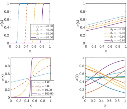
Figure 1: The functionsσiof (2.2) with varying parameters. On the top left panel, we have
setαi = 100, on the top right, αi = 1. On the bottom left functions with a fixed center
Ci= 1/2 are depicted. On the bottom right, a set of 10 functions obtained by varying the
coefficients as stated in Section 3.
output layer. The analysis reviewed in [22] gives the conditions that are re-quired for ensuring the interpolation property, thus the non-singularity of the collocation matrices; we report this result in Section 4.
OutsideIS, the functionσi is almost constant; then, we focus on the values of the parametersαi, βisuch that the intersection of the S–shape amplitudeIS and the domain of interest is non-null, thus leading to functionsσiwithCiinside the interval. The choice ofαi is related to the behavior of the derivative of the function. When taking all internal weightsαi ≡K, one obtains Heaviside-like functions ifK is big (as used in [16]), or almost-linear functions ifK is small (as used in [14, 30]). In our case, the use of both kind of functions can help to approximate both steep gradients and global behaviors. In figure 1, we plot different cases of such functions: on the top panels αi is a constant, on the bottom left panelCi is set equal to the mid-point of the interval and finally on
the bottom right panel, we plot functions with random values of αi, βi. Note that some functions can have similar shapes: interpolation properties are not changed but the problem can become ill-conditioned.
3. The proposed numerical algorithm
In this section, we propose a simple algorithm to get a numerical approxima-tion of a linear differential problem with the aid of ELM networks withnneurons in the hidden layer. The main idea is to fix the range of values of weights and biases, so that we construct a “good” basis ofnsigmoid functionsσi, and use a collocation method to fix the weights of the linear output activation function.
For our illustrations, we have chosen a stationary one-dimensional PDE with constant coefficients. −µu′′ (x) +γu′ (x) +λu(x) =f(x), x∈I:= [0,1]⊆R ν0u′(0) +ρ0u(0) =g0, ν1u′(1) +ρ1u(1) =g1, (3.1)
whereµ, γ and λare respectively the diffusion, advection and reaction terms. The domain is fixed to [0,1] for convenience. The boundary conditions are in the general Robin form; Dirichlet and Neumann boundary conditions are derived by settingνi= 0 orρi= 0.
Input: coefficientsµ, γ, λ;ν, ρ ; number of neuronsn, number of collocation pointsM, function evaluations [f,g]∈RM
1. setα∈Rn randomly according to (3.3) ;
2. setβ∈Rn such thatCi are uniformly distributed, i.e. βi=−αi∗Ci;
3. compute matrixS according to (3.5)-(3.6) ;
4. computeBaccording to (3.7)-(3.8) ;
5. solve the (eventually under/over -determined) linear system [S;B]w= [f;g] ;
Output: weights w∈Rn that fix the ELM approximate solution ˜u(x)
in (3.2);
We consider an approximate solution ˜u(x,w) given by the ELM: ˜ u(x;w) = n X i=1 wiσi(x). (3.2)
We choose α to be random uniformly distributed in a range that depends on the number of neurons n; if we fix the domain of the differential problem to have unitary length, we choose:
α:= rand −n−10 10 −4, n−10 10 + 4 . (3.3)
In this way, if n = 10 we have a maximum weight e.g. 4 and asn grows by 10 then the maximum weight grows by 1. The biases β are fixed so that the centersCi=−βi/αi of the sigmoid functions are located on random uniformly distributed points inside the interval.
Then, the ELM network is collocated in (3.1) onM−2 equidistant collocation pointsxj ∈(0,1) getting:
−µ˜u′′
(xj) +γu˜′(xj) +λ˜u(xj) =f(xj) forj= 2, . . . , M−1. (3.4)
Analytical derivatives of the sigmoid function σi can be computed by (2.3). Then: −µ n X i=1 wiσi′′(xj) +γ n X i=1 wiσ′i(xj) +λ n X i=1 wiσi(xj) =f(xj) forj= 2, . . . , M−1.
Finally, we observe that we can write separately the external weights w and write this in a matrix form as:
Sw:= (−µS(2)+γS(1)+λS(0))w=f, (3.5)
whereS2,S1 andS0 are matrices of elements:
S(2)= σ′′ i(xj) i,j , S(1)= σ′ i(xj) i,j andS(0) = σi(xj) i,j i= 1, . . . , n , j= 2, . . . , M−1 (3.6)
For the boundary conditions defined in (3.1), we augment the system by two equations collocating on the boundary points 0 and 1
ν n X i=1 wiσi′(xk) +ρ n X i=1 wiσi(xk) =g(xk) k= 0, M; x1= 0, xM = 1.
As before, we rewrite the above in a matrix form:
Bw:= (νB(1)+ρB(0))w=g, (3.7)
whereB(1) andB(0) are matrices of elements:
B(1)= σ′ i(xk) i,k andB(0) = σi(xk) i,k i= 1, . . . , n , k= 0, M . (3.8)
To this end, we have a linear system ofM equations andnunknowns. The over-all system can be constructed to be over-determined (M > n), under-determined (M < n) or squared (M = n). In the over- and under-determined cases, we consider the solution to be the one obtained in the least-square sense (in the under-determined problem the minimum-norm regularized solution). In the next section, we show that the under-determined solutions reach the same ac-curacy when compared with squared or over-determined cases. Moreover, we observe that the squared case can lead to ill-conditioned linear problems, so we propose under-determined collocation.
4. Analysis of the collocation approximation
In this section, building on previous works [5, 21, 25], we prove the consis-tency of the proposed ELM collocation method. First, based on the Theorem 2.1 presented in [25], we state the following Theorem that fits to our proposed framework.
Theorem 4.1. Let(xi, yi), i= 1, . . . , M be a set of points such thatxi< xi+1, and take the ELM network withn < M neuronsu(x;˜ w) in (3.2)such that the internal weightsαand the biasesβ are randomly generated independently from the data according to any continuous probability distribution. Then, ∀ε > 0, there exists a choice of w such that k(˜u(xi;w)−yi)ik< ε . Herek · k denotes the L2 Euclidean norm of vectors, the analogous of the Frobenius norm.
The above theorem states that if the number of hidden neurons are at least equal to the number of data points, then the interpolation error is zero. Start-ing from the above theorem, we consider the properties of ELM network for the approximation of functions. To do this, we consider the construction of a sequence of nested ELM families: E(n) := {u(x;˜ w), w ∈ Rn} ⊂ E(n+1) :=
{u(x;˜ w), w∈Rn+1}, where we add one neuron at time.
Based on the above theorem, we can now state the following theorem (see e.g. Theorem 2 of [22]).
Theorem 4.2. Let φ(x)be a continuous function. Then there exist a sequence of ELM network functionsu˜(n)∈E(n) such that:
kφ−u˜(n)kL2→0,
where byk · k2 we denote the L2 norm.
To prove the above, we consider a family of nested sets of ordered distinct points{x(iM), i= 1, . . . , M} ⊂ {x(iM+1), i= 1, . . . , M+ 1} and call diameter of the set of points H > 0 the maximum H = maxi=1,...,M−1(x(i+1M)−x
(M)
i ).
Then take in the space E(n) and call ˜u(n) the ELM network that interpolates
φon a set of points of diameterH: from Theorem 4.1 this construction exists. Finally, we can say that k(φ(xi)−u˜H(n)(xi))k →H→0 0, using the vector norm:
theorem 4.2 extends the convergence to a general continuous functionφin the L2sense, thus states that the finite-dimensional discrete space of ELM networks
is consistent in theL2setting.
Theorem 4.1 and 4.2 also imply that the collocation matricesS(0) are of full
rank.
We should note that for the problems that we consider here, in some cases we obtain ill-conditioned matrix problems. In these cases the solution of the under-determined collocation (number of neurons greater then number of points) with least squares is more suitable.
The collocation solution can now be sought as a solution of a variational formulation tested against delta-type functions or, equivalently, a discretized
formulation of the problem with C2 test functions. We follow the classic
ap-proach, see e.g. [5, 42] and write the weak formulation for the equation (3.1) that seeks au(x) in the trial space (denoted by U) such that:
Z 1
0
[−µu′′(x) +γu′(x) +λu(x)] v(x)dx=
Z 1
0
f(x)v(x)dx
for all test function v ∈ V. For simplicity, we suppose that the boundary conditions are imposed on the space U and are satisfied in all the subspaces introduced.
The general Galerkin method is a weak formulation as above where we look for a function ˜un ∈Un for which the equations hold true∀vm∈Vmand both Un andVm are finite-dimensional. In our case, we fixUn=E(n), i.e. the ELM
space with nneurons, so that the degrees of freedom of the finite dimensional space are the weightsw∈Rn.
Now, consider the test space to Vm =span{δi,ε(x), i= 1, . . . , m} defined
starting from a set ofm=ndistinct points {xi}. We also consider functionf to be approximated by its interpolant in the space of ELM, i.e. ˜f ≈f , f˜∈ E(n), f˜(xi) =f(xi). Then the Galerkin problem reads:
Z 1 0 [−µ˜u′′ ε(x) +γu˜ ′ ε(x) +λ˜uε(x)]δxi,ε(x)dx= Z 1 0 ˜ f(x)δxi,ε(x)dx ∀i= 1, . . . , M (4.1)
where functionsδare defined by
δxi,ε(x) =φ(|x−xi|/ε), φ(ζ) = exp{1/(ζ2−1)} R exp{1/(ζ2−1)}dζ ζ∈[0,1) 0 ζ∈[1,+∞) .
This Galerkin problem is related to the above collocation problem by the fol-lowing theorem.
Theorem 4.3. Let u˜n,ε(x) be a solution to the Galerkin problem (4.1). Then limε→0u˜n,ε(x) = ˜un(x) where u˜n(x) is the solution in the ELM space of the
collocation problem (3.4) on the points{xi}:
−µ˜u′′
This result follows from convergence of the integrals to evaluations of func-tion on sites, due to the convergence ofδ functions to δ distributions; a proof of this can be found in [5].
Based on the Theorem 2.2 presented in [42], we are now ready to prove the following convergence theorem for our proposed scheme.
Theorem 4.4. Let {x(in), i= 1, . . . , n}n∈Nbe an increasing family of colloca-tion points such that the diameterH tends to zero. Moreover takeE(n)a family of ELM. where we assume that matrix S of equation (3.5) constructed on the collocation points is full rank and uniformly invertible.
Then, if ˜un ∈ E(n) is ELM network solution to the collocation problem (4.2)
andu(x)is the solution to equation (3.1), we have that:
lim
n→∞k˜un−ukL
2= 0
Proof. Denote byLthe differential operator in equation (3.1), such thatLu=f. CallQn : φ∈Rn the operator that gives evaluation of function collocated on points {xi}, i.e. Qn(φ) = (φ(xi))i. Then call Pn : φ ∈ Rn the operator that gives the ELM network that interpolates functions at collocation nodes, i.e. Pn(φ) = ˜φ := Pwjσj(x) such that ˜φ(xi) = φ(xi). Then the solution ˜un to the collocation problem can be seen as the solution toQnLPnu˜n =Qnf, and matrixSof equation (3.5) is the discrete representation of the operatorQnLPn.
With this we have:
Lu=f ⇒QnLu=Qnf ⇒ QnLu−QnLPnu+QnLPnu=Qnf ⇒
QnLPnu+QnL(u−Pnu) =Qnf ⇒ u−(QnLPn)−1Qnf = (QnLPn)−1QnL(Pnu−u)
At last notice that fromQnLPnu˜n=Qnf we can write ˜un = (QnLPn)−1Qnf. Finally:
In this, we have that the first term is bounded from the hypothesis on the operatorS−1; the operatorQ
n is trivially bounded in our setting; the linearity of operatorLimply that also the third term is bounded. The thesis then follows from the convergence properties stated in theorems 4.1-4.2.
We remark that the collocation equations can be derived also via quadrature rules applied to equations (4.1). In this case there is no need of Theorem 4.3, and the relation with collocation is obtained by the requirement that the quadrature rule is supported on the collocation points. In this case, the functions δ can be substituted with any family of locally supported functions whose support includes only one collocation point.
5. Numerical results
In this section, we apply the proposed method for the solution of benchmark problems exhibiting steep gradients as suggested in [33]. More particularly, in Section 5.1, we first consider regular problems, in Section 5.2 boundary layer problems, and in Section 5.3 internal layer problems. For our computations, we have used Matlab2020b. In order to get reproducible results, we have used rng(5) to create the random values for the vectorsα,βbefore calling the random value generator of Matlab (rand). The solution of the least squares problems is achieved via the backslash command.
For each problem, the numbernof neurons ranged from 10 to 1280, doubling the number of neurons at each execution. For each fixedn, we compute solutions with various numbersM of collocation points. The computational time for all the above problems was of the order of 0.5 sec on a single intel core i7-10750H with 16GB RAM 2.60Ghz. In particular the maximum computational time was 0.6 sec forn= 1280. To evaluate the approximation error, we used two different metrics: the absolute difference between computed and exact solution, denoted byEu, and the residual of the equation, denoted byRf:
Eu(x) =|u(x)−u(x)˜ |
Note, that all errors are absolute, not normalized. Then, we computed theL2
norm of Eu and Rf; when computing the L2-norm, we used 5000 equispaced points and the trapezoidal rule for integration. As reference numerical method, we considered the finite difference (FD) scheme obtained with a maximal order on 7 nodes computed on M equispaced points. The FD function considered here is the piecewise linear polynomial one interpolating the computed values. We emphasize that in all computations the number of points considered for the FD solution is equal toM, i.e. the number of collocation equations considered for the ELM implementation. In two cases, we also considered the solution only at collocation points, thus consideringL∞ errors between vectors inRM.
5.1. Regular problems
In this section, we analyze sinusoidal-bump problems as well as a high-order polynomial problem to show that the proposed approach can result to a high approximation accuracy.
The first example is a simple 1D boundary value problem with homogeneous Dirichlet boundary conditions:
u′′+ (4k2π2−1)u= 4kπexcos(2kπx), 0< x <1 u(0) = 0, u(1) = 0 withk∈N
(5.1)
The above has the exact analytical solution:
u= exp(x) sin(2kπx)
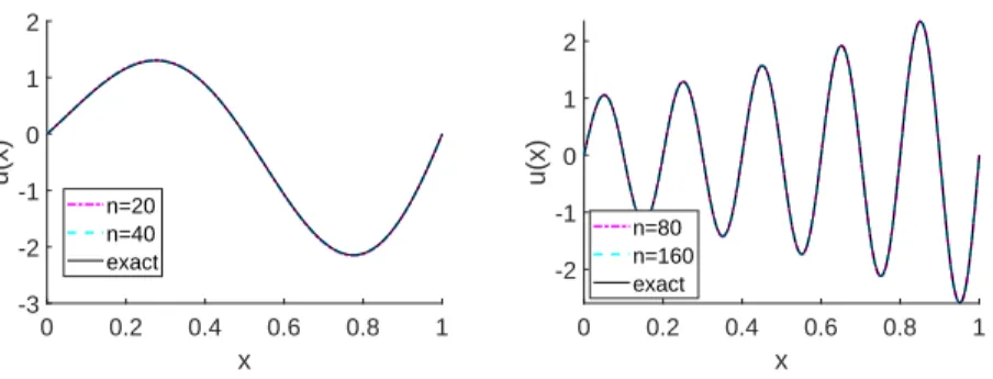
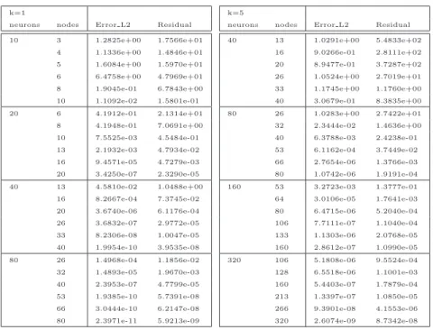
The coefficientk represents the number of oscillations in the domain. We con-sider the simple case with k = 1 and a more challenging one with k = 5 (see Figure 2. The computed errors with respect to the exact solution are reported in Figure 2 and in Table 1. In both cases, we note that the proposed ELM network results to a good approximation with a modest number of neurons.
0 0.2 0.4 0.6 0.8 1 x -3 -2 -1 0 1 2 u(x) n=20 n=40 exact 0 0.2 0.4 0.6 0.8 1 x -2 -1 0 1 2 u(x) n=80 n=160 exact
Figure 2: Applying the proposed ELM network for the numerical solution of the problem given in (5.1): approximation withnneurons, the number of collocation pointsM fixed to be
n/2 (on the left panel,k= 1, on the right panel,k= 5.)
containing a high-order polynomial:
u′′ = 22ppx(1−x)p−2xp−2(−1 + 2x−2x2+p(1−4x+ 4x2)), 0< x <1 u(0) = 0, u(1) = 0 (5.2) The above BV problem has the exact solution:
u(x) = 22pxp(1−x)p (5.3)
Here, we consider the casep= 10, so that to get a non-exact solution with FD. The computed errors arising from the proposed ELM network with respect to the exact analytical solution are reported in Figure 5.
5.2. Boundary Layer problems
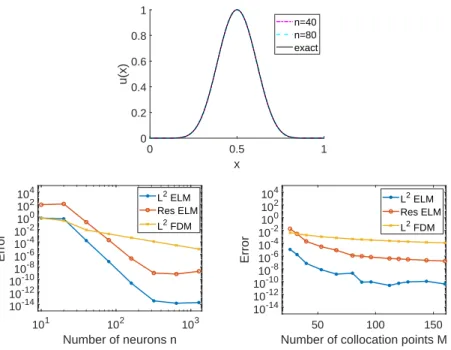
In this section, we consider benchmark boundary layer problems, namely an advection-dominated and a reaction-dominated problem that lead to sharp gradients near the boundary (see also [37]). We show how the proposed scheme can deal properly with the steep gradients that arise in these cases.
Whenλ= 0 andf ≡0 in (3.1), we have a diffusion-advection problem. If we impose Dirichlet boundary conditions withg0= 0, g1= 1, the solution reads:
u(x) = exp γ µx −1 exp γ µ −1 . (5.4)
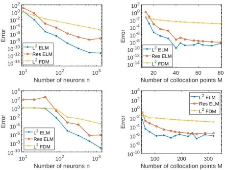
101 102 103 Number of neurons n 10-14 10-12 10-10 10-8 10-6 10-4 10-2 100 102 Error L2 ELM Res ELM L2 FDM 20 40 60 80 Number of collocation points M 10-14 10-12 10-10 10-8 10-6 10-4 10-2 100 102 Error L2 ELM Res ELM L2 FDM 101 102 103 Number of neurons n 10-10 10-8 10-6 10-4 10-2 100 102 104 Error L2 ELM Res ELM L2 FDM 100 200 300 Number of collocation points M 10-10 10-8 10-6 10-4 10-2 100 102 104 Error L2 ELM Res ELM L2 FDM
Figure 3: Error and residual convergence for the ELM numerical solution of the problem (5.1). On the top panels,k= 1: on the left top panelM=n/2, on the right top paneln= 40. On the bottom panels,k= 5: on the left bottom panel,M =n/2, on the right bottom panel,
n= 160.
If|γµ|<<1, the solution approaches the line connecting the boundary conditions while if|µγ|>>1 the solution is near to zero in almost the whole domain, except in a neighborhood of the right boundary where the function has a steep gradient. In this last case, we say that the solution has aboundary layer of width order
O µ
γ
. From a numerical point of view, for the particular problem, in which advection dominates diffusion, we need to catch the behavior on a small scale µ
γ, but it is well known that using finite difference or finite element methods, the approximate solution can oscillate while the exact solution is monotone (see [37]).
In the advection-dominated problem, the presence of the boundary layer is usually related to the so-called global P´eclet number:
Peg= |γ| · |I|
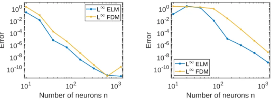
101 102 103 Number of neurons n 10-10 10-8 10-6 10-4 10-2 100 Error L ELM L FDM 101 102 103 Number of neurons n 10-10 10-8 10-6 10-4 10-2 100 Error L ELM L FDM
Figure 4: Converge plots of theL∞
norm at the collocation points for the solution of the problem (5.1): on the left panel,k= 1, on the right panel,k= 5.
where|I|is the domain length.
We considered the case with γ = 100 and µ = 1, with a P´eclet number
Peg= 50. Figure 5 depicts the exact analytical solution and some of the ELM
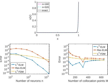
numerical solutions along with the corresponding approximation errors. When γ= 0,λ >0 andf ≡0 in the problem (3.1), we have a diffusion-reaction prob-lem. As before, we impose Dirichlet boundary conditions withg0= 0, g1= 1.
The problem has analogous difficulties as the previous one. The exact analytical solution is:
u(x) =sinh(θx)
sinh(θ), whereθ=
p
λ/µ. (5.6)
Also in this case the solution can give steep gradients ifλ/µ >>1. We call this behavior asboundary layer at the right boundary of width orderO(p
µ/λ). In this case, the usual definition of global P´eclet number is:
Peg=|λ| · |I|
2
6µ . (5.7)
We have setλ= 300 andµ= 1 so that the P´eclet number isPeg= 50 as before.
The computed errors with respect to the exact solution are reported in Figure 7.
Finally, we consider both the advection- and the reaction- dominated prob-lems taking different γ and λso that we get appropriate values of the P´eclet number. In Figure 8, we plot the L2 errors of the computed ELM solutions
k=1
neurons nodes Error L2 Residual 10 3 1.2825e+00 1.7566e+01 4 1.1336e+00 1.4846e+01 5 1.6084e+00 1.5970e+01 6 6.4758e+00 4.7969e+01 8 1.9045e-01 6.7843e+00 10 1.1092e-02 1.5801e-01 20 6 4.1912e-01 2.1314e+01 8 4.1948e-01 7.0691e+00 10 7.5525e-03 4.5484e-01 13 2.1932e-03 4.7934e-02 16 9.4571e-05 4.7279e-03 20 3.4250e-07 2.3290e-05 40 13 4.5810e-02 1.0488e+00 16 8.2667e-04 7.3745e-02 20 3.6740e-06 6.1176e-04 26 3.6832e-07 2.9772e-05 33 8.2306e-08 1.0047e-05 40 1.9954e-10 3.9535e-08 80 26 1.4968e-04 1.1856e-02 32 1.4893e-05 1.9670e-03 40 2.3953e-07 4.7799e-05 53 1.9385e-10 5.7391e-08 66 3.0444e-10 6.2147e-08 80 2.3971e-11 5.9213e-09 k=5
neurons nodes Error L2 Residual 40 13 1.0291e+00 5.4833e+02 16 9.0266e-01 2.8111e+02 20 8.9477e-01 3.7287e+02 26 1.0524e+00 2.7019e+01 33 1.1745e+00 1.1760e+00 40 3.0679e-01 8.3835e+00 80 26 1.0283e+00 2.7422e+01 32 2.3444e-02 1.4636e+00 40 6.3788e-03 2.4238e-01 53 6.1162e-04 3.7449e-02 66 2.7654e-06 1.3766e-03 80 1.0742e-06 1.9191e-04 160 53 3.2723e-03 1.3777e-01 64 3.0106e-05 1.7641e-03 80 6.4715e-06 5.2040e-04 106 7.7111e-07 1.1040e-04 133 1.1303e-06 2.0768e-05 160 2.8612e-07 1.0990e-05 320 106 5.1808e-06 9.5524e-04 128 6.5518e-06 1.1001e-03 160 5.4403e-07 1.7879e-04 213 1.3397e-07 1.0850e-05 266 9.3901e-08 4.1553e-06 320 2.6074e-09 8.7342e-08
Table 1: Error and residuals for the ELM numerical solution of problem (5.1): on the left table,k= 1, on the right tablek= 5.
5.3. Internal Layer Problems
In this section, we consider high transient problems that lead to an internal layer. For the solutions of these problems an adaptive mesh is usually proposed. For a description of the numerical problems that can arise, we refer to [33]. In this section, we show that the ELM network can provide good approximations. First, we consider theatanproblem:
−u′′= (2α3(x−x0) (1+α2(x−x 0)2)2, 0< x <1 u(0) =θ0, u(1) =θ1 (5.8)
θ0, θ1 are fixed in order to have an exact solution that reads:
u(x) = atan(α(x−x0)) (5.9)
In our tests, we fixα= 60 andx0= 4/9 that leads to a non-symmetric internal
0 0.5 1 x 0 0.2 0.4 0.6 0.8 1 u(x) n=40 n=80 exact 101 102 103 Number of neurons n 10-14 10-12 10-10 10-8 10-6 10-4 10-2 100 102 104 Error L2 ELM Res ELM L2 FDM 50 100 150 Number of collocation points M 10-14 10-12 10-10 10-8 10-6 10-4 10-2 100 102 104 Error L2 ELM Res ELM L2 FDM
Figure 5: Numerical tests for the solution of problem (5.2) withp= 10. On the top panel are depicted the exact (5.3) and the ELM numerical solutions withn= 40,80; the number of collocation pointsMwas set ton/2. On the bottom panels are shown the error and residual convergence: on the left panel, we fixM = n/2 and vary nand on the right panel we fix
n= 80 and varyM
.
numerical ones. The approximation errors with respect to the exact-analytical solution are also given.
The second test with internal peak is a rescaled sinusoidal problem suggested in [39]: −u′′= −4x2 ε2 + 2 ε e−x2 /ε, 0< x <1 u(0) =θ0, u(1) =θ1 (5.10)
θ0, θ1 are fixed in order to have as exact solution:
u(x) =e−x2
/ε . (5.11)
We consider the caseε= 10−3. Figure 10 depicts the exact-analytical solution
and some of the numerical ones. The approximation errors with respect to the exact-analytical solution are also given.
0 0.5 1 x 0 0.2 0.4 0.6 0.8 1 u(x) n=160 n=320 exact 101 102 103 Number of neurons n 10-10 10-8 10-6 10-4 10-2 100 102 104 Error L2 ELM Res ELM L2 FDM 200 400 600 Number of collocation points M 10-10 10-8 10-6 10-4 10-2 100 102 104 Error L2 ELM Res ELM L2 FDM
Figure 6: Numerical tests for the solution of the problem (3.1) withµ= 1, γ= 100, λ= 0. In this case, the P´eclet number isPeg= 50, the boundary layer is of the order of 10−2. On the
top panel are shown both the exact (5.4) and the ELM numerical solutions withn= 40,80; the number of collocation points isM=n/2. On the bottom panels are shown the error and residual convergence plots; on the left panel we fixM =n/2 and varynand on the right panel we fixn= 320 and varyM.
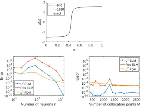
To this end, we consider a very difficult numerical problem that has as exact-analytical solution a comb-like profile. For this problem, we compute the approximation errors using several number of neurons and the behavior only on collocation points. The equation we consider is the following:
−u′′=−2(ε+x) cos 1 ε+x −sin 1 ε+x (ε+x)4 , 0< x <1 u(0) =θ0, u(1) =θ1 (5.12)
We have setθ0, θ1in order to have the following exact-analytical solution:
u(x) = sin 1 ε+x
!
. (5.13)
Then, we considered the case ε = 1/10π that gives a solutions with 10 zeros and 5 oscillations in the domain. Figure 11 depicts the exact-analytical solution
0 0.5 1 x 0 0.2 0.4 0.6 0.8 1 u(x) n=40 n=80 exact 102 Number of neurons n 10-10 10-8 10-6 10-4 10-2 100 102 104 Error L2 ELM Res ELM L2 FDM 50 100 150 Number of collocation points M 10-10 10-8 10-6 10-4 10-2 100 102 104 Error L2 ELM Res ELM L2 FDM
Figure 7: Numerical tests for the solution of the problem (3.1) withµ= 1, γ= 0, λ= 300. In this case, the P´eclet number isPeg= 50, the boundary layer is of the order of 10−1. On the
top panel are shown the exact analytical (5.6) and the ELM numerical solutions forn= 40,80; the number of collocation points was set toM=n/2. On the bottom panels are depicted the error and the residual convergence: on the left panel we fixM=n/2 and varynand on the right panel we fixn= 80 and varyM.
as well as the ELM numerical solution for n = 1280,2560 and the resulting approximation errors with respect to the exact-analytical solution considering only the approximation errors at the collocation points using theL∞norm.
6. Conclusions and future work
In the present paper, we address collocation scheme based on ELM networks for the numerical approximation of 1D elliptic problems with steep gradients. The weights between the input layer and the hidden layer as well as the biases are fixed appropriately in advance and kept fixed. In this way, the only coefficients that describe the approximation space are the weights of the linear combination used for the element of the linear activation of the ELM. First, we have explored
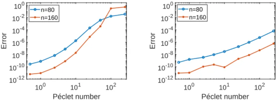
100 101 102 Péclet number 10-12 10-10 10-8 10-6 10-4 10-2 100 Error n=80 n=160 100 101 102 Péclet number 10-12 10-10 10-8 10-6 10-4 10-2 100 Error n=80 n=160 Figure 8: L2
errors of computed ELM solutions with fixednandM =n/2. On abscissae, we report the P´eclet number as computed with equation (5.5) on the left and equation (5.7) on the right. In particular, on the left panel we considerγ= [0,1,2,5,10,20,50,100,200,500] and on the right panelλ= [0,3,6,15,30,60,150,300,600,1500].
the underlying space, so as to construct it in a random but proper way. Then, the numerical solution to the boundary value problems was reduced to the computation of thenweights of the ELM network viaM collocation equations. We have proved the convergence of the scheme in the square case, and proposed the use of an underdetermined collocation scheme to avoid ill-conditioning.
Numerical tests were performed for the evaluation of the approximation accuracy of the proposed method with the aid of benchmark boundary value problems exhibiting sharp gradients. We also compared the proposed approach with a high order finite difference (FD) scheme. We show that for both internal and boundary layer problems the proposed method outperforms FD, when the number of neurons is taken to be big enough to catch the steep gradient of the layer. We emphasize also that in our case, the solutions areC∞ functions.
The proposed method can be further developed by exploring some alterna-tives, such as the use of optimal activation functions, as proposed in [14], or the selection of the solution of the under-determined system by using the properties of null rules, as explored in [7]. Finally, the application of the proposed ELM collocation method can be extended in various ways. Among others, we are currently considering the use for:
0 0.2 0.4 0.6 0.8 1 x -2 -1 0 1 2 u(x) n=640 n=1280 exact 101 102 103 Number of neurons n 10-10 10-8 10-6 10-4 10-2 100 102 104 106 Error L2 ELM Res ELM L2 FDM 500 1000 1500 2000 2500 Number of collocation points M 10-10 10-8 10-6 10-4 10-2 100 102 104 106 Error L2 ELM Res ELM L2 FDM
Figure 9: Numerical tests for the solution of problem (5.8) withα= 60 andx0= 4/9. On the top panel it is depicted the exact-analytical (5.9) and the ELM numerical solutions for
n= 640,1280; the number of collocation pointsM was fixed ton/2. On the bottom panel, we depict the error and residual convergence: on the left panel, we fixM =n/2 and varyn
and on the right panel we fixn= 1280 and varyM.
• Multidimensional problems;
• Time-dependent problems;
• Inverse problems with overfitting.
Acknowledgements
The authors would like to thank Prof. Ferdinando Auricchio, Prof. Bert J¨uttler for fruitful discussions on the subject of the paper. Francesco Calabr`o are partially supported by INdAM, through GNCS research projects. This support is gratefully acknowledged.
-1 -0.5 0 0.5 1 x 0 0.2 0.4 0.6 0.8 1 u(x) n=640 n=1280 exact 101 102 103 Number of neurons n 10-12 10-10 10-8 10-6 10-4 10-2 100 102 104 106 Error L2 ELM Res ELM L2 FDM 500 1000 1500 2000 2500 Number of collocation points M 10-12 10-10 10-8 10-6 10-4 10-2 100 102 104 106 Error L2 ELM Res ELM L2 FDM
Figure 10: Numerical results for the solution of the problem (5.10) withε= 10−3
. On the top panel are depicted the exact-analytical (5.11) and the computed ELM solutions with number of neuronsn= 640,1280 and number of collocation pointsM =n/2. On the bottom panel, are depicted the error and residual convergence: on the left panel, we fixM =n/2 and vary
nand on the right panel, we fixn= 1280 and varyM.
References
[1] J. Almira, P. Lopez-de Teruel, D. Romero-Lopez, and F. Voigtlaender. Neg-ative results for approximation using single layer and multilayer feedforward neural networks. Journal of Mathematical Analysis and Applications, page 124584, 2020.
[2] C. Anitescu, E. Atroshchenko, N. Alajlan, and T. Rabczuk. Artificial neural network methods for the solution of second order boundary value problems.
Computers, Materials and Continua, 59(1):345–359, 2019.
[3] H. Arbabi, J. E. Bunder, G. Samaey, A. J. Roberts, and I. G. Kevrekidis. Linking machine learning with multiscale numerics: Data-driven discovery of homogenized equations. JOM, pages 1–14, 2020.
0 0.5 1 x -1.5 -1 -0.5 0 0.5 1 1.5 u(x) n=1280 n=2560 exact 101 102 103 Number of neurons n 10-4 10-2 100 102 104 106 Error L2 ELM Res ELM L2 FDM 101 102 103 Number of neurons n 10-4 10-2 100 102 104 106 Error L ELM L FDM
Figure 11: Numerical results for the solution of the problem (5.12) with ε= 1/10π. On the top panels it is depicted the exact-analytical (5.13) and the numerical solutions with the number of neuronsn= 1280,2560 and number of collocation points fixed atM =n/2. On the bottom panels are shown the error and residual convergence: on the left panel, it is shown the
L2
norms with fixedM=n/2 and on the right panel it is shown theL∞
on the collocation points.
[4] J.-G. Attali and G. Pag`es. Approximations of functions by a multilayer perceptron: a new approach. Neural networks, 10(6):1069–1081, 1997.
[5] F. Auricchio, L. B. Da Veiga, T. J. Hughes, A. Reali, and G. Sangalli. Isogeometric collocation for elastostatics and explicit dynamics. Computer methods in applied mechanics and engineering, 249:2–14, 2012.
[6] J. Berg and K. Nystr¨om. A unified deep artificial neural network approach to partial differential equations in complex geometries. Neurocomputing, 317:28–41, 2018.
[7] F. Calabr`o, D. Bravo, C. Carissimo, E. Di Fazio, A. Di Pasquale, A. Eldray, C. Fabrizi, J. Gerges, S. Palazzo, and J. Wassef. Null rules for the detection
of lower regularity of functions. Journal of Computational and Applied Mathematics, 361:547–553, 2019.
[8] Q. Chan-Wai-Nam, J. Mikael, and X. Warin. Machine learning for semi linear pdes. Journal of Scientific Computing, 79(3):1667–1712, 2019.
[9] D. Costarelli and R. Spigler. Approximation results for neural network operators activated by sigmoidal functions. Neural Networks, 44:101–106, 2013.
[10] G. Cybenko. Approximation by superpositions of a sigmoidal function.
Mathematics of control, signals and systems, 2(4):303–314, 1989.
[11] C. De Falco and E. O’Riordan. Interior layers in a reaction-diffusion equa-tion with a discontinuous diffusion coefficient. Int. J. Numer. Anal. Model, 7(3):444–461, 2010.
[12] L. Demkowicz, W. Rachowicz, and P. Devloo. A fully automatic hp-adaptivity. Journal of Scientific Computing, 17(1-4):117–142, 2002.
[13] V. Dwivedi and B. Srinivasan. Physics informed extreme learning machine (PIELM) - A rapid method for the numerical solution of partial differential equations. Neurocomputing, 391:96 – 118, 2020.
[14] N. J. Guliyev and V. E. Ismailov. On the approximation by single hidden layer feedforward neural networks with fixed weights. Neural Networks, 98:296–304, 2018.
[15] H. Guo, X. Zhuang, X. Meng, and T. Rabczuk. Analysis of three dimen-sional potential problems in non-homogeneous media with deep learning based collocation method. arXiv preprint arXiv:2010.12060, 2020.
[16] N. Hahm and B. I. Hong. An approximation by neural networks with a fixed weight. Computers & Mathematics with Applications, 47(12):1897– 1903, 2004.
[17] J. Han, A. Jentzen, and E. Weinan. Solving high-dimensional partial differ-ential equations using deep learning. Proceedings of the National Academy of Sciences, 115(34):8505–8510, 2018.
[18] J. Han, M. Nica, and A. R. Stinchcombe. A derivative-free method for solving elliptic partial differential equations with deep neural networks.
Journal of Computational Physics, 419:109672, 2020.
[19] K. Hornik, M. Stinchcombe, and H. White. Universal approximation of an unknown mapping and its derivatives using multilayer feedforward net-works. Neural networks, 3(5):551–560, 1990.
[20] K. Hornik, M. Stinchcombe, H. White, et al. Multilayer feedforward net-works are universal approximators. Neural networks, 2(5):359–366, 1989.
[21] H.-Y. Hu and Z.-C. Li. Collocation methods for Poisson’s equation. Com-puter Methods in Applied Mechanics and Engineering, 195(33-36):4139– 4160, 2006.
[22] G. Huang, G.-B. Huang, S. Song, and K. You. Trends in extreme learning machines: A review. Neural Networks, 61:32 – 48, 2015.
[23] G.-B. Huang, D. H. Wang, and Y. Lan. Extreme learning machines: a sur-vey. International journal of machine learning and cybernetics, 2(2):107– 122, 2011.
[24] G.-B. Huang, Q.-Y. Zhu, and C.-K. Siew. Extreme learning machine: a new learning scheme of feedforward neural networks. In2004 IEEE inter-national joint conference on neural networks (IEEE Cat. No. 04CH37541), volume 2, pages 985–990. IEEE, 2004.
[25] G.-B. Huang, Q.-Y. Zhu, and C.-K. Siew. Extreme learning machine: the-ory and applications. Neurocomputing, 70(1-3):489–501, 2006.
[26] Y. Ito. Nonlinearity creates linear independence. Advances in Computa-tional Mathematics, 5(1):189–203, 1996.
[27] I. E. Lagaris, A. Likas, and D. I. Fotiadis. Artificial neural networks for solving ordinary and partial differential equations. IEEE transactions on neural networks, 9(5):987–1000, 1998.
[28] I. E. Lagaris, A. C. Likas, and D. G. Papageorgiou. Neural-network meth-ods for boundary value problems with irregular boundaries. IEEE Trans-actions on Neural Networks, 11(5):1041–1049, 2000.
[29] S. Lee, M. Kooshkbaghi, K. Spiliotis, C. I. Siettos, and I. G. Kevrekidis. Coarse-scale pdes from fine-scale observations via machine learning.Chaos: An Interdisciplinary Journal of Nonlinear Science, 30(1):013141, 2020.
[30] S. Lin, X. Guo, F. Cao, and Z. Xu. Approximation by neural networks with scattered data. Applied Mathematics and Computation, 224:29–35, 2013.
[31] L. Lu, X. Meng, Z. Mao, and G. E. Karniadakis. Deepxde: A deep learning library for solving differential equations. arXiv preprint arXiv:1907.04502, 2019.
[32] C. Michoski, M. Milosavljevi´c, T. Oliver, and D. Hatch. Solving differential equations using deep neural networks. Neurocomputing, 2020.
[33] W. F. Mitchell. A collection of 2D elliptic problems for testing adaptive grid refinement algorithms. Applied Mathematics and Computation, 220:350 – 364, 2013.
[34] E. O˜nate, J. Miquel, and P. Nadukandi. An accurate FIC-FEM formulation for the 1D advection–diffusion–reaction equation. Computer Methods in Applied Mechanics and Engineering, 298:373–406, 2016.
[35] G. Pang, L. Yang, and G. E. Karniadakis. Neural-net-induced gaussian process regression for function approximation and pde solution. Journal of Computational Physics, 384:270–288, 2019.
[36] A. Pinkus. Approximation theory of the MLP model in neural networks.
[37] A. Quarteroni. Diffusion-transport-reaction equations. InNumerical Mod-els for Differential Problems, pages 315–365. Springer, 2017.
[38] K. Rudd and S. Ferrari. A constrained integration (CINT) approach to solving partial differential equations using artificial neural networks. Neu-rocomputing, 155:277–285, 2015.
[39] A. Schmidt and K. G. Siebert. A posteriori estimators for the h–p version of the finite element method in 1d. Applied numerical mathematics, 35(1):43– 66, 2000.
[40] J. Sirignano, J. F. MacArt, and J. B. Freund. DPM: A deep learning PDE augmentation method with application to large-eddy simulation. Journal of Computational Physics, 423:109811, 2020.
[41] J. Sirignano and K. Spiliopoulos. DGM: A deep learning algorithm for solving partial differential equations. Journal of Computational Physics, 375:1339–1364, 2018.
[42] G. Strang and G. J. Fix.An analysis of the finite element method. Prentice-hall, 1973.