A TIME-OPTIMAL ALGORITHM FOR THE ESTIMATION OF CONTACT DISTRIBUTION FUNCTIONS OF RANDOM SETS

(1)

A TIME-OPTIMAL ALGORITHM FOR THE ESTIMATION

OF CONTACT DISTRIBUTION FUNCTIONS OF RANDOM SETS

J

OHANNES

M

AYER

Department of Applied Information Processing and Department of Stochastics, University of Ulm, D-89069 Ulm, Germany

e-mail: [email protected]

(Accepted June 18, 2004)

ABSTRACT

This paper presents a linear-time and therefore time-optimal algorithm for the estimation of distance distribution functions and contact distribution functions of random sets. The distance distribution function is the area fraction of a dilated set, where this function depends on the size of the structuring element used for the dilation. Furthermore, contact distribution functions are related to distance distribution functions. Minus-sampling estimators are used for the estimation.

Keywords: algorithm, contact distribution, distance distribution, estimation, estimator, minus-sampling.

INTRODUCTION

Random sets, i.e., random variables whose values are sets, have successfully been applied to model patterns in various fields, such as materials science

(Ohser and M¨ucklich, 2000), medicine (Mattfeldt et

al., 1996), physics (Mecke, 1998), and astrophysics (Mecke et al., 1994). In their statistical analysis, so-called contact distribution functions (cdf’s) are very important,cf.Serra (1982); Stoyanet al.(1995); Ohser and M¨ucklich (2000). For a stationary random closed set Ξ, the spherical contact distribution function is the distribution function of the random (minimum

Euclidean) distance of an arbitrary point x outside

of Ξ to (the closest point at the boundary ∂Ξ

of) Ξ. The Euclidean metric yields the spherical

contact distribution function. Using other metrics, such as the city-block metric, yields further important contact distribution functions. There are various estimators for contact distribution functions,cf.Stoyan

et al. (1995). The classical estimators are

minus-sampling estimators. Stoyan et al. (2001) point

out that these estimators for cdf’s are as good as the more sophisticated estimators concerning the mean squared error. Therefore, the classical (minus-sampling) estimators are used in the following.

The cdf can be expressed in terms of the area fraction of the stationary random closed set dilated by a structuring element with variable size. In case of the spherical cdf, the structuring element is the unit-sphere.

When working with real data, binary images,

i.e., digital images with two phases, are the usual basis for the estimation. They can be interpreted as

discretized samples of random sets. Thus, the minus-sampling estimators have to be formulated for this case. This is not difficult. However, it turns out, that the running time of algorithms computing these estimators is usually not linear in the number of pixels of the image, but somewhat in between linear and quadratic – even when a distance transform is used and computed in linear-time. The presented novel algorithm additionally uses an efficient data structure to compute the minus-sampling estimator in linear time. In the following, the two-dimensional case is covered. However, the results can be generalized analogously to higher dimensions (with not much difficulty).

PRELIMINARIES

Let A and B be two arbitrary subsets of R2. By

Ac _:₌_{_x_∈_R2 _:_x_∈_/ _A_} _the _complement _{of the set} _A

is denoted. Letc be a real constant. ThencA:=_{cx:

x∈A}is thescalar multiplicationofcandA. The set

A⊕B:=_{x+y:x_∈A,y_∈B_}is called theMinkowski

addition of A and B. The Minkowski subtraction of

B from A is defined as AªB:= (Ac_⊕B)c. The set

B is called thestructuring element in the Minkowski addition and subtraction above. A structuring element

Bmcan be defined using a normmasBm:={x∈R2: m(x)_≤1_}. The discb(o,r) with radius r around the

origin is, thus, equal to the setrBmE, wheremE denotes

the Euclidean norm. (Note that each normm(_·)has an

associated metricd(x,y):=m(x₋y).)

LetX be a set from the extended convex ring over

R2. ThenA(X)denotes thearea. LetΞbe a stationary

(2)

W be a non-empty, bounded convex set, the so-called

sampling window.Ξ∩W is the random setΞobserved

within the sampling windowW. The specific area or

area fractionofΞis defined as

AA(Ξ):= E[A_A(Ξ∩W)]

(W) . (1)

Letxbe a (fixed) arbitrary point ofR2. ThenAA(Ξ) =

P(o_∈Ξ) =P(x_∈Ξ) holds. Thus,AcA(Ξ) = Ξ(x) is

a simple and unbiased estimator for AA(Ξ). Given a

finite set of pointsGofR2, an improved estimator for

the area fraction is given by AcA(Ξ) = _#1_G∑x∈G Ξ(x)

which is also unbiased and known as thepoint count

method. (#G denotes the cardinality of the set G.)G

can be seen as the vertices of a grid – the locations of the pixels of a binary image – and Ξ(x)can be seen

as the values of the pixels of a binary image. Thus, the previous estimator can easily be used for samples ofΞ

given as a binary image.

The area fraction can be studied for so-called

parallel sets Ξ⊕rB of Ξ, where B is a compact

and convex subset of R2. This yields the following

morphological function, where this function depends on the sizerof the structuring elementB:

AA(r):=AA(Ξ⊕rB) (2)

AA(r) is sometimes called the distance distribution

function. A normalized version of AA(r) is the

so-called contact distribution function HB₍_r₎ _{which can}

be defined as

HB₍_r₎_:₌₁₋1−AA(r)

1−AA(0) (3)

forr≥0. For example, choosingB=b(o,1)yields the

well-known spherical contact distribution function, denotedHs₍_r₎_.

LetB=Bm for some normm. Then, AA(r) is the

distribution function of the random (minimal) distance

between an arbitrarily chosen point x ∈R2 and Ξ.

Furthermore, HB₍_r₎ _{is the distribution function of}

the random (minimal) distance between an arbitrarily chosen pointx∈ΞcandΞ.

LetG be a finite grid overR2. Given a metricd,

thedistance transformof the setX onGis defined as

DX_d(x):=min_{d(x,y):y_∈G_∩Xc_} (4)

for eachx∈G. It associates each point with its minimal

distance to Xc _{(on the grid) – a different distance in}

comparison to the distance distribution and the contact distribution. For a binary image being a discretization of the set X on a rectangular grid G, this transform

can be computed in linear time (in the number of pixels) for various metrics, such as the Euclidean, the city-block, the maximum, etc., cf.Rosenfeld and Pfaltz (1966; 1968); Danielsson (1980); Soille (1991); Vincent (1991); Ragnemalm (1993); Breu (1995).

SOME ESTIMATION ALGORITHMS FOR DISTANCE DISTRIBUTION FUNCTIONS

As before, letΞbe a stationary random closed set over the extended convex ring,Ba compact and convex

subset of R2, and W a non-empty, bounded convex

set, namely the sampling window. A minus-sampling estimator for the distance distribution function is the following:

c

AA(r) = A([(Ξ∩W_A)₍⊕_WrB]∩(WªrB))

ªrB) (5)

for r ≥ 0 such that A(W _ªrB) > 0. Edge-effects

are removed through the reduction of the sampling

window fromWtoWªrB.

Let Gbe a finite rectangular grid overR2 for the

discretization ofΞandW. The area of the unit cell of

Gis calledA0. Furthermore, letB=Bmfor some norm

mand letdbe the metric associated withm. Then, the above estimator can be discretized as

f

AA(r) = A0∑x∈G [0,r]

(DΞ_dc(x))_· ₍_r_,∞_](DW d (x))

A0∑x∈G (r,∞](DW_d (x))

= ∑x∈G [0,r](D Ξc

d (x))· (r,∞](DW_d (x))

∑x∈G (r,∞](DW_d (x))

(6)

for r≥0 such that the denominator does not vanish. Informally speaking, this estimator gives the fraction of all pixels with (minimal) distance greater than r

to the boundary of the sampling windowW that have

(minimal) distance at mostrtoΞ.

The direct algorithm

The direct algorithm to compute the above discretized estimator first computes the distance transforms of Ξc _and _W _{(in linear time). (Note that}

the distance transform ofW can easily be computed

directly if W is a rectangle.) Thereafter, it computes the above fraction for each value ofr.

To make the description of the direct algorithm precise, the following listing is an implementation of this algorithm in Java. However, an implementation in C, C++, or C# would look very similar. For simplicity considerations, the images are represented by two-dimensional arrays. The complementation of a binary

image is done by the method C() and the distance

transform is computed by the method DT(). These

(3)

1float[] estimateDirect(boolean[][] im,

2 boolean[][] sw, int metric) 3{

4 // width and height of im and sw 5 int width = im.length;

6 int height = im[0].length; 7

8 // distance transform of sw 9 // and the complement of im

10 float[][] dim = DT(C(im), metric);

11 float[][] dsw = DT(sw, metric); 12

13 // arrays for numerator and denominator 14 int min = Math.min((width+1)/2,

15 (height+1)/2);

16 int[] num = new int[min]; 17 int[] denom = new int[min];

18 for (int r = 0; r < min; r++) 19 num[r] = denom[r] = 0;

20

21 // process each pixel for all values of r

22 for (int r = 0; r < min; r++)

23 for (int y = 0; y < height; y++) 24 for (int x = 0; x < width; x++) { 25 // increment denominator

26 if (r < dsw[x][y])

27 denom[r]++;

28

29 // increment numerator

30 if (r >= dim[x][y]

31 && r < dsw[x][y])

32 num[r]++;

33 }

34

35 // compute the estimator for all r

36 // such that denom[r] != 0 37 for (int r = 0; r < min; r++)

38 num[r] = (denom[r] == 0)

39 ? Float.NaN

40 : (float) num[r]

41 / (float) denom[r];

42

43 return num; 44}

The parameter imis a discretization of a sample

of Ξ and the parameter sw is a discretization of W,

i.e., imandsw are binary images. It is assumed that both have the same size (computed in lines 5 and

6). The parameter metric is passed to the method

that computes the distance transform. It determines the structuring elementBm. The numerator of the estimator

is stored in the arraynum; the denominator is stored

in the array denom. For values of r such that the

denominator of the estimator vanishes, the estimator is set to “not a number” (Float.NaN), since it cannot be determined in this case.

The computation of the fraction for one value ofr

takesΘ(#G) time and there areΘ(√#G) values of r

(if the image is quadratic). Thus, the direct algorithm has in each case time-complexity Θ(#G√#G). This is much more than linear time,i.e.,Θ(#G). Consider,

for example, a 1000×1000 pixels image, i.e., #G=

106_{. Then, #}_G√_#_G₌₁₀9 _{is significantly more than}

just #G.

An improved algorithm

The direct algorithm processed the image once for

each value of r. An obvious improvement is, thus,

to process the image only once and to compute for each pixel the range within which it is counted in the numerator resp. the denominator. Using an array for the numerator and the denominator, the elements of this array have to be initialized with zero at the beginning and incremented by one in the computed range for each pixel.

The following Java implementation makes the informal description of the improved algorithm precise:

1float[] estimateImproved(boolean[][] im, 2 boolean[][] sw, int metric)

3{

10 float[][] dim = DT(C(im), metric); 11 float[][] dsw = DT(sw, metric); 12

13 // arrays for numerator and denominator 14 int min = Math.min((width+1)/2,

15 (height+1)/2);

16 int[] num = new int[min];

17 int[] denom = new int[min]; 18 for (int r = 0; r < min; r++) 19 num[r] = denom[r] = 0; 20

21 // process all pixels

22 for (int y = 0; y < height; y++) 23 for (int x = 0; x < width; x++) {

24 float d_xi = dim[x][y];

25 float d_wc = dsw[x][y];

26 d_xi = Math.min(d_xi, d_wc); 27

28 // increment denominator

29 for (int r = 0; r < d_xi; r++)

30 denom[r]++;

31

32 // increment numerator

33 // and denominator

34 for (int r = d_xi; r < d_wc; r++) {

35 num[r]++;

36 denom[r]++;

(4)

38 } 39

40 // compute the estimator for all r 41 // such that denom[r] != 0

42 for (int r = 0; r < min; r++)

43 num[r] = (denom[r] == 0)

44 ? Float.NaN

45 : (float) num[r]

47

48 return num;

49}

It is interesting to study, how many increments are necessary for all pixels together. This yields the amortised time complexity of this algorithm. The number of all increments is obviously between once and twice the number of increments of the denominator. Thus, only the number of increments of the denominator is studied. For simplicity considerations let the sampling window be quadratic with even edge length n. If the distance of a pixel to

Wc_is_d_{, this leads to}_d_{increments of the denominator.}

It is easily verified that there are 4(2k)₋4 pixels with

distance n₂−k+1 to Wc for k =1, . . . ,n₂. Thus, the

total number of increments of the denominator is in each case

n/2

∑

k=1

(4(2k)₋4)³n

2−k+1

´

= n

3₊₃_n2₊₂_n

6 =Θ(n3) =Θ(#G

√

#G), (7)

with n=√#G. Thus, this algorithm also has

time-complexityΘ(#G√#G)in each case. The novel algorithm

The problem of the improved algorithm is that in each case Θ(√#G) increments are necessary for a

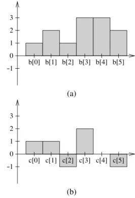
huge subset of the pixels. However, these increments are done within a continuous range of array elements. Now, the novel algorithm uses the improved algorithm, but it has a more sophisticated data structure to represent the numerator and the denominator than just a simple array. The basic requirement for this data structure is that only a constant number of increments (and decrements) is necessary to increment a whole (continuous) range (with the same value). Figure 1 shows two different representations of the same integer sequence(1,2,1,3,3,2).

0 1 3

−1 2

b[0] b[1] b[2] b[3] b[4] b[5]

(a)

0 1 3

−1 2

c[0] c[1] c[2] c[3] c[4] c[5]

(b)

Fig. 1.Two array representations of the same integer sequence.

(a) shows the direct representation of the sequence. In (b), the first element of the sequence and the differences to the previous element are stored, i.e.,

c[i] =b[i]₋b[i₋1]fori>0 andc[0] =b[0]. The array

bcan, thus, easily be restored fromcas follows:

b[0] =c[0] and b[i] =b[i₋1] +c[i], (8)

fori>0. To increment the elements of the sequence

in the range [n,n+m₋1] it takes m increments

in representation (a) and only two increments resp. decrements in representation (b), namely an increment ofc[n]and a decrement ofc[n+m]. Therefore, during

the processing of the pixels, the numerator and the denominator should be stored using representation (b). At the end, this representation is converted to the representation (a).

The following Java implementation gives a precise description of the novel algorithm:

1float[] estimateNovel(boolean[][] im, 2 boolean[][] sw, int metric) 3{

(5)

13 // arrays for numerator and denominator 14 // in representation (b)

15 int min = Math.min((width+1)/2,

16 (height+1)/2);

17 int[] num = new int[min];

18 int[] denom = new int[min]; 19 for (int r = 0; r < min; r++)

20 num[r] = denom[r] = 0; 21

22 // process all pixels

23 for (int y = 0; y < height; y++)

24 for (int x = 0; x < width; x++) {

25 float d_xi = dim[x][y];

26 float d_wc = dsw[x][y];

27

28 // increment denominator

29 if (d_wc > 0)

30 denom[d_wc-1]++;

31

32 // increment numerator 33 if (d_xi < d_wc) {

34 num[d_xi]++;

35 num[d_wc]--;

36 }

37 }

38

39 // reconstruct representation (a)

40 // in num and denom

41 for (int r = 1; r < min; r++) 42 num[r] += num[r-1];

43 for (int r = min-1; r > 0; r--) 44 denom[r-1] += denom[r];

45

46 // compute the estimator for all r

47 // such that denom[r] != 0 48 for (int r = 0; r < min; r++) 49 num[r] = (denom[r] == 0)

50 ? Float.NaN

51 : (float) num[r]

53

54 return num; 55}

The numerator of the estimator is stored in

the array num according to representation (b). The

denominator is stored in the array denom slightly

different; it contains the changes from right to left and not from left to right. All pixels are processed in the

lines 23–37. For each pixel, d_xi is its (minimal)

distance toΞandd_wcis its (minimal) distance toWc_;

cf.lines 25–26. The numerator has to be incremented in the range [d_xi, . . . ,d_wc−1], which requires

one increment and one decrement; cf. lines 33–36.

Analogously, the denominator has to be incremented in the range [0, . . . ,d_wc−1]. Thus, at most one

increment is necessary, since the changes are stored from right to left; cf. lines 29–30. After the integer sequences for the numerator and the denominator have been reconstructed in the lines 41–44, the estimator

can be computed in the lines 48–52.

Concluding, the time-complexity of the novel

algorithm is in each case Θ(#G), where #G is

the number of pixels of the image. Therefore, this algorithm is time-optimal, because linear time is the best possible case.

EMPIRICAL STUDY

So far, “only” asymptotical results have been presented. They show that the novel algorithm is at least of theoretical importance. But the constants hidden in theΘ-notation may be so huge that the novel algorithm could be of no practical importance.

For this reason, the (stationary) Boolean model with discs of radius 10 pixels and given hypothetical area fractionp∈ {0.1,0.2, . . . ,0.9_}has been simulated

for quadratic sampling windows of sizes (i.e., edge lengths) 512, 1024, 2048, and 4096 pixels. Samples of such Boolean models are shown in Figure 2.

The experiments have been conducted on an AMD Athlon 900 with 1.5 GB of main memory, SuSE

Linux 7.3, and IBM JDK 1.3.0. The command java

was called with the option-mx1024m.

For each sampling window size and each hypothetical area fraction, ten samples of the Boolean model have been simulated. For each algorithm (direct, improved, and novel), the mean of the execution times was taken over the ten executions (with the different samples). Since the Euclidean distance transform, which has been used for the experiments – the algorithm of Danielsson (1980) has been implemented – is very time consuming, the execution times have been determined excluding (cf.Table 1) and including

(cf. Table 2) the time necessary for the distance

transforms.

Both tables show that the novel algorithm is also in practice much faster than the direct and the improved algorithm. The novel algorithm is for the given image sizes at best 68 times as fast as the improved algorithm and 1887 times as fast as the direct algorithm (excluding the time necessary for the distance transform). This is a significant improvement.

RELATED WORK

(6)

p=0.1 p=0.2

p=0.3 p=0.4

p=0.5 p=0.6

p=0.7 p=0.8

p=0.9

Fig. 2. Samples of the Boolean model with discs of

radius 10 pixels and hypothetical area fraction p within a sampling window sized512×512pixels.

Klaus Mecke confirmed that he has not yet seen the presented “novel” algorithm been published.

CONCLUSION

To compute the minus-sampling estimator for distance distribution functions, it has been shown that a straightforward approach is not sufficient. Therefore, a novel efficient algorithm has been presented. This algorithm has in each case linear time-complexity, which is optimal.

Although, the algorithms are only given for the two-dimensional case, they can easily be adapted to higher dimensions.

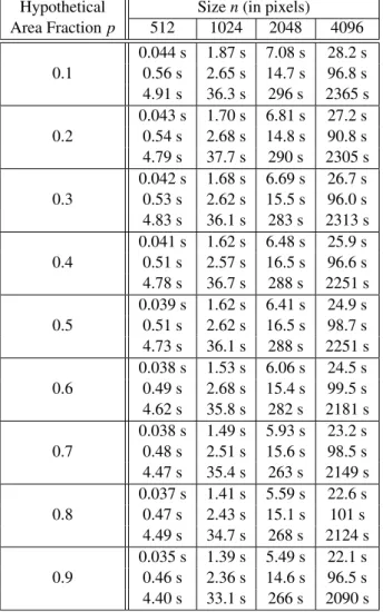
Table 1. Execution times of the novel (above), the

improved (middle), and the direct (below) algorithm (excluding the execution time for the distance transforms).

Hypothetical Sizen(in pixels)

(7)

Table 2. Execution times of the novel (above), the improved (middle), and the direct (below) algorithm (including the execution time for the distance transforms).

Hypothetical Sizen(in pixels) Area Fractionp 512 1024 2048 4096

0.044 s 1.87 s 7.08 s 28.2 s 0.1 0.56 s 2.65 s 14.7 s 96.8 s 4.91 s 36.3 s 296 s 2365 s 0.043 s 1.70 s 6.81 s 27.2 s 0.2 0.54 s 2.68 s 14.8 s 90.8 s 4.79 s 37.7 s 290 s 2305 s 0.042 s 1.68 s 6.69 s 26.7 s 0.3 0.53 s 2.62 s 15.5 s 96.0 s 4.83 s 36.1 s 283 s 2313 s 0.041 s 1.62 s 6.48 s 25.9 s 0.4 0.51 s 2.57 s 16.5 s 96.6 s 4.78 s 36.7 s 288 s 2251 s 0.039 s 1.62 s 6.41 s 24.9 s 0.5 0.51 s 2.62 s 16.5 s 98.7 s 4.73 s 36.1 s 288 s 2251 s 0.038 s 1.53 s 6.06 s 24.5 s 0.6 0.49 s 2.68 s 15.4 s 99.5 s 4.62 s 35.8 s 282 s 2181 s 0.038 s 1.49 s 5.93 s 23.2 s 0.7 0.48 s 2.51 s 15.6 s 98.5 s 4.47 s 35.4 s 263 s 2149 s 0.037 s 1.41 s 5.59 s 22.6 s 0.8 0.47 s 2.43 s 15.1 s 101 s

4.49 s 34.7 s 268 s 2124 s 0.035 s 1.39 s 5.49 s 22.1 s 0.9 0.46 s 2.36 s 14.6 s 96.5 s 4.40 s 33.1 s 266 s 2090 s

Experimental results show that the novel algorithm is also in practice much better than simpler algorithms. The Boolean model has been chosen for the experiments. Since there is no major dependency between the running-time of the algorithms and the image data, this is representative.

The presented algorithms can also be used to compute estimators of contact distribution functions, since distance distribution functions and contact distribution functions are related to each other as shown.

ACKNOWLEDGMENTS

The author is grateful to Volker Schmidt for valuable comments. He also wants to thank Klaus Mecke for helpful remarks which initiated the experimental part of this work.

REFERENCES

Bhattacharya A (2003). Measurement of Contact Distribution Functions on 2d Binary Images Using Image Processing Techniques. Diploma Thesis, University of Kaiserslautern.

Breu H, Gil J, Kirkpatrick D, Werman M (1995). Linear Time Euclidean Distance Algorithms. IEEE Trans Pattern Anal 17:529-33.

Danielsson PE (1980). Euclidean Distance Mapping. Comput Vision Graph 14:227-48.

Lang C, Ohser J, Hilfer R (2001). On the Analysis of Spatial Binary Images. J Microsc 202:1-12.

Mattfeldt T, Schmidt V, Reepschl¨ager D, Rose C, Frey H (1996). Centered Contact Density Functions for the Statistical Analysis of Random Sets. J Microsc 183:158-69.

Mecke K (1998). Integral Geometry and Statistical Physics. Int J Mod Phys B 12:861-99.

Mecke K, Buchert T, Wagner H (1994). Robust Morphological Measures for Large-Scale Structure in the Universe. Astron Astrophys 288:697-704.

Ohser J, M¨ucklich F (2000). Statistical Analysis of Microstructures in Materials Science. Chichester: John Wiley & Sons.

Ohser J, Steinbach B, Lang C (1998). Efficient Texture Analysis of Binary Images. J Microsc 188:20-8. Ragnemalm I (1993). The Euclidean Distance Transform.

Ph.D. Thesis, University of Link¨oping.

Rosenfeld A, Pfaltz J (1966). Sequential Operations in Digital Picture Processing. J ACM 13:471-94.

Rosenfeld A, Pfaltz J (1968). Distance Functions in Digital Pictures, Patt Recogn 1:33-61.

Serra J (1982). Image Analysis and Mathematical Morphology. London: Academic Press.

Soille P (1991). Spatial Distributions from Contour Lines: An Efficient Methodology Based on Distance Transformations. J Vis Commun Image R 2:138-50. Stoyan D, Kendall WS, Mecke J (1995). Stochastic

Geometry and its Applications. Chichester: John Wiley & Sons.

Stoyan D, Stoyan H, Tscheschel A, Mattfeldt T (2001). On the Estimation of Distance Distribution Functions for Point Processes and Random Sets. Image Anal Stereol 20:65-9.