Predictive Query Indexing for Ambiguous Moving Objects in Uncertain
Data Mining
Gowri Sree Lakshmi Neeli1*, Kesavarao Seerapu2
#1. M.Tech (CSE) in Department of Computer Science Engineering,
#2. Assist.Prof, Department of Computer Science and Engineering, Avanthi Institute of Engineering &Technology, Vizianagaram, AP, INDIA.
Abstract
Indexing and query processing is a developing examination field in spatio-temporal data. The majority of the continuous applications, for example, area based administrations, armada administration, movement expectation and radio recurrence recognizable proof and sensor systems depend on spatiotemporal indexing and query preparing. All the indexing and query processing applications is any of the structures, for example, spatio file get to and supporting inquiries or spatio-transient indexing technique and bolster query or temporal measurement, while in spatial data it is considered as the second need. The majority of the current overview takes a shot at spatio-fleeting depend on indexing techniques and query preparing, yet exhibited independently. Probabilistic range query is an essential kind of query in the region of dubious data administration. A probabilistic range query restores every one of the articles inside a particular range from the query question with a likelihood no not as much as a given edge. A query protest is either a specific question or an indeterminate question demonstrated by a Gaussian appropriation. We propose a few sifting systems and a U-tree-based list to effectively bolster probabilistic range questions over Gaussian items. Broad tests on genuine data exhibit the proficiency of our proposed approach. Keywords: Uncertain Data, Constrained space, probabilistic range query, uncertain moving objects, obstacles, query processing.
I. Introduction
As of late, uncertain data administration has gotten significant consideration in the database group. It includes an extensive assortment of true applications, going from versatile mechanical autonomy, sensor systems to area based administrations. Among every one of the issues in the zone of indeterminate data
likelihood [8] for every data question and yield it if this likelihood is no not as much as the limit. In any case, the likelihood calculation for the most part requires exorbitant numerical joining for precise outcome [6], rendering it restrictively costly to process for every one of the data questions and check if the query limitation is fulfilled. In this manner, such calculations ought to be decreased however much as could be expected. There have been answers for probabilistic range questions that can deal with Gaussian-based dubious data, yet in light of particular suppositions. For instance, U-tree [2] accept that each indeterminate question is situated inside a pre-characterized instability area. It builds a list for all articles in view of this area to lessen the quantity of hopefuls that require the costly numerical coordination. In addition, Gauss-tree [3] is proposed for probabilistic recognizable proof inquiries, however the Gaussian dispersions they take after must be autonomous in each measurement. At the point when these suspicions are disregarded, these arrangements at no time in the future work. One issue of U-tree is that it is difficult to choose a reasonable degree of the instability district for a certifiable protest. In this paper we take care of these issues with nonexclusive Gaussian circulations with no of these suppositions; i.e., the items can situate in an endless space rather than U-tree, or have connections between's measurements instead of Gauss-tree. II. Related Work
Query Processing on Imprecise Data Early research fundamentally concentrates on different data models for precisely catching the areas of moving articles. In this specific circumstance, query calculations go for limiting the measure of data transmission (for refreshing the focal server) to guarantee the exactness of database esteems. Cheng et al. [4] are the first to detail questionable recovery all in all areas. They display an intriguing scientific classification of novel query sorts, together with the comparing preparing techniques. An I/O effective calculation for closest neighbor pursuit is proposed in [5]. Nothing from what was just mentioned works considers prob-go recovery. Cheng et al. [6] build up a few answers for prob-extend inquiries which, in any case, target 1D space as it were. They contend that range seek in unverifiable databases is intrinsically more troublesome than that on conventional exact questions, and bolster their cases by giving two hypothetical methodologies that accomplish (practically) asymptotically ideal execution. All
things considered, the practicability of these techniques is restricted since (i) they can't bolster objects with subjective pdfs (e.g., one strategy targets just uniform pdfs), and (ii) they may bring about expansive real execution overhead because of the concealed constants in their unpredictability ensures. Dalvi and Suciu [8] examine "probabilistic databases", where each record is the same as a tuple in a customary database, aside from that it is related with an "existential" likelihood. For instance, a 60% existential likelihood implies that a tuple may not exist in the database with a 40% possibility; in the event that it does, nonetheless, its esteems are exact. Henceforth, probabilistic databases are not the same as indeterminate databases (the theme of this paper), where each protest unquestionably exists however its solid esteems take after a probabilistic dispersion. A productive stream mining calculations was planned in [17] to mine regular examples successfully and effectively from such spilling data.In [18], a tree-based mining calculation was created that used to mine continuous examples from dynamic indeterminate data stream in light of time-blurring and historic point models.An proficient Skyline query calculation was composed in [19] of questionable moving stream data yet the execution is neglected to utilize list structures, for example, lattice, R tree et cetera. A novel calculation was viably composed in [20] to mine the questionable gathering designs that enhance the mining productivity however it not proficient to deal with more unpredictable examples. The previously mentioned challenges related with various data mining procedures hard to handle the data instability issue viably. Henceforth, a novel approach called Fusion Layer Topological Space Query (FLTS) Indexing system is acquainted with take care of the questionable data mining issue on preparing the client asked for query. The concise clarification about the FLTS Indexing procedure is introduced in next segment.
III. Data Uncertainty and Probabilistic Queries
In [7][9], a data representation scheme known as
probabilistic uncertainty model was proposed. The
model requires that at the time of query execution, the range of possible values of the attribute of interest, and their distributions, are known. For notational convenience, we assume that a real-valued attribute a of a set of database objects T is queried. The ith object of T is named Ti, and the value of a for
continuous random variable. The probabilistic
uncertainty of Ti.a consists of two components:
Definition 1 An uncertainty interval of Ti.a, denoted
by Ui, is an interval [Li,Ri] where Li,Ri∈ <, and the
conditions Ri≥Liand Ti.a∈Uialways hold.
Definition 2 An uncertainty pdf of Ti.a, denoted by
fi(x), is a pdf of Ti.a, such that fi(x)=0 if x∈/ Ui.
This simple model provides flexibility where the exact model of uncertainty is determined by applicationdependent assumptions. A simple example is the modeling of sensor measurement uncertainty, where each Uiis an error range containing the mean
value, and fi(x) is a normal distribution. Another
example is the modeling of one-dimensional moving objects based on [20], where at any point in time, the actual location is within a certain bound, d, of its last reported location value. If the actual location changes further than d, then the sensor reports its new location value to the database and possibly changes d. In this case, Uicontains all the values within a distance of d
from its last reported value. For fi(x), one may assume
that Ti.a is uniformly distributed, i.e., fi(x) = 1/[Ri−
Li] for Ti.a ∈ Ui. Treating fi(x) as a uniform pdf
models the scenario where Ti.a has an equal chance
of locating anywhere in Ui. Due to its simplicity, a
uniform distribution facilitates ease of analysis and efficient index design, as illustrated in subsequent sections.
Alternatively, one may perform an estimation of the pdf based on time-series analysis, the discussion of which is beyond the scope of this paper. Interested readers are referred to [5] for details. Also notice that we limit our discussion of uncertainty to interval data. A comprehensive discussion of different types of uncertainty can be found in [21].
A probabilistic threshold query (PTQ), proposed in [9], is a variant of probabilistic query, where only answers with probability values over a certain threshold p are returned. The PTQ that we study specifically in this paper is defined formally below. Definition 3 Probabilistic Threshold Query (PTQ)
Given a closed interval [a,b], where a,b∈< and a≤
b, a PTQ returns a set of tuples Ti, such that the
probability Ti.a is inside [a,b], denoted by pi, is
greater than or equal to p, where 0 < p≤ 1.
Simply speaking, a PTQ can be treated as a range query, operating on probabilistic uncertainty
information, and returns items whose probabilities of satisfying the query exceed p.
A Simple Uncertainty Index
A naive method to evaluate a PTQ is to first retrieve all Ti’s, whose uncertainty intervals have some
overlapping with [a,b], into a set S. Each Tiin S is
then evaluated for their probability of satisfying the PTQ with the following operation:
(1)
where piis the probability that Tisatisfies the PTQ,
and OI is the interval of overlap between [a,b] and
Ui.
The answer only includes Ti’s whose pi’s are larger
than p.
Two problems can be seen from this approach. First, how can we find the elements of S i.e., Ui’s that
overlap with [a,b]? It can be very inefficient if each item Tiis retrieved from a large database and tested
against [a,b]. A typical solution is to build an index structure over Ui’s (which are intervals) and apply a
range search of [a,b] over the index. This problem is known as the interval indexing problem, and has been well studied [17][15].
The second problem is that the probability of each element in S needs to be evaluated with Equation 1. This can be a computationally expensive operation. Notice that the bottleneck incurred in this step is independent of whether we use an interval index or not. In particular, the interval index does not help much if many items overlap with [a,b], but most have probability less than p. In this situation, we still need to spend a lot of time to compute the probability values for a vast number of items, only to find that they do not satisfy the PTQ after all.
Probability Threshold Indexing
only a small fraction of them contribute to the results of PTQ.
Our goal is to redesign index structures so that probabilistic uncertainty information is fully utilized during an index search. This structure, called
Probability Threshold Indexing (PTI), is based on the
modification of a one-dimensional U-tree, where probability information is augmented to its internal nodes to facilitate pruning. To illustrate our idea, let us review briefly how a range query is performed on an U-tree. Starting from the root node, the query interval [a,b] is compared with the maximum bounding rectangle (MBR) of each child in the node. Only children with MBRs that overlap with [a,b] are further followed. We thus save the effort of retrieving nodes whose MBRs do not overlap [a,b]. We can generalize this idea by constructing tighter bounds (that we call x-bounds) than the MBR in each node, by using uncertainty information of intervals, so as to further reduce the chance of examining the children of the node. Let Mj denote the MBR/uncertainty
interval represented by the jth node of an U-tree, ordered by a pre-order traversal. Then the x-bound of
Mjis defined as follows.
Definition An x-bound of an MBR/uncertainty
interval Mjis a pair of lines, namely left-x-bound
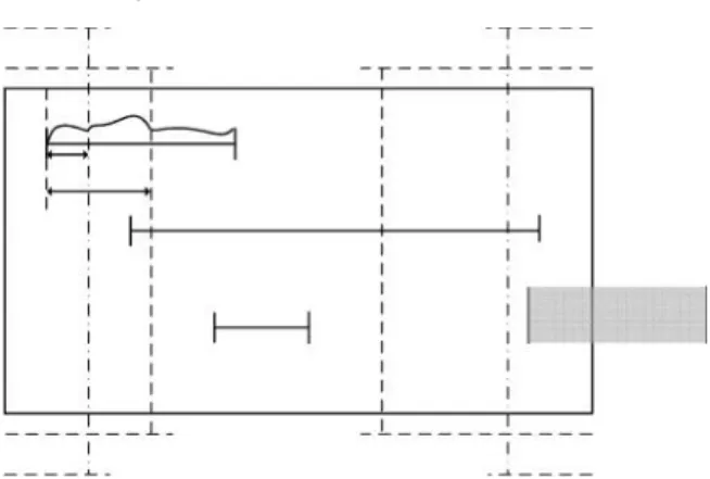
Figure 1: Inside an MBR Mj, with a 0.2-bound and
0.3-bound. A PTQ named Q is shown as an interval.
(denoted by Mj.lb(x)) and right-x-bound (denoted by
Mj.rb(x)). Every interval [Li,Ri] contained in this
MBR is guaranteed to have a probability of at most x
(where 0≤ x≤ 1) of being left of the left-xbound and
being right of the right-x-bound. That is to say, if Li≤
Mj.lb(x) and Ri≥ Mj.rb(x), then the following must
hold: and
.
Using the definition of an x-bound, the MBR of an internal node can be viewed as a 0-bound, since it guarantees all intervals in the node are contained in it with probability one i.e., no interval lies beyond the 0-bound. Figure 1 illustrates three children MBRs (A,B,C), in the form of one-dimensional intervals, contained in larger MBR Mj. A 0.2-bound and a
0.3bound for Mjare also shown.
As Figure 1 shows, an x-bound is a pair of lines where at most a fraction of x of each interval in the MBR cross either of them. For illustration, the uncertainty pdf of A is shown, where we can see that
M .lb(0.2) M b fi(x)dx≤
0.2, and 0.3. For interval B, the constraint on the
right-0.3bound is Interval
C does not crosses either the 0.2-bound and the
0.3-bound, so it satisfies the constraints of both x-bounds. Furthermore, we require an x-bound to be unique, where the left-x-bound and right-x-bound are pushed towards the center of the MBR as much as possible, without violating their definitions.
The whole purpose of storing the information of the
x-bound in a U-tree node is to avoid investigating the
contents of a node. If we can avoid this probing, a considerable amount of I/Os can be saved. Furthermore, we do not need to compute the probability values of those intervals, which cannot satisfy the query anyway. To illustrate how this idea works, let us look at Figure 1 again. Here a range query Q, represented as an interval, is tested against the internal node. Without the aid of the x-bound, Q has to (i) examine which MBR (i.e., A, B, or C) overlaps with Q’s interval, (ii) for the qualified
MBRs (B in this example), further retrieve the node pointed by B until the leaf level is reached, and (iii) compute the probability of the interval in the leaf level.
The presence of the x-bound allows us to decide with ease whether an internal node contains any qualifying MBRs, without further probing into the subtrees of this node. In this example, we first test Q’s range
against the left-0.2-bound and the right-0.2bound. As shown in Figure 1, it intersects none of these bounds. In particular, although Q overlaps the MBR, its overlapping region is somewhere between the right-0.2-bound and the right boundary of Mj’s MBR.
This implies that the portion of the intervals (interval
B) that passes through the 0.2-bound cannot exceed a
probability of 0.2. Therefore, the probability of intervals in the MBR that overlap the range of Q cannot be larger than 0.2. Assume Q has a probability threshold of 0.3 i.e., Q only accepts intervals with an overlapping probability of at least 0.3. Then we can be certain that none of the intervals in the MBR satisfies Q, without further probing the subtrees of this node. Compared with the case where no x-bounds are implanted, this represents a significant saving in terms of number of I/Os and computation time.
In general, given an x-bound of a MBR Mj, we can
eliminate Mj from further examination if the
following two conditions hold:
1. [a,b] does not intersect left-x-bound or
right-xbound of Mj i.e., either b < Mj.lb(x) or a >
Mj.rb(x) is true, and
2. p≥x
If no x-bound in Mjsatisfies these two conditions, the
checking of intersections with Mjis resumed, where
the contents of the node represented by Mjare loaded,
and the range searching process is done in the same manner for an U-tree.
IV. A Simple Uncertainty Index
Answer Range Queries over Imprecise Data
In this section, we show how to answer the two range queries described earlier. Although the process is straightforward, the format of results is important for further discussions in the later sections. Here different objects may have different imprecision e. Note although we assume a uniform probability distribution of object location across the uncertain area, any type of known probability distribution is applicable.
Return Objects in a Given Range
The task of returning objects within a given query range can be accomplished by modifying the traditional spatial query processing technique that deploys tree structures. The first modification is that the point objects are now represented by objects with non-zero extents—the uncertain area with radius
e(see figure 1). To handle the fact that some objects
are not fully contained in the region, another modification is needed to associate each returned
object with a probability value(pi) to indicate how
likely the object can really be in the query region.
Fig.2 Range Query over Imprecise Fig.3 Effect of Imprecision e in Range
Data (sets differentiated by colors) Query
Probability value piis 1.0 for those objects whose
uncertainty area is completely contained by the given query region. For objects whose uncertainty areas overlap with query region, picould be computed as
the cumulative probability represented by the overlapping area. Under the assumption of uniform probability distribution, we have: , where Ai
is the overlap area that can be computed from geometric parameters.
Return COUNT of Objects in a Given Range
To answer COUNT queries, the format of answers needs to be specified first. Possible options are {min,max}, {min,max,mean}, {min,max,mean,var}, and {(min,Pmin),(min + 1,Pmin+1),...,(max,Pmax)}. Note
that here we use upper case P to represent the probability that COUNT takes a specific value. Lower case p is used to represent the probability with which an object could be in a query region. A server can produce all the information needed in the above answer formats, given its capability to answer the query discussed in section 3.1. Here we summarize the process to compute the above answers.
Let the first Nsobjects in the answer set be the ones
from MUST set. Then, we know pi= 1 for all 1≤i≤
Ns. An immediate result is that min = |MUST| = Ns
and max = |MUST|+|MAY | = Ns +Nm. Mean is
summation of pi’s of all relevant objects. And
variance can be evaluated as:
Ns+Nm
k=0
The probability for individual COUNT value can be computed by summation of probabilities of events that yield the COUNT. For example, below is the probability that COUNT takes value of min + 1.
Ns+Nm
P(COUNT = Ns+ 1) = X pi[Y(1−pj)] (2)
i,j=Ns+1 j6=i
Among the four answer formats, the more detailed formats require more computation as well as larger answer sizes. Choosing a proper format should be a task of database server based on user requirements. In next section, we base our discussion on the second format.
R-tree Based CPA Join
Given these caveats, perhaps the most natural choice for the CPA Join is the R-tree. The R-tree is a hierarchical, multi-dimensional index structure that is commonly used to index spatial objects. The join problem has been studied extensively for R-trees and several spatial join techniques exist that leverage underlying R-tree index structures to speed-up join processing. Hence, our fi inclination is to consider a spatiotemporal join strategy that is based on R-trees. The basic idea is to index object histories using R-trees and then perform a join over these indices. The R-Tree Index
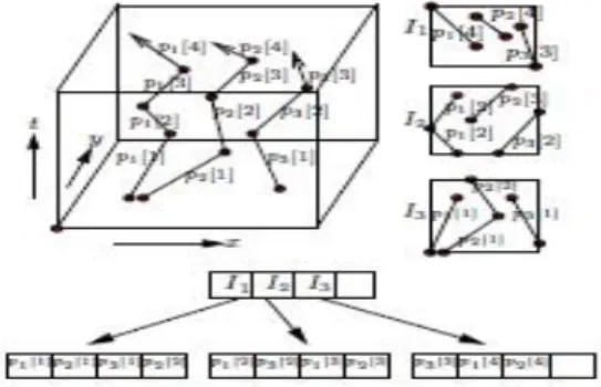
It is a very straightforward task to adapt the R-tree to index a history of moving object trajectories. Assuming three spatial dimensions and a fourth temporal dimension, the four-dimensional line segments making up each individual object trajectory are simply treated as individual spatial objects and indexed directly by the R-tree. The R-tree and its associated insertion or packing algorithms are used to group those line segments into disk-page sized groups, based on proximity in their four-dimensional space. These pages make up the leaf level of the tree. As in a standard R-tree, these leaf pages are indexed by computing the minimum bounding rectangle that encloses the set of objects stored in each leaf page. Those rectangles are in turn grouped into disk-page sized groups which are themselves indexed. An R-tree index for 3 line segments moving through 2-dimensional space is depicted in Figure 4.
Figure 4. Example of an R-tree
Basic CPA Join Algorithm Using R-Trees
Assuming that the two spatiotemporal relations to be joined are organized using R-trees, we can use one of the standard R-tree distance joins as a basis for the CPA Join. The common approach to joins using R-trees employ carefully controlled synchronized traversal of the two R-trees to be joined. The pruning power of the R-tree index arises from the fact that if two bounding rectangles R1 and R2 do not satisfy the join predicate then the join predicate is not satisfied between any two bounding rectangles that can be enclosed within R1 or R2.
Figure 5. Heuristic to speed up distance computation V. Proposed Methodology
The distance routine is used in evaluating the join predicate to determine the distance between two bounding rectangles associated with a pair of nodes. A node-pair qualifies for further expansion if the distance between the pair is less than the limiting distance d supplied by the query. Objects moving in a constrained 2D space where objects are forbidden to be located in some specific areas such specific areas as restricted areas, and dub the query above the Constrained Space Probabilistic Range Query (CSPRQ). The CSPRQ can also find many applications as objects moving in a constrained 2D space are common in the real world. For example, the tanks in the digital battlefield usually cannot run in lakes, forests and the like, the areas occupied by those obstacles can be naturally regarded as restricted areas. The key idea of proposed solution is to use a strategy called pre-approximation that can reduce the initial problem to a highly simplified version, implying that it makes the rest of steps easy to tackle. The optimizations are mainly based on two insights: (i) the number of effective subdivisions is no more than 1, we utilize this insight to improve the power pruning restricted areas; and (ii) an entity with the larger span is more likely to subdivide a single region, this insight motivates us to sort the entities to be processed according to their spans. In addition to the main insights above, we also realize two other facts and utilize them. Specifically, two mechanisms are developed: postpone processing and lazy update. VI. Performance Evaluation
The average query response time of 200 PRQ-P (resp. PRQ-G) queries (10K samples are used for numerical integration) is 0.242 seconds (1.250 seconds resp. PRQ-G) for G-tree, and 120.764 seconds (236.725 seconds resp. PRQ-G) for Scan, almost 500 (190 resp. PRQ-G) times that of G-tree. Among the overall response time, the integral computation takes up 0.237 seconds (1.246 seconds resp. PRQ-G) for G-tree, and 120.692 seconds (236.577 seconds resp. PRQ-G) for Scan. This indicates that probability integration dominates the overall query processing and is computationally expensive. Consequently, it is important to reduce candidate objects which need to perform integration as much as possible.
Among 50,747 objects in LB, the average candidate number of G-tree is 93 for PRQ-P (335 for PRQ-G). The number of validated objects by integration is 65 for PRQ-P (156 for PRQ-G). So for PRQ-P 69.9% (46.6% for PRQ-G) of the candidates identified by our approach are real results. This demonstrates the effectiveness of our proposed filtering techniques. In the sequel, we exclude the integral part from query processing and focus on evaluating the filtering and indexing performance of FR-tree and G-tree.
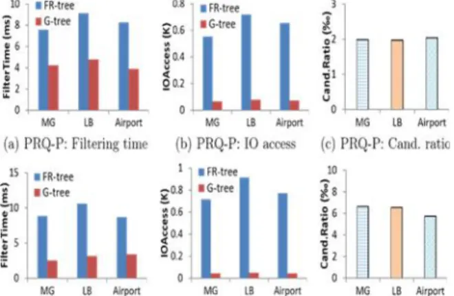
We run the two algorithms to process 10K queries on the three datasets and show the average filtering time and IO access of PRQ-P (resp. PRQ-G) in Fig. 6(a)–
6(b) (resp. Fig. 6(d)– 6(e)). For PRQ-P, the filtering time of G-tree is half of that of FR-tree, because the IO access of G-tree is 90% less than that of FR-tree, though the segmented bounding boxes in G-tree are more complex to process than those in FR-tree. The reduction on PRQ-G is more substantial. The filtering time of G-tree on MG and LB is 71% less than that of FR-tree, and 61% on Airport. The IO access of G-tree of three datasets is 6% that of FR-tree.
As aρmaxis adopted to process queries with anyθ, the bounding boxes in FR-tree are very loose. This causes more IO accesses and increases filtering time. On the other hand, since the bounding boxes in G-tree are constructed in a parametric fashion, they can be calculated dynamically for arbitrary θ and hence are compact. Another interesting observation is that the IO access almost resembles the candidate number, indicating most IOs are spent on retrieving data objects.
same since we equip FR-tree with our filtering techniques.
(d) PRQ-G: Filtering time (e) PRQ-G: IO access (f) PRQ-G: Cand. ratio
Fig.6. Performance of PRQ-P and PRQ-G Queries
The candidate ratio is around 2‰ for PRQ-P and 6‰
for PRQ-G on the three datasets. This reveals that only a very small percentage of data objects will become candidates owing to our filtering techniques. Varying Dataset Size. To evaluate the scalability of our approach, we randomly extract 20%, 40%, 60%, 80% and 100% of LB dataset and show the filtering time and IO access of two methods in Fig. 7(a)–7(b) on PRQ-P queries. The performance on PRQ-G queries reveals a similar trend and hence is omitted here due to space limit. As the dataset size becomes larger, the filtering time and IO access of FR-tree almost increase linearly. G-tree displays a steady increasing trend and always outperforms FT-tree.
(a) PRQ-P: Filtering time (b) PRQ-P: IO access Fig. 7 Varying [D]: Filtering time and IO access (PRQ-P)
(a) PRQ-P: Candidate ratio (b) PRQ-G: Candidate ratio
Fig.8. Varying |D|: Candidate ratio
As shown in Fig. 8(a) – 8(b), the candidate ratio of PRQ-P retains 2‰ when varying the dataset size |D|, and 6.5‰ for PRQ-G, demonstrating the steadiness and scalability of our approach with respect to the dataset size.
Varying Query Range. We vary the query range δ from 10 to 100 by 10 and show the performance on
PRQ-P queries in Fig. 9(a)– 9(b). The performance on PRQ-G queries is similar and hence omitted. Asδ increases, FR-tree consumes much more time and more IO accesses on filtering processing. In contrast, Gtree exhibits much slower increasing trends. Fig. 10(a)– 10(b) shows that the candidate ratio of both PRQ-P and PRQ-G also increases with δ, but for PRQ-P it is only 3.4% (11.6% for PRQ-G) even if achieves 100.
(a) PRQ-P: Filtering time (b) PRQ-P: IO access Fig. 9. Varying: Filtering time and IO access (PRQ-P)
(a) PRQ-P: Candidate ratio (b) PRQ-G: Candidate ratio
Fig.10. Varyingδ: Candidate ratio
Varying Probability Threshold. We varyθfrom 0.1 to 0.9 and show the performance in Fig. 11(a)–12(b) for both PRQ-P and PRQ-G queries. For PRQ-P, the filtering time and IO access of both FR-tree and G-tree decreases gradually with θ when it is less than 0.5. When θ exceeds 0.5, the filtering time slightly rebounds. This is consistent with our filtering condition which assignsρ= 1− 2θifθ <0.5 andρ= θifθ≥ 0.5. Because whenθ <0.5,ρdecreases when θ moves towards larger values, and bounding boxes shrink. So most of non-candidates can be filtered quickly and and less IO accesses are needed, and hence it accelerates filtering.
in filtering time is not obvious in this case. The reason also accounts for the trend of G-tree on candidate ratio in Fig. 10
VII. Conclusion
The CSPRQ for uncertain moving objects. The deliberate analyses offer insights into the problem considered, and show that to process the CSPRQ using a straightforward method is infeasible. We propose the targeted solution and demonstrate its efficiency and effectiveness through extensive experiments. An additional finding is the precomputation based method has a non-trivial preprocessing time (although it outperforms our preferred solution in other aspects), which offers an important indication sign for the future research. We conclude this paper with several interesting research topics: (i) how to process the CSPRQ in 3D space (ii) if the location update policy is the time based update, rendering that the uncertainty region u is to be a continuously changing geometry over time, how to process the CSPRQ in such a scenario (iii) if the query issuer is also moving, the location of query issuer is also uncertain, how to process the location based CSPRQ.
REFERENCES
[1] M. D. Berg, O. Cheong, M. V. Kreveld, and M. Overmars, Computational Geometry: Algorithms and Applications, 3rd Ed. Berlin, Germany: Springer, 2008.
[2] B. Braden, “The surveyor’s area formula,”
College Math. J., vol. 17, no. 4, pp. 326–337, 1986.
[3] J. Chen and R. Cheng, “Efficient evaluation of imprecise location dependent queries,” in Proc. IEEE
Int. Conf. Data Eng., 2007, pp. 586–595.
[4] R. Cheng, D. V. Kalashnikov, and S. Prabhakar,
“Querying imprecise data in moving object environments,” IEEE Trans. Knowl. Data Eng., vol.
16, no. 9, pp. 1112–1127, 2004.
[5] B.S. E. Chung, W.-C. Lee, and A. L. P. Chen,
“Processing probabilistic spatio-temporal range
queries over moving objects with uncertainty,” in
Proc. Int. Conf. Extending Database Technol., 2009, pp. 60–71.
[6] T. Emrich, H.-P. Kriegel, N. Mamoulis, M. Renz, and A. Z€ufle, “Querying uncertain spatio-temporal
data,” in Proc. IEEE Int. Conf. Data Eng., 2012, pp.
354–365.
[7] B. Gedik, K.-L. Wu, P. S. Yu, and L. Liu,
“Processing moving queries over moving objects
using motion-adaptive indexes,” IEEE Trans.Knowl. Data Eng., vol. 18, no. 5, pp. 651–668, 2006.
[8] G. Greiner and K. Hormannn, “Efficient clipping of arbitrary polygons,” ACM Trans. Graph., vol. 17,
no. 2, pp. 71–83, 1998.
[9] K. Hormann and A. Agathos, “The point in
polygon problem for arbitrary polygons,” Comput.
Geometry, vol. 20, no. 3, pp. 131–144, 2001.
[10] H. Hu, J. Xu, and D. L. Lee, “A generic
framework for monitoring continuous spatial queries
over moving objects,” ACM Int. Conf. Manag. Data,
2005, pp. 479–490. Authors
Gowri SreeLakshmi Neeli currently pursing Post Graduation (M.TECH) in
AVANTHI ENGINEERING
COLLEGE affiliated to Jawaharlal Nehru Technological University, Kakinada from 2015-2017 in the department of computer science Engineering. She completed post-Graduation (MSC(cs)) in the year 2008 from Gitam college, Vishakapatnam which is affiliated under Andhra University.