On Some Aspects of a Generalized Asymmetric Normal Distribution

ON SOME ASPECTS OF A GENERALIZED ASYMMETRIC

NORMAL DISTRIBUTION

C. Satheesh Kumar1

Department of Statistics, University of Kerala, Trivandrum, India G.V. Anila

Department of Statistics, University of Kerala, Trivandrum, India

1. INTRODUCTION

The normal distribution is the basis of many statistical works and it enjoys a unique po-sition in probability theory. It is an unavoidable tool for the analysis and interpretation of data. In many practical applications it has been observed that real life data sets are not symmetric. They exhibit some skewness, therefore do not conform to the normal distribution, which is popular and easy to be handled. Azzalini (1985) introduced a new class of distributions namely “the skew normal distribution”, which is mathematically tractable and includes the normal distribution as a special case. This family of distri-butions is well known for modeling and analyzing skewed data. This distribution has been developed via standard normal probability density function (p.d.f) and cumulative distribution function (c.d.f) through adding a shape parameter to regulate skewness, so as to have more flexibility in fitting real life data sets.

Let f(.)andF(.)be the p.d.f and c.d.f of a standard normal variate. Then a ran-dom variableX is said to follow the skew normal distribution with parameterλ∈R= (−∞,∞)if its probability density function (p.d.f.) h(x;λ)is of the following form. Forx∈R,

h(x;λ) =2f (x)F(λx), (1) hereafter, we denoted a distribution with p.d.f. (1) asSN D(λ). This distribution has been studied by several authors such as Azzalini (1986), Henze (1986), Liseo (1990), Azzalini and Dalla Valle (1996), Branco and Dey (2001), Gentonet al.(2001), Loperfido (2001), Gupta and Kollo (2003), Loperfido (2004), Genton (2004), Genton and Loperfido (2005), Lachoset al.(2007), Guptaet al.(2007), Kim (2008), Wanget al.(2009) and Kumar and Anusree (2011, 2013, 2014a,b).

The normal and skew normal models are not adequate to describe the situations of plurimodality. To overcome this drawback Kumar and Anusree (2011) considered a new class of generalized skew normal distribution as a generalized mixture of standard normal and skew normal distributions through the following p.d.f in which x ∈ R,

λ∈Randα >−1.

h₁(x;λ,α) = 2

α+2f (x)[1+αF(λx)]. (2)

The distribution given in (2) they termed as generalized mixture of standard normal and skew normal distributions(GM N SN(α,λ)). ClearlyGM N SN(−1,λ)isSN(−λ). In order to develop a more flexible plurimodal asymmetric normal distribution, through the present paper we consider a generalized version of the skew normal distribution of Kumar and Anusree (2011) which we call “the generalized asymmetric normal distribu-tion (GAND)”.

The organization of the paper is as follows. In Section 2 we present the definition and some properties of the GAND. In Section 3 certain reliability measures such as re-liability function, failure rate, and mean residual life function are derived and condition for unimodal and plurimodal situations are obtained. In Section 4 a location scale exten-sion of the GAND is proposed and derive its important properties such as characteristic function, mean, variance, measure of skewness and kurtosis, reliability measures etc. Further in Section 5 we discuss the maximum likelihood estimation of the parameters of extended GAND and a real life application of the distribution is considered in Section 6.

2. THE GENERALIZED ASYMMETRIC NORMAL DISTRIBUTION

Here we define a new class of generalized skew normal distribution and derive some of its important properties.

DEFINITION1. A random variable X is said to have a generalized asymmetric normal distribution if its p.d.f is of the following form, in which x∈R,λ,β,∈R andα >−1.

g(x;α,λ,β) = f(x)

α+2

h

2+α[F(β)]−1F(λx+βp1+λ2₎i_{. (3)} Here f(.) and F(.) are p.d.f and c.d.f of standard normal variate. A distribution with p.d.f (3) we denoted as GAND(α,λ,β). Note that whenβ=0GAND(α,λ,β) reduces to skew normal distribution of Kumar and Anusree (2011).

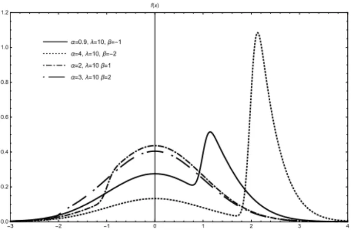
For some particular choices ofα,λandβthe p.d.f. given in (3) of GAND(α,λ,β) is plotted in Figures 1 and 2.

α0.9,λ10,β=-1

α=4,λ=10,β=-2

α=2,λ=10β=1

α=3,λ=10β=2

-3 -2 -1 0 1 2 3 4 0.0

0.2 0.4 0.6 0.8 1.0 1.2

f(x)

Figure 1 –Probability plots of GAND(α,λ,β) for fixed values ofλand various values ofαandβ.

α2,λ5,β=-1

α=3,λ=5,β=-2

α=0.5,λ=5β=-3

α=1,λ=5β=-5

-3 -2 -1 0 1 2 3 4

0.0 0.2 0.4 0.6 0.8

f

PROOF. The p.d.fg₁(y₁)ofY₁is

g₁(y₁) = g(−y₁;α,λ,β)|d x d y₁|

= f(−y1)

α+2

h

2+α[F(β)]−1_F(−λy 1+β

p

1+λ2₎i

= g(y₁;α,−λ,β),

since f(.)is the p.d.f. of standard normal variate. HenceY₁follows GAND(α,−λ,β).

2

RESULT2. If X has GAND(α,λ,β) then Y₂ = X2 has a p.d.f (4) in which∆(y) = F(λy+βp1+λ2_{) +F(−λy+β}p_1+λ2_).

PROOF. The p.d.f. g₂(y₂)ofY₂=X2is the following, fory₂>0.

g₂(y₂) = g(py₂,α,λ,β)|d x d y₂|+g(−

p_y

2,α,λ,β)| d x d y₂|

= f(

p_y 2)

α+2

h

2+α[F(β)]−1F(λpy₂+βp1+λ2₎i 1 2py₂+ f(−py₂)

α+2

h

2+α[F(β)]−1F(−λpy₂+βp1+λ2)i 1 2py₂ = f(

p_y 2) 2(α+2)py₂

h

4+α[F(β)]−1nF(λpy₂+βp1+λ2₎

+F(−λpy₂+βp1+λ2)oi

=

_f(p_y

2) 2py₂

1

(α+2)

4+α[F(β)]−1∆(py₂)

. (4)

2

PROOF. Forx>0, the p.d.f ofg₃(x)ofY₃is g₃(y₃) = g(y₃;α,λ,β)|d x

d y₃|+g(−y3;α,λ,β)| d x d y₃|

= f(y3)

α+2

h

2+α[F(β)]−1_F(λy 3+β

p

1+λ2₎i₊ f(−y₃)

α+2

h

2+α[F(β)]−1F(−λy₃+βp1+λ2₎i

= f(y3)

α+2

h

4+α[F(β)]−1nF(λy₃+βp1+λ2_{) +F(−λy} 3+β

p

1+λ2₎oi

= f(y3)

α+2

4+α[F(β)]−1∆(y₃)

. (5)

2

RESULT4. The cumulative distribution function (c.d.f) G(x)of GAND(α,λ,β) with p.d.f (3) is the following, for x∈R

G(x) = F(x) α+2

h

2+α 2[F(β)]

−1i₋α[F(β)]−1

α+2 ξβ(x,λ), (6)

whereξ_β(x,λ) =R∞

x

Rλx+βp(1+λ2)

0 f (t)f (u)d ud t , which can be evaluated using the soft-ware MATHCAD.

PROOF. G(x) =

Zx

−∞

g(t;α,λ,β)d t

= 2

α+2F(x) +

α[F(β)]−1

α+2





F(x) 2 −

Z∞

x

Zλx+βp1+λ2

0

f(t)f(u)d ud t





= F(x) α+2

h

2+α 2[F(β)]

−1i₋α[F(β)]−1

α+2 ξβ(x,λ).

2

Now we derive the characteristic function of GAND(α,λ,β) and we need the fol-lowing lemma.

LEMMA2. Ellison (1964). For a standard normal random variable X with distribution function F we have the following for all a,b∈R

E{F(aX+b)}=F

b p

1+a2

RESULT5. The characteristic functionφ_X(t)of GAND(α,λ,β) with p.d.f (3) is the following, for t∈R and i=p−1

φX(t) = e−2t2

α+2

2+α[F(β)]−1F(δi t+β)

, (7)

whereδ=pλ

1+λ2.

PROOF. LetX follows GAND(α,λ,β) with p.d.f (3). Then by the definition of characteristic function, we have the following for anyt∈Randi=p−1

φX(t) = E(ei t X)

= 2

α+2

Z∞

−∞

ei t xf(x)d x+α[F(β)]

−1

α+2

Z∞

−∞

ei t xf(x)F(λx+βp1+λ2)_{d x}

= 1

α+2e

−t2 2

2+α[F(β)]−1Z∞

−∞

1 p

2πe

−(x−i t)2

2 F(λx+β

p

1+λ2_{)d x}

. (8) On substitutingx−i t=u, in (8) we obtain

φX(t) = e−2t2

α+2

2+α[F(β)]−1F(δi t+β)

,

which implies (7) in the light of Lemma 2. 2

RESULT6. The nth raw momentµ0_nof GAN D(α,λ,β)with p.d.f (3) is the following, for n≥0

µ0

n= 1

α+2ξr+

α[F(β)]−1

α+2 n

X

r=0

 _n

r

‹

ξ_rϕ_n−r, (9)

where for r =0, 1, 2, ...,n

ξr=







0, if r is odd (−1)r2r!

(r 2)!2

r

2 , if r is even

ϕr=



 

 

(δi)r₍₋₁₎r−₂1_(r−1)!βr−1_f(β)

(r−1 2 )!2

r−1

2 , if r is odd

(δi)r₍₋₁₎r2(r−1)!βr−1_f(β)

PROOF. The characteristic function ofGAN D(α,λ,β)can be written as

φ_X(t) = 2

α+2I(t) +

α[F(β)]−1

α+2 I(t)J(t), (10)

in whichI(t) =e−t22 andJ(t) =F(δi t+β)on differentiating (10) with respect tot,n

times and puttingt=0 we get thent hmoment ofX as

µ0

n=

–

2

α+2I

r_{(t) +}α[F(β)]−1

α+2 n

X

r=0

Ir(t)Jn−r(t)

™

t=0

, (11)

in whichIr(t)andJn−r(t)respectively denote ther t hand(n−r)t hderivative ofI(t) andJ(t)which are obtained as

I(r)(t) = [r

2]

X

j=0

(−1)r−j_tr−2j_r!e−t22

j!2j_(r−2j)! (12)

and

J(r)(t) = [r−1

2 ]

X

k=0

(δi t+β)r−2k−1₍₋₁₎r−k−1_{(r−1)!f(δi t+β)(δi)}r

k!(r−2k−1)!2k . (13)

If we put t = 0 in (12) and (13) and using the notationξr = I(r)(0)andϕn−r =

J(n−r)(0)we get (9) from (11). 2

Using Result 6 we prove the following.

RESULT7. The mean and variance of GAND(α,λ,β) with p.d.f (3) is given by

Mean= α

α+2.

δf(β) F(β) , Variance=−αδβf(β)

(α+2)F(β)+1−

α2_δ2_[f(β)]2

(α+2)2_[F(β)]2.

RESULT8. The measure of skewness(γ₁) and measure of kurtosis (γ₂) of GAND(α,λ,β) with p.d.f (3) are respectively given by

γ1=

(−δ2_d+δ2_dβ2_+3βd2_δ+2d3₎2

(−βd+1−d2)3 and

3. RELIABILITY MEASURES AND MODE

Here we investigate some properties of GAND(α,λ,β) with p.d.f. (3) useful in reliabil-ity studies.

LetX follows GAND(α,λ,β) with p.d.f (3). Now from the definition of reliability functionR(t), failure rater(t)and mean residual life functionµ(t)ofX we obtain the following results.

RESULT9. The reliability function R(t)of X is the following, in whichξ_β(x,λ) =

R∞

x

Rλx+βp(1+λ2)

0 f (t)f (u)d ud t is as defined in Result 4

R(t) = 1

α+2[1−F(t)]

2+α[F(β)]

−1

2

+α[F(β)]−1

α+2 ξβ(t,λ). RESULT10. The failure rate r(t)of X is given by

r(t) = f(t)

”

2+α[F(β)]−1_F(λt+βp_1+λ2₎—

(1−F(t))”2+α[F(₂β)]−1—+α[F(β)]−1_ξ β(t,λ)

.

RESULT11. The mean residual life function of GAND(α,λ,β) is

µ(t) = 1

(α+2)R(t)







1 p

2π



2e

−t2

2 +αλ[F(β)]

−1_e−β₂2 p

1+λ2





+α[F(β)]−1F(λt+βp1+λ2)_f(_t) − αλ[F(β)]−

1 p

2πp1+λ2e

−β2 2 F

p

1+λ2_(t+pλβ 1+λ2)

−t.

(14) PROOF. By definition, the mean residual life function (MRLF) ofX is given by

µ(t) = E(X−t/X >t) = E(X/X >t)−t, where

E(X/X >t) = 1 (α+2)R(t)

Z∞

t

x f(x)d x+ α[F(β)]

−1

(α+2)R(t)

Z∞

t

x f(x)F(λx+βp1+λ2_{)d x}

= 1

(α+2)R(t)[I1+α[F(β)]

−1_I

where

I₁ =

Z∞

t

x f(x)d x

= e

−t2 2

p

2π (16)

I₂ =

Z∞

t

x f(x)F(λx+βp1+λ2_{)d x}

= −

Z∞

t

f0(x)F(λx+βp1+λ2_{)d x}

= F(λt+βp1+λ2_{)f(t) +λ}

Z∞

t

f(λx+βp1+λ2_{)f(x)d x}

= Fλt+βp1+λ2_{f(t) +p} λ 2πp1+λ2e

−β2 2

1−F

p

1+λ2

t+pλβ 1+λ2

. (17)

Now by applying (16) and (17) in (15), we get (14). The functionsR(t),r(t), and

µ(t)are equivalent in the sense that if one of them is given the other two can be uniquely

determined. 2

REMARK3. GAN D(α,λ,β)has increasing failure rate for allαandλand hence de-creasing mean residual life.

RESULT12. Case 1: For x>0the p.d.f of GAN D(α,λ,β)is log concave (i) ifλ >0provided eitherα≥0andβ≥0orα <0andβ <0and (ii) ifλ <0provided|A₁+A₂|<|1+A₃|,

where A₁,A₂and A₃are as defined in(18),(19)and(20). Case 2: For x<0the p.d.f of GAN D(α,λ,β)is log concave (i) ifλ <0provided eitherα≥0andβ≥0orα <0andβ <0and (ii) ifλ <0provided|A₁+A2|<|1+A3|.

PROOF. To establish log[g(x;α,λ,β)]is a concave function ofx, it is enough to show that its second derivative is negative for allx. Then

d

d x{l o g[g(x;α,λ,β)]}=−x+

and

d2

d x2{log[g(x;α,λ,β)]}=−1−∆(x;α,λ,β), in which

∆(x;α,λ,β) = αλ

2_[F(β)]−1_f(λx+βp_1+λ2)

2+α[F(β)]−1_F(λx+βp_1+λ2₎{λx+β

p

1+λ2+

α[F(β)]−1_f(λx+βp_1+λ2₎ 2+α[F(β)]−1_F(λ_x+βp₁+λ2)}

= A₁+A₂+A₃, where

A₁ = λ

3_xα[F(β)]−1_f(λx+βp_1+λ2₎

2+α[F(β)]−1_F(λx+βp_1+λ2₎ (18)

A₂ = αβ

p

1+λ2_−λ2_[F(β)]−1_f(λx+βp_1+λ2₎

2+α[F(β)]−1_F(λ_x+βp₁+λ2) (19) A₃ = α2λ2[F(β)]−2[f(λx+β

p

1+λ2_)]2

[2+α[F(β)]−1_F(λ_x+βp₁+λ2)]2. (20) Note that f(λx+βp1+λ2)_andF(λ_x+βp₁+λ2)_{are positive for allx∈Rand} henceA₁>0 forx>0,α >0 orx<0,α <0 andA₂>0 forα,β >0 or<0. Clearly A₃>0 for all values ofα,β,λ >0. Also 2+α[F(β)]−1_F(λx+βp_1+λ2_{)is positive for} all values ofα,βandλ. Further, ifA₁>0,A₂,A₃>0 then∆(x;α,λ,β)>0. 2 As a consequence of Result 12, we have the following results regarding the unimodal-ity and plurimodalunimodal-ity of theGAN D(α,λ,β).

RESULT13. GAND(α,λ,β) density is strongly unimodal under the following two cases. Case 1: For x>0

(i) ifλ >0provided eitherα≥0andβ≥0 orα <0andβ <0and

(ii) ifλ <0provided|A₁+A₂|<|1+A₃|. Case 2: For x<0

(ii) ifλ <0provided|A₁+A₂|<|1+A₃|.

REMARK4. GAND(α,λ,β) density is plurimodal under the following two cases. Case 1: For x>0

(i) ifλ >0provided eitherα≥0andβ <0 orα <0andβ >0and

(ii) ifλ <0provided|A₁+A2|>|1+A3|. Case 2: For x<0

(i) ifλ <0provided eitherα≥0andβ <0orα <0andβ >0and (ii) ifλ <0provided|A₁+A₂|>|1+A₃|.

4. LOCATION SCALE EXTENSION

In this section we discuss an extended form of GAND(α,λ,β)by introducing the loca-tion parameterµand scale parameterσ.

DEFINITION5. Let X ∼GAN D(α,λ,β)with p.d.f given in (3). Then Y=µ+σX is said to have an extended GAND withµ,σ,λ,βandαwith the following p.d.f

g∗(y,µ,σ;α,λ,β) = 1

σ(α+2)f

_y

−µ

σ

2+α[F(β)]−1F

λ

_y

−µ

σ

+βp

1+λ2

, (21)

in whichy∈R,µ∈R,λ∈R,β∈R,σ >0 andα >−1. A distribution with p.d.f (21) is denoted as EGAND(µ,σ;α,λ,β). Clearly whenα=0 and/or whenλ=0 and

β=0, EGAND(µ,σ;α,λ,β)reduces toN(µ,σ2_).

Now we have the following results. The proof of these results are similar to the results given inGAN D(α,λ,β)and hence omitted.

RESULT14. The cumulative distribution function (c.d.f) G(x)of EGAND(µ,σ;α,λ,β) with p.d.f (21) is the following, for y∈R

G∗(y) = F

€_x−µ

σ

Š

σ(α+2)

h

2+α 2[F(β)]

−1i₋α[F(β)]−1

σ(α+2) ξ

∗

β(y,λ), whereξ∗

RESULT15. The characteristic function of EGAND(µ,σ;α,λ,β)is given by

ψY(t) = 1

σ(α+2)e i tµ−t22σ2

¨

2+α[F(β)]−1F

‚ δ0

i t+σβ p

1+λ2

p σ2_+λ2

Œ«

.

RESULT16. Mean and variance of EGAND(µ,σ;α,λ,β)is given by M ean=µ+a₁,

where

a₁=

σα[F(β)]−1_δ0

f



σβp1+λ2

p σ2_+λ2

‹

2+α[F(β)]−1_F



σβp1+λ2

p σ2_+λ2

‹

and

V a r ianc e=σ2−δ0σ2β

‚p

1+λ2 p

1+λ2

Œ

a₁−a₁2.

RESULT17. The coefficient of skewness of EGAN D(µ,σ;α,λ,β)is

γ∗

1=

• δ0

β2₍1+λ2

σ2_+λ2)a1−δ

02

σ2_a 1+3δ

0

σ2₍βp1+λ2

p

σ2_+λ2)a1+2a

3 1

˜2

•

σ2₋δ0_σ2β( p1+λ2

p

σ2_+λ2)a1−a

2 1

˜3

and the coefficient of kurtosis is

γ∗

2 =

−δ03_σ6βp1+λ2

p σ2_+λ2

‹3

a₁−6σ4_δ0βp1+λ2

p σ2_+λ2

‹

a₁+3σ4

h

σ2_−δ0_σ2β

p

1+λ2

σ2_+λ2

a₁−a2 1

i2

+

δ03_σ4βp1+λ2

p σ2_+λ2

‹

a₁−4δ02_σ4_a2 1

€_β2_(1+λ2₎

σ2_+λ2

Š

h

σ2₋δ0σ2β

p

1+λ2

σ2_+λ2

a₁−a2 1

i2

+ 4δ0

2_σ2_a2

1−6σ2a12

h

σ2_−δ0_σ2β

p

1+λ2

σ2_+λ2

a₁−a2 1

i2

−

6δ0_σ2_pβp1+λ2 σ2_+λ2

‹

a3 1+3a14

h

σ2₋δ0σ2β

p

1+λ2

σ2_+λ2

a₁−a2 1

RESULT18. If Y follows EGAND(µ,σ;α,λ,β)then X₁=−Y follows EGAND(µ,

σ;α,−λ,β).

RESULT19. The reliability function R∗(t)of Y is the following, in which

ξ∗

β(t,λ) =

R∞

t

Rλ( t−µ

σ )+β

p

1+λ2

0 f(

y−µ

σ )f(v)d vd y is as defined in Result 4

R∗(t) = 1 α+2

1−F

t−µ

σ 2+

α[F(β)]−1 2

+α[F(β)]−1

α+2 ξ

∗

β(t,λ). RESULT20. The failure rate r∗(t)of Y is given by

r∗(t) = f

€_t−µ

σ

Š ”

2+α[F(β)]−1_F€ λ(t−µ

σ ) +β p

1+λ2Š—

”

1−F(t−_σµ)— ¦2+α[F(₂β)]−1©+α[F(β)]−1ξ∗

β(t,λ) .

RESULT21. The mean residual life function of EGAND(µ,σ;α,λ,β)is

µ∗_{(t) =} 1

(α+2)R(t)

f(t−µ

σ )

2+α[F(β)]−1_F(λ(t−µ

σ ) +β

p

1+λ2₎

+αλ[F(β)]−1e−

β2 2

p

2πp1+λ2

1−F

p

1+λ2

_t

−µ

σ +

βλ

p 1+λ2

+ µ σ 2

1−F(t−µ

σ )

+M(t;µ,σ,λ,β)

,

where M(t;µ,σ,λ,β) =R∞

t

Rλu+β p

1+λ2

−∞ f(u)f(v)d vd u which can be evaluated using

the software MATHCAD.

5. MAXIMUM LIKELIHOOD ESTIMATION

The log likelihood function, lnLof the random sample of sizen from a population following EGAND(µ,σ;α,λ,β) is the following in whichc=−n2ln 2π

lnL = c−nln(α+2)−n 2lnσ

2₋1 2

n

X

i=1

(y_i−µ)2

σ2

+Xn

i=1 log

2+α[F(β)]−1_F

λ

_y

i−µ

σ

+βp

1+λ2

.

On differentiating (22) with respect to parametersµ,σ,λ,βandαand then equating to zero, we obtain the following normal equations

n

X

i=1

(y_i−µ)

σ2 −

αλ σ

n

X

i=1

[F(β)]−1_f€ λ€_y

i−µ

σ

Š

+βp1+λ2Š 2+α[F(β)]−1_F€_λ(yi−µ

σ ) +β p

1+λ2Š=0, (23)

− n 2σ2+

1 2

n

X

i=1

(y_i−µ)2

σ4 −

αλ σ2

n

X

i=1

[F(β)]−1_f € λ€_y

i−µ

σ

Š

+βp1+λ2Š(_y i−µ)

2+α[F(β)]−1_F€_λ€y−µ σ

Š

+βp1+λ2Š =0, (24)

αXn

i=1

[F(β)]−1_f€λ(_y i−µ)

σ +β p

1+λ2Š ”₍yi−µ

σ ) +pβλ1+λ2

—

2+α[F(β)]−1_F€λ(yi−µ

σ ) +β p

1+λ2Š =0, (25)

αXn

i=1

[F(β)]−1_f € λ(yi−µ

σ ) +β p

1+λ2Šp_1+λ2 2+α[F(β)]−1_F€λ(yi−µ

σ ) +β p

1+λ2Š − (26)

αXn

i=1

F€λ(yi−µ

σ ) +β p

1+λ2Š_f(β)[_F(β)]−2 2+α[F(β)]−1_F€_λ(yi−µ

σ ) +β p

1+λ2Š=0,

− n

(α+2)+ n

X

i=1

[F(β)]−1_F€ λ(yi−µ

σ ) +β p

1+λ2Š 2+α[F(β)]−1_F€_λ(yi−µ

σ ) +β p

1+λ2Š=0. (27) Let

∆(y_i) = [F(β)]

−1_f€ λ(yi−µ

σ ) +β p

1+λ2Š 2+α[F(β)]−1_F€_λ(yi−µ

σ ) +β p

1+λ2Š. Then Equations from (23) to (27) become

αλ σ

n

X

i=1

∆(y_i) =Xn

i=1

(y_i−µ)

σ2 , (28)

n 2σ2=

1 2

n

X

i=1

(y_i−µ)2

σ4 −

αλ σ2

n

X

i=1

∆(y_i)(y_i−µ), (29)

αXn

i=1

∆(y_i)

(yi−µ

σ ) +

βλ

p 1+λ2

αXn

i=1

∆(y_i)p1+λ2₌ [F(β)]

−2_f(β)F(λ(yi−µ

σ ) +β p

1+λ2₎ 2+α[F(β)]−1_F€_λ(yi−µ

σ ) +β p

1+λ2Š, (31) −n

α+2+ n

X

i=1

∆(y_i)F€λ(yi−µ

σ ) +β p

1+λ2Š f €λ(yi−µ

σ ) +β p

1+λ2Š =0. (32) On solving the equations (28) to (32) we get the maximum likelihood estimate (MLE) of the parameters of EGAND(µ,σ;α,λ,β).

6. APPLICATIONS

In this section we consider three real life data applications of the EGAND. The first data is related to the milk production of 28 cows in which the variable under study is the daily milk production in kilogram and the variable recorded for three times milking cows. This data set is taken from (Bhuyan, 2005,pp. 77). The data are given below.

Data set 1: (34.6 27.7 29.2 25.3 27.6 37.9 32.6 32 30.7 29.6 38.3 32.9 30.8 32.2 32.9 28.1 33.9 28.6 28.1 35.9 34.8 40.3 30.9 34.4 19.8 25.8 37.3 32.4).

The second data set is taken from Australian Institute of Sport data by Cook and Weisberg (1994). The data include 100 females and 102 males with 13 variables such as height, weight, body mass index (BMI) etc. We choose for the variable under study the BMI values for the second 50 females. The data are given below.

Data set 2:(24.47 23.99 26.24 20.04 25.72 25.64 19.87 23.35 22.42 20.42 22.13 25.17 23.72 21.28 20.87 19.00 22.04 20.12 21.35 28.57 26.95 28.13 26.85 25.27 31.93 16.75 19.54 20.42 22.76 20.12 22.35 19.16 20.77 19.37 22.37 17.54 19.06 20.30 20.15 25.36 22.12 21.25 20.53 17.06 18.29 18.37 18.93 17.79 17.05 20.31).

The third data set is from (Deshmukh and Purohit, 2007,pp. 368) which was col-lected in connection with a study for determining the undesirable side effect of a pill for reducing the blood pressure of the user. The study involves recording the initial blood pressure of 15 women. After they use the pill regularly for six months, their blood pres-sures are again recorded. Here both before and after blood pressure are studied. The variable under study is before and after blood pressures of 15 women. The data sets are as given below.

Data set 3 (Initial blood pressure of 15 women): (70 80 72 76 76 76 72 78 82 64 74 92 74 68 84).

Data set 4 (Blood pressure of 15 women after taking the pill): (68 72 62 70 58 66 68 52 64 72 74 60 74 72 74).

TABLE 1

Estimated values of the parameters for the model: EGMNSND(µ,σ2_{;λ,α) and EGAND(µ,σ;}

α,λ,β) with respective values of KSS, AIC, BIC and AICc in case of data sets 1, 2, 3 and 4.

Data set Estimates of EGMNSND(µ,σ2_{;λ,α) EGAND(µ,σ;α,λ,β)}

the parameters

1 µˆ 31.468 31.482

ˆ

σ 4.425 4.425

ˆ

λ 31.246 4.065

ˆ

β - 8.683

ˆ

α 1.353 4.567

KSS 0.363 0.083

AIC 684.588 172.249

BIC 689.917 178.910

AICc 686.327 174.976

2 µˆ 20.715 21.812

ˆ

σ 3.489 3.313

ˆ

λ 26.844 0.264

ˆ

β - 8.452

ˆ

α 0.102 4.468

KSS 0.464 0.116

AIC 337.163 271.313

BIC 344.811 280.873

AICc 338.052 272.677

3 µˆ 72.527 76.286

ˆ

σ 7.656 6.670

ˆ

λ 5.925 0.281

ˆ

β - 8.249

ˆ

α 3.186 4.409

KSS 0.869 0.187

AIC 912.938 99.385

BIC 918.354 104.801

AICc 916.938 106.052

4 µˆ 63.987 67.000

ˆ

σ 7.315 6.666

ˆ

λ 11.656 0.281

ˆ

β - 8.429

ˆ

α 1.257 4.409

KSS 0.863 0.173

AIC 849.824 98.4989

BIC 855.240 103.915

these numerical results obtained are presented in Table 1. From Table 1, it is clear that the EGAND(µ,σ;α,λ,β) is a more appropriate model to all the data sets considered in this paper compared to the existing model due to Kumar and Anusree (2011) (ie., EGMNSND(µ,σ2_{;λ,α)). Thus, the model discussed in this paper provides more} flexi-bility in modeling perspectives due to the presence of extra parameter.

ACKNOWLEDGEMENTS

The authors are very grateful to the editor and the anonymous referees for carefully reading the paper and for valuable comments that have helped to improve the presenta-tion of this work.

REFERENCES

A. AZZALINI(1985).A class of distributions which includes the normal ones. Scandinavian Journal of Statistics, 12, pp. 171–178.

A. AZZALINI(1986).Further results on a class of distributions which includes the normal ones. Statistica, 46, pp. 199–208.

A. AZZALINI, A. DALLAVALLE(1996). The multivariate skew-normal distribution. Biometrika, 83, pp. 715–726.

K. BHUYAN(2005). Multivariate Analysis and its Applications. New Central Book Agency, (P) Ltd, Kolkatta.

M. BRANCO, D. DEY(2001). A general class of multivariate skew-elliptical distributions. Journal of Multivariate Analysis, 79, pp. 99–113.

R. COOK, S. WEISBERG(1994). An Introduction to Regression Analysis. Wiley, New York.

S. R. DESHMUKH, S. G. PUROHIT(2007). Microarray Data: Statistical Analysis Using R. Alpha Science International Limited, Oxford.

B. ELLISON(1964). Two theorems for inferences about the normal distribution with ap-plications in acceptance sampling. Journal of the American Statistical Association, 59, pp. 89–95.

M. G. GENTON(2004). Skew-Elliptical Distributions and their Applications: A Journey Beyond Normality. CRC Press, London.

M. G. GENTON, N. M. LOPERFIDO(2005). Generalized skew-elliptical distributions and their quadratic forms. Annals of the Institute of Statistical Mathematics, 57, pp. 389–401.

A. K. GUPTA, J. T. CHEN, J. TANG (2007). A multivariate two-factor skew model. Statistics, 41, pp. 301–309.

A. K. GUPTA, T. KOLLO (2003). Density expansions based on the multivariate skew normal distribution. Sankhy¯a: The Indian Journal of Statistics, 65, pp. 821–835. N. HENZE(1986). A probabilistic representation of the skew normal distribution.

Scan-dinavian Journal of Statistics, 13, pp. 271–275.

H. M. KIM(2008). A note on scale mixtures of skew normal distribution. Statistics and Probability Letters, 78, pp. 1694–1701.

C. S. KUMAR, M. R. ANUSREE(2011).On a generalized mixture of standard normal and skew normal distributions. Statistics and Probability Letters, 81, pp. 1813–1821. C. S. KUMAR, M. R. ANUSREE(2013).A generalized two-piece skew normal distribution

and some of its properties. Statistics, 47, pp. 1370–1380.

C. S. KUMAR, M. R. ANUSREE(2014a).On a modified class of generalized skew normal distribution. South African Statistical Journal, 48, pp. 111–124.

C. S. KUMAR, M. R. ANUSREE(2014b).On some properties of a general class of two-piece skew normal distribution. Journal of the Japan Statistical Society, 44, pp. 179–194. V. H. LACHOS, H. BOLFARINE, R. B. ARELLANO-VALLE, L. C. MONTENEGRO

(2007). Likelihood-based inference for multivariate skew-normal regression models. Communications in Statistics: Theory and Methods, 36, pp. 1769–1786.

B. LISEO(1990). The skew-normal class of densities, inferential aspects from a Bayesian view point. Statistica, 50, pp. 71–82.

N. LOPERFIDO(2001). Quadratic forms of skew-normal random vectors. Statistics and Probability Letters, 54, pp. 381–387.

N. LOPERFIDO (2004). Generalized skew-normal distributions. In M. G. GENTON (ed.),Skew-Elliptical Distributions and their Applications: A Journey Beyond Normal-ity, Chapman & Hall/CRC, Boca Raton, FL, pp. 65–80.

SUMMARY

The normal and skew normal distributions are not adequate enough for modeling plurimodal data situations. In order to overcome this drawback of normal and skew normal distribution, Kumar and Anusree (2011) proposed a new class of distribution namely “the generalized mixture of standard normal and skew normal distributions (GMNSND)”. In this paper we consider an extended version of the GMNSND as a wide class of plurimodal asymmetric normal distribution and investigate some of its important distributional properties. Location-scale extension of the proposed model is also defined and discussed the estimation of its parameters by method of max-imum likelihood. Further, four real life data sets are considered for illustrating the usefulness of this model.

Keywords: Asymmetric distributions; Characteristic function; Maximum likelihood estimation;