4800.pdf

Ultrafast Dynamics in Nanomaterials: From Gold Clusters to Dye-Sensitized Semiconductors

Stephen Andrew Miller

A dissertation submitted to the faculty of the University of North Carolina at Chapel Hill in partial fulfillment of the requirements for the degree of Doctor of Philosophy in the

Department of Chemistry

Chapel Hill 2012

ii ©2012

iii ABSTRACT

STEPHEN ANDREW MILLER: Ultrafast Dynamics in Nanomaterials: From Gold Clusters to Dye-Sensitized Semiconductors

(Under the direction of Andrew M. Moran)

Femtosecond resolved “pump-probe” spectroscopic experiments are utilized to probe energy and charge transport mechanisms in a variety of synthetic nanomaterials systems. These systems range from applied materials synthesized for use in solar energy conversion devices (π-conjugated polymers and dye sensitized semiconductors) to materials prepared for more fundamental research (“quantum-sized” gold nanoclusters). Because all quantum mechanical rate models are effectively derivatives of Fermi’s Golden Rule, the observed energy and charge transfer dynamics in all systems are discussed in various contexts of this famous rate law. In addition, reduced descriptions of the rate law that are more suitable to the condensed phase systems studied herein are introduced.

iv

strongly dependent on the microscopic structure of the system. Finally, femtosecond and picosecond energy transfer events in the form of interval conversion between core and semiring ligand localized excited states are observed in two novel gold nanocluster systems, whose < 2 nm size allows them to exhibit molecule-like electronic properties.

v

vi

ACKNOWLEDGEMENTS

First, I would like to express my gratitude and thanks to Dr. Andrew Moran for his advice and support over the past five years. I would also like to acknowledge both of the older generation Moran lab graduate students: Jordan Womick and Brant West. Thanks for all your help and for putting up with me for our time at UNC!

vii

TABLE OF CONTENTS

TABLE OF CONTENTS ... VII LIST OF TABLES ... XII LIST OF FIGURES ... XIII LIST OF ABBREVIATIONS AND SYMBOLS ...XXVI

CHAPTER 1 . INTRODUCTION ...1

1.1. MOTIVATION ...1

1.2. GOLD NANOCLUSTERS ...4

1.2.1. Bulk and Quantum-Sized Regimes ...4

1.2.2. Superatom Model ...7

1.3. ORGANIC PHOTOVOLTAIC MATERIALS...9

1.3.1. Organic Semiconducting Polymers ...9

1.3.2. Bulk Heterojunction Films ...11

1.4. DYE–SENSITIZED PHOTOELECTROCHEMICAL CELL ...13

1.4.1. Introduction ...13

1.4.2. Ruthenium Polypyridyl Complexes ...16

1.4.3. Electronic Structure at Molecule-TiO2 Interfaces ...18

1.5. STRUCTURE OF DISSERTATION ...21

1.6. REFERENCES ...23

CHAPTER 2 . SPECTROSCOPY AND DYNAMICS IN CONDENSED PHASES ...29

viii

2.1.1. Standard Form ...29

2.1.2 Reduced Description ...33

2.2. APPLICATIONS TO FERMI’S GOLDEN RULE ...35

2.2.1. Absorption Lineshape ...35

2.2.2. Förster Resonance Energy Transfer ...41

2.1.3. Marcus Theory of Electron Transfer ...45

2.3 OPTICAL RESPONSE THEORY ...50

2.3.1. Feynman Diagrams ...50

2.3.2. Linear Absorption ...53

2.3.3. Four-Wave Mixing Signal Components ...60

2.4. REFERENCES ...66

CHAPTER 3 . BACKGROUND ON NONLINEAR SPECTROSCOPY TECHNIQUES ...68

3.1. INTRODUCTION ...68

3.2. DISPERSION MANAGEMENT...69

3.2.1. Accumulation of Dispersion in Ultrafast Pulses ...69

3.2.2. Frequency Resolved Optical Gating (FROG) ...75

3.2.3. Prism Compression ...80

3.2.4. Numerical Correction of Third Order Dispersion ...84

3.3. NONCOLLINEAR OPTICAL PARAMETRIC AMPLIFICATION ...87

3.3.1. Introduction ...87

3.3.2. Group Velocity Mismatch ...88

3.3.3. Experimental Setup ...90

3.4. PULSE BROADENING WITH HOLLOW CORE FIBER ...94

3.5. TRANSIENT ABSORPTION SPECTROSCOPY ...96

ix

3.6.1. Introduction ...100

3.6.2. Interferometric Signal Detection ...103

3.6.3. Diffractive Optic Based Phase Stabilization ...105

3.6.4. Tensor Elements ...107

3.6.5. Experimental Setup ...110

3.7. REFERENCES ...113

CHAPTER 4 . FEMTOSECOND RELAXATION DYNAMICS OF Au25L18- MONOLAYER PROTECTED CLUSTERS ...118

4.1. INTRODUCTION ...118

4.2. EXPERIMENTAL METHODS...120

4.3. RESULTS AND DISCUSSION ...120

4.4. SUMMARY AND CONCLUSIONS ...131

4.5. REFERENCES ...133

CHAPTER 5 . NONLINEAR OPTICAL SIGNATURES OF CORE AND LIGAND ELECTRONIC STATES IN Au24PdL18...136

5.1. INTRODUCTION AND BACKGROUND ...136

5.2 RESULTS AND DISCUSSION ...138

5.3. SUMMARY AND CONCLUSION ...147

5.4 REFERENCES ...148

CHAPTER 6 . EXCITED STATE PHOTOPHYSICS IN A LOW BAND GAP POLYMER WITH HIGH PHOTOVOLTAIC EFFICIENCY ...150

6.1. INTRODUCTION ...150

6.2 EXPERIMENTAL METHODS...153

6.3 RESULTS AND DISCUSSION ...156

6.3.1. Signatures of Optical Heterogeneity in Optical Line Shapes ...156

x

6.3.3. PNDT-DTPyT/PCBM BHJ Mixtures ...170

6.4. CONCLUSION ...177

6.5. REFERENCES ...180

CHAPTER 7 . NONLINEAR OPTICAL DETECTION OF ELECTRON TRANSFER ADIABATICITY IN METAL POLYPYRIDYL COMPLEXES ...186

7.1. INTRODUCTION ...186

7.2. THEORY ...191

7.2.1 Background on Electron Transfer Adiabaticity ...191

7.2.2 Transient Absorption Anisotropy in the Diabatic Basis ...193

7.2.3 Transient Absorption Anisotropy in an Adiabatic Basis ...202

7.2.4. Activated and Activationless Electron Transfer Mechanisms in OsII(bpy)3 ...206

7.3. EXPERIMENTAL METHODS...208

7.4. EXPERIMENTAL RESULTS AND DISCUSSION ...211

7.5. CONCLUSIONS...218

7.6. REFERENCES ...220

CHAPTER 8 . UNCOVERING MOLECULE-TiO2 INTERACTIONS WITH NONLINEAR SPECTROSCOPY ...225

8.1. INTRODUCTION ...225

8.2. EXPERIMENTAL METHODS...227

8.3. RESULTS AND DISCUSSION ...228

8.4. SUMMARY AND CONLUSIONS ...235

8.4. REFERENCES ...237

APPENDIX 1 . MATLAB ALGORITHM FOR NUMERICAL CORRECTION OF THIRD ORDER DISPERSION IN ULTRAFAST PULSES ...239

xi

APPENDIX 3 . SUPPORTING INFORMATION FOR CHAPTER 4: “FEMTOSECOND RELAXATION DYNAMICS OF Au25L18

-MONOLAYER-PROTECTED CLUSTERS” ...247 APPENDIX 4 . SUPPORTING INFORMATION FOR CHAPTER 5:

“NONLINEAR OPTICAL SIGNATURES OF CORE AND LIGAND

ELECTRONIC STATES IN Au24PdL18” ...249 APPENDIX 5 . SUPPORTING INFORMATION FOR CHAPTER 6: “EXCITED

STATE PHOTOPHYSICS IN A LOW BAND GAP POLYMER WITH

HIGH PHOTOVOLTAIC EFFICIENCY” ...253 APPENDIX 6 . SUPPORTING INFORMATION FOR CHAPTER 7:

“INVESTIGATING ELECTRON TRANSFER ADIABATICITY WITH

TRANSIENT ABSORPTION ANISOTROPY” ...268 APPENDIX 7 . SUPPORTING INFORMATION FOR CHAPTER 8:

“UNCOVERING MOLECULE-TiO2 INTERACTIONS WITH

xii

LIST OF TABLES

Table 4.1. Fits of Transient absorption signals at various detection wavelengths

with pumping at 530 nm ... 125 Table 6.1. Parameters used to fit linear absorption spectrum. ... 161 Table 6.2. Transient absorption fitting parameters for pure PNDT-DTPyT films. ... 166 Table 6.3. Fitting parameters for transient absorption of pure PNDT-DTPyT films

with broadband signal detection ... 169 Table 6.4. Transient absorption fitting parameters for blends of PNDT-DTPyT

and PCBM ... 174 Table 6.5. Photovoltaic performance of PNDT-DTPyT/PCBM bulk

heterojunction devices at various PCBM concentrations. ... 177 Table 7.1. Fits to Anisotropies in Figure 7.10 ... 215 Table 8.1. Transient grating fitting parameters ... 232 Table A4.1 Transient grating fitting parameters associated with component m=1

of Equation A4.1. These dynamics are assigned to equilibration of electrons

in the metal core. ... 250 Table A4.2. Transient grating fitting parameters associated with component m =

2 of Equation A4.1. These dynamics are assigned to core-to-ligand internal

conversion. ... 251 Table A4.3 Transient grating fitting parameters associated with component m=3

of Equation A4.1. These dynamics are assigned to solvation of the semiring

xiii

LIST OF FIGURES

Figure 1.1: (A) Crystal structure of the gold nanocluster, Au25(SR)18- where the R groups, CH2CH2Ph, are not shown for clarity. The icosahedral Au13 core structure is stabilized by the presence of six “floppy” semiring moieties, -SR-Au-SR-Au-SR-. (B) Linear absorption spectrum of the nanocluster exhibiting “molecule-like” electronic transitions between spatially localized

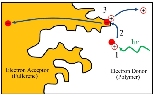
states. ... 6 Figure 1.2: Schematic of a bulk-heterojunction thin film. 1. Light absorption by

the π-conjugated polymer creates an exciton in the polymer phase. 2. Exciton diffusion occurs until an interface between the polymer and fullerene is reached. 3. At the interface, electron injection occurs into the fullerene excited state leaving behind a hole in the polymer HOMO. No longer bound to one another, the electron and hole are now free to migrate to

their respective electrodes. ... 13 Figure 1.3: Schematic of a regenerative DSPEC cell. Photoexcitations in the dye

(D*) undergo electron transfer on an ultrafast timescale into the conduction band (CB) of a nanocrystalline TiO2 particle. This electron is then free to diffuse through the nanocrystalline film until the external circuit is reached where reduction of the electrolyte subsequently occurs at the cathode. Electron injection by the dye results in an oxidized state of the dye (D+)

which then causes oxidation of the electrolyte. ... 16 Figure 1.4: Chemical structure of the dye, [(Ru(bpy)2(4,4’-(PO3H2)2bpy)]2+

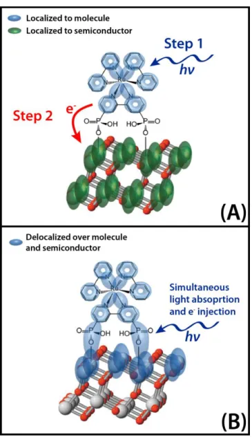
bonded to a nanocrystalline TiO2 particle. ... 18 Figure 1.5: Schematic showing the two mechanisms of molecule-TiO2 electron

injection. Colored ovals represent the spatial locations of excited states in the system. Note that these are shown for illustrative purposes only and do not accurately represent the electronic structure. (A) For this weakly

coupled molecule-TiO2 geometry, excited states are independently localized onto the molecule and TiO2 moieties. Therefore, light absorption creates photoexcitations that are spatially localized to the molecule. Subsequently, after some non zero delay an electron is injected from the molecule excited state to the TiO2 excited state(s). (B) For this strongly coupled molecule-TiO2 geometry, excited states are spatially delocalized over both the molecule and the TiO2. Consequently, light absorption and electron injection should be considered to be the same process (charge transfer

resonance). ... 20 Figure 2.1: The probability of finding the system in state b at time “t” if

xiv

increases, the probability of being found in state b increases as long as the

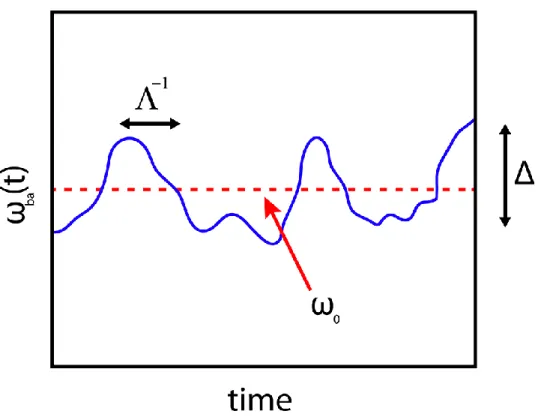
perturbative radiation is on resonance with _ba. ... 31 Figure 2.2: Coupling with the bath causes random fluctuations of the transition

frequency,_babetween the single ground state a and single excited state

b . The transition frequency fluctuates about a mean frequency,₀with a fluctuation amplitude,. Finally, the timescale of bath fluctuations is

governed by the correlation time, 1. ... 37 Figure 2.3: (A) Absorption lineshapes in the two broadening limits. Being in the

homogeneous or “fast-modulation” limit results in Lorentzian lineshapes (black). Being in the inhomogeneous of “slow-modulation” limit results in Gaussian lineshapes (red). (B) The sum of the local inhomogeneous broadening from sub-ensembles that sample only one bath configuration

(black) results in a broad absorption spectrum for the entire ensemble (red). ... 41 Figure 2.4: Donor (D) and acceptor (A) potential energy Born-Oppenheimer free

energy surfaces as described by Marcus theory. Note that it is assumed that the two potential energy surfaces have the same curvature. Therefore, the nuclear configuration, q, is linear in energy.6 In the example shown, a thermally activated electron transfer process is shown where only the solvent contribution (outer-sphere) is considered. First, solvent fluctuations alter the nuclear geometry randomly until the nuclear configuration, q is “correct” for the donor and acceptor surfaces to cross. Once this occurs, the electron transfers from the donor to the acceptor surface, which

subsequently relaxes to the most stable nuclear configuration of the oxidized

donor and reduced acceptor state. ... 46 Figure 2.5: Double sided Feynman diagrammatic approach to time dependent

perturbation theory. Vertical lines represent the density operator, ˆ( )t ( )t ( )t

   where time runs vertically from bottom to top. This particular Feynman diagram represents a 1st order spectroscopic process

between the two states, a and b . ... 52 Figure 2.6: (A) Double sided Feynman diagram corresponding to a 1st order

absorption process. (B) The corresponding energy ladder diagram for the same process showing the excitation of the system from ground state, g to excited state, e through the field matter interaction with field, E1.

Following the propagation interval, t₁ the system radiates the signal field,

ES thus relaxing the system back to the ground state, g . ... 59 Figure 2.7: The six possible double sided Feynman diagrams for a transient

xv

assumed that population initially resides entirely in the ground state, (i.e.,

e g B

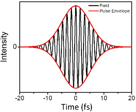
E E k T). ... 62 Figure 3.1: The Gaussian pulse envelope of a ~10 fs laser pulse (red) and the

oscillating real electric field (black). Because this pulse is compressed all

frequencies contained in the pulse bandwidth arrive simultaneously. ... 70 Figure 3.2: Schematic of the oscillating real electric field of a linearly “chirped”

pulse. As time increases, the instantaneous frequency of the pulse increases linearly with time. Note that this has also had the effect of increasing the

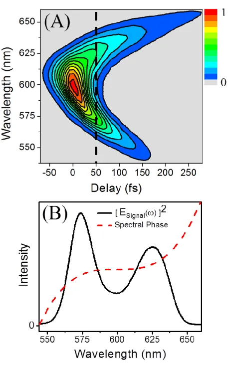
total pulse length in time. ... 74 Figure 3.3: (A) Example pulse spectrogram measured with the FROG technique

utilizing a transient grating beam geometry. Strong quadratic frequency dependence indicates a large amount of third order dispersion in the pulse. (B) Measured signal pulse intensity spectrum at T=50fs with cubic phase overlaid. Note that the phase shown here is shown for illustrative purposes

only. ... 77 Figure 3.4: Schematic of the pulse progression in a simple FROG experiment

utilizing two unique ultrashort pulses. The shorter pulse (black) gates out a portion of the longer linearly “chirped” Gaussian pulse (multicolored) resulting in a measurable signal pulse at each delay, T. Note that the gate pulse only contributes intensity to the signal and does not contribute phase information. Also note that although a two color FROG experiment is shown here, this technique works equally well if the gate pulse and the pulse

to be measured are identical (i.e., spectrally resolved autocorrelation). ... 79 Figure 3.5: Schematic for a simple prism pair pulse compressor used for

compressing ultrashort pulses utilized in Chapters 4-8. Key: M = Mirror, d = tip to tip prism separation, X = Prism position controlling the internal

propagation path length of beams. ... 83 Figure 3.6: Numerical algorithm that adjusts for the effects of TOD in ultrashort

pulses. (A) FROG spectrogram of a FWHM= 2500 cm-1 broadband pulse centered at ~640 nm measured in fused silica as collected. Dotted line represents the frequency dependent “time zero” of the pulse. Arrows

represent the fact that the algorithm forces all frequencies to have a common time zero. (B) Numerically corrected spectrogram of the same pulse. Note that the existence of the “lobes” far from the carrier frequency indicates the fact that the algorithm does not correct for the frequency dependent

instrument response. ... 86 Figure 3.7: Schematic of the group velocity mismatch between the generated

xvi

generation of new signal and idler photons from the leading and trailing edges of the signal and idler pulse, respectively, results in a lengthening of both pulses in time. (B) Noncollinear beam geometries of the signal and idler at a suitable crossing angle, β, allows for group velocity matching in the propagation direction of the signal pulse. As a result, considerably shorter signal and idler pulses can be created than in a collinear beam

geometry. ... 89 Figure 3.8: Schematic of a noncollinear optical parametric amplifier (NOPA)

designed for the creation of femtosecond visible pulses (480-750 nm) at various pulse duration/bandwidths. Key: BS= beam splitter, L= positive focal length lens, -L=negative focal length lens, BBO = Type I β-barium borate crystal, SM=silver coated spherical mirror, ND filter = variable

neutral density filter. ... 92 Figure 3.9: (A) Example spectra of ~20 fs visible pulses generated with a

homebuilt NOPA at various phase matching conditions. (B) NOPA spectra generated at various angles, α, between the pump and seed beams which exhibits the bandwidth tunability of the NOPA setup. Spectral bandwidth shown here ranges from FWHM= 300 cm-1 at the narrowest possible angle

with this setup (blue) to FWHM=5,300 cm-1 (black). ... 93 Figure 3.10: (A) Hollow core fiber setup for spectrally broadening 400 nm

second harmonic pulses from a Ti:Sapphire laser. (B) Spectra of pulses before (black) and after (red) propagation through the hollow core fiber.

Broadening corresponds to decrease in pulse length of about 3.7x. ... 95 Figure 3.11: Top panel exhibits the equilibrium linear absorption spectrum of the

dye, [(Ru(bpy)2(4,4’-(PO3H2)2bpy)]Cl2 adsorbed onto TiO2 nanoparticles. Bottom panel exhibits the TA spectrum of the same system recorded at T=5 ps following 400 nm “pump” excitation. Comparison of the TA spectrum to the equilibrium ground state absorption spectrum in this example clearly exhibits the strong contribution of GSB at shorter wavelengths. At longer wavelengths the ESA signal corresponding to a neutral ligand-metal charge transfer transition dominates.49 ESE is not observed in this sample due to sub-150 fs quenching of excited state population through electron transfer

from the dye to the TiO2 . ... 99 Figure 3.12: Pulse sequence describing a 3rd order spectroscopic experiment such

as transient grating or transient absorption. Pulse centers are defined as _i where the delay between the pulses is given by    _{2 2}and T   _{3 2}. Field matter interactions occur at times t  t₁ t₂ t₃ and t t ₂ t₃ for the first and second “pump” interactions, respectively, tt3 for the “probe”

xvii

Figure 3.13: Beam geometry used in a TG spectroscopy experiment. Green and blue lines represent the “pump” beams and “probe” beams, respectively. The signal beam (red) is radiated in the phase matching direction,

1 2 3

s

k    k k k , which corresponds to a background free direction. ... 102 Figure 3.14: Example of the increase in signal to noise ratio afforded by the use

of heterodyne signal detection over homodyne signal detection. The left panel shows the absolute value of the heterodyne TG signal field of cyclohexane excited and probed with ~15 nJ pulses centered at 266 nm. Data collection time was approximately 5 minutes. The right panel represents the exact same experiment except that the signal was not measured interferometrically. Note that the oscillations shown represent low frequency nuclear motion in cyclohexane. These oscillations are clearly

much more distinct in the heterodyne signal than the homodyne signal. ... 105 Figure 3.15: Absolute value of the TG signal field measured at 530 nm following

400 nm excitation of [(Ru(bpy)2(4,4’-(PO3H2)2bpy)] sensitized TiO2 nanoparticles. Experiments performed with the specialized tensor element ZXZX (gray) exhibit oscillations corresponding to a molecular vibration in TiO2, which provides surprising evidence for strong dye-TiO2 coupling. As these coherences are not observed in the more conventional ZZZZ tensor element (black), these results would not be observable with TA

spectroscopy. See Chapter 8 for a more detailed discussion of these

experiments. ... 110 Figure 3.16: Homebuilt diffractive optic based TG setup used in experiments

described in Chapters 4-8. Key: SM = spherical mirror, CS = quartz

microscope coverslip, WP = wave plate, ND filter = variable neutral density

filter, L = lens, LO = local oscillator, and Pol. = polarizer. ... 112 Figure 4.1: (a) Linear absorption spectrum (black) of the gold cluster. Transient

absorption spectrum 10 ps after excitation with a 530 nm laser pulse (red). The shape of the transmission spectrum ceases to evolve after the first few picoseconds. (b) Transient absorption spectrum at various delay times

following excitation with a 530 nm laser pulse. ... 121 Figure 4.2: (a) Transient absorption signals at selected probe wavelengths

following excitation with a 530 nm laser pulse. The pump and probe wavelengths are indicated in the Figure legend as _pump/_probe. (b)

Transient absorption signals measured with a probe wavelength of 720 nm

after excitation at 530 nm (black) and 660 nm (red). ... 124 Figure 4.3: Electronic relaxation scheme obtained by analysis of femtosecond

xviii

Equilibration of the nuclear structure with the excited state charge

distribution requires 4-5 ps. ... 126 Figure 4.4: Anisotropy [Eq. (2)] in the transient absorption response for three

different pulse configurations. The pump and probe wavelengths are

indicated in the Figure legend as ... 129 Figure 4.5: (a) Transient absorption signal for excitation and probing with a 17

fs, 640 nm laser pulse. (b) Nuclear component of signal obtained by subtraction of exponential decay. (c) Imaginary part of the Fourier transform for nuclear signal component. Solvent (dichloromethane)

resonances are marked with asterisks. The 80 cm-1 vibration of the cluster is

enclosed in a box. ... 131 Figure 5.1: (a) Linear absorption spectrum of Au24Pdat 296 K (black) and 200 K

(red). (b) Linear absorption spectrum of Au25at 296 K (black) and 200 K (red). (c) Photoluminescence spectra of Au24Pd (black) and Au25 (red) at 296K. Au24Pd and Au25 are respectively excited at 400 nm and 530 nm. Periodic structure in the photoluminescence spectrum of Au24Pd in the

700-1000 nm range is an artifact of the measurement. ... 140 Figure 5.2: (a) Real part of transient grating signal spectrum (i.e., equivalent to

conventional transient absorption, ΔA) for Au24Pd (black) and Au25 (red) at 5 ps delay with excitation at 530nm. Signals with negative and positive signs respectively signify the bleach of the ground state and absorption between excited states. (b) Absolute value of the transient grating signal field measured at (b) 630 nm and (c) 700 nm. Fits are obtained with

Equation 5.1. ... 142 Figure 5.3: Time constants (a) ₂ and (b) ₃obtained with a fit of absolute value

of transient grating signal field (see Equation 5.1). The time constants, ₃, in (b) are fit to a Gaussian function (red line) with 695 nm peak and standard deviation of 43 nm. Error bars associated with each time constant are given in each panel. Example fits are shown in Figures 5.2(b) and 5.2(c). All

fitting parameters are tabulated in Appendix A4.2. ... 144 Figure 5.4: Electronic relaxation scheme obtained by analysis of transient grating

experiments. Equilibration of electrons within the metal core occurs in <50 fs, whereas the 500 fs time constant is assigned to internal conversion between core and ligand-localized electronic states. Nuclear relaxation of

the semiring moieties (i.e., ligands) occurs in 25 ps. ... 145 Figure 6.1: Structure of the repeat unit in PNDT-DTPyT. Electron donor (NDT)

and acceptor (DTPyT) functional groups govern the HOMO-LUMO energy gap. The lowest energy electronic transition possesses charge transfer

xix

Figure 6.2: (a) Linear absorbance and (b) fluorescence spectra of pure PNDT-DTPyT films measured at 100K (blue), 200K (red), and 300K (black). In the absorbance spectra, lower temperatures promote an overall red-shift associated with exciton delocalization. The fluorescence line shapes are influenced by both the migration of photoexcitations onto longer segment

lengths and the suppression of thermal fluctuations. ... 157 Figure 6.3: (a) Fit of fluorescence spectrum measured at 300K using Equation

6.2. The blue and red components respectively capture the 0-0 transition and the (effective) vibronic progression of intramolecular modes. Fitting parameters are given in Table 6.1. (b) Frequencies and (c) oscillator strengths corresponding to the lowest energy electronic transitions of PNDT-DTPyT oligomers computed using the ZINDO method. The black squares are obtained directly from the calculations and the red lines are

obtained from fits employing a polynomial expansion. ... 160 Figure 6.4: (a) Fit of linear absorption spectrum at 300K achieved using Equation

6.1. Parameters are adjusted to fit the lowest energy electronic transition shown in red. We postulate a Gaussian line shape (blue) centered at 23300 cm-1 to capture the region of overlapping amplitude near 20170cm-1. (b) Log-normal distribution, G s( ), used to obtain the line shape of the lowest energy transition shown in panel (a). The mean and standard deviation of

( )

G s are respectively 1.4 and 1.2. ... 162 Figure 6.5: (a) Absorptive part of measured TG signal (black) and fit (red) for an

experiment employing 20fs, 16670 cm-1 excitation and detection pulses. All fields possess parallel polarizations. (b) Measured anisotropy (black) and fit (red) for an experiment utilizing the same lasers pulses as panel (a). Noise in the anisotropy at long delay times is caused by the reduction in signal amplitude for the individual tensor elements. All fitting parameters are

given in Table 6.2. ... 165 Figure 6.6: (a) Absorptive part of TG signal measured with excitation at 20400

cm-1_{. Signals are normalized to 1 and plotted on a linear scale. The (b)} ₂ and (c) 3 time constants are obtained by fitting slices of the TG signal in panel (a) at particular detection frequencies. Fitting parameters are given in

Table 6.3. Fits are displayed in Figure A5.13 of Appendix 5. ... 168 Figure 6.7: Experimental evidence that signal components in which PCBM is

both excited and probed can be neglected for PNDT-DTPyT/PCBM

mixtures. (a) Absorbance spectra of PNDT-DTPyT (black) and PCBM (red) are overlaid with the spectrum of the laser (blue). (b) Absorptive part of TG signal for pure PCBM film (black) and a film composed of a 1:1 mixture of PNDT-DTPyT and PCBM (red). These TG experiments employ 20fs,

xx

Figure 6.8: Absorptive parts of TG signals acquired for various weight ratios, PNDT-DTPyT:PCBM. All experiments employ 20fs, 16670 cm-1 excitation and detection pulses. The increase in signal amplitude at long delay times is a signature of electron transfer from PNDT-DTPyT to PCBM. Panels (a) and (b) display the same data on two different time scales. Fitting

parameters are given in Table 6.4. Fits are displayed in Figure A5.14 of

Appendix 5. ... 173 Figure 6.9: Signature of charge separation obtained from fluorescence quenching

experiments. Charge separation causes a decrease in the fluorescence

quantum yield, Q_C, defined by Equation 6.7. ... 175 Figure 6.10: Current-Voltage curves measured for BHJ devices consisting of

different PNDT-DTPyT:PCBM weight ratios. Data was obtained while

illuminating the films with simulated natural sunlight (100 mW/cm2). ... 176 Figure 7.1: Absorbance spectrum of OsII(bpy)3 overlaid with spectra of laser

pulses used in time-resolved experiments... 189 Figure 7.2 (a) Time scale of solvent relaxation calculation with Equation 7.4, _a.

(b) Electron transfer adiabaticity, _ad, obtained with Equation 7.2... 193 Figure 7.3: (a) The diabatic basis associates a three-level system with each

ligand. Couplings, J_e and J_f , are perturbations that do not influence optical resonance frequencies or transition dipoles. (b) Transition dipoles

overlaid on structure of OsII(bpy)3. ... 195 Figure 7.4: Feynman diagrams contributing to transient absorption signals. The

dummy indices a and b sum over the three excited states in the MLCT manifold. The states c correspond to the (three) excited states involving electrons localized on the bipyridine ligands (i.e., bipyridine radicals). In the adiabatic limit, R1, R2, R3, R4, R1* and R2* are unrestricted in that terms in which ab contribute, whereas the nonlinearities are limited to terms

where ab in the diabatic basis. ... 196 Figure 7.5: Transient absorption signals in diabatic basis for S_ZZZZ

 

and S_ZZZZ

 

panels (a) (black); (b) (red); and (c) (blue). ... 201 Figure 7.6: Electronic structure in adiabatic basis found with D3 symmetry.

xxi

respectively associated with the MLCT band and bipyridine radical

electronic states. ... 203 Figure 7.7: (a) Sequences with pairs of field-matter interactions occurring with

diabatic MLCT transitions localized to different ligands, ab, are forbidden. (b) Pairs of field-matter interactions with different MLCT transitions, ab, are allowed in the (delocalized) adiabatic basis. (c) Field-matter interaction sequence for the R4 diagram. The transient absorption anisotropy of R4 depends on relative MLCT transition dipole orientations

only in the adiabatic basis. ... 205 Figure 7.8: Schematic depicting the effect of the pump laser frequency on

dynamics in the transient absorption anisotropy. A wavepacket initiates on the upper quasi-adiabatic surface, relaxes to the avoided crossing with time

constant et1, then depolarizes as electrons localize on the individual ligands. ... 207 Figure 7.9: Transient absorption signals measured with ZZZZ (black) and ZZXX

(red) tensor elements and pump/probe wavelengths: (a) 680nm/610nm; (b) 645nm/645nm; (c) 610nm/610nm; (d) 570nm/570nm. Transient absorption is defined as the real part of the experimentally measured transient grating signal field, where the positive sign represents absorption between excited

states. ... 212 Figure 7.10: Transient absorption anisotropies calculated using the data in Figure

7.9 with the pump/probe wavelengths: (a) 680nm/610nm; (b)

645nm/645nm; (c) 610nm/610nm; (d) 570nm/570nm. Fitting parameters

are given in Table 7.1... 214 Figure 7.11: Transient absorption anisotropies obtained with excitation at 680

nm and a broadband probe pulse with a spectrum spanning the 500-750 nm

range. Delay times, T, are given in the Figure legend. ... 216 Figure 8.1: (a) Absorbance spectra of catechol in aqueous solution (red) and

adsorbed to a TiO2 nanocrystalline film (blue). (b) Absorbance spectra of the ruthenium complex in aqueous solution (red) and adsorbed to a TiO2 nanocrystalline film (blue). The absorbance spectrum of a neat TiO2 film is

displayed in both panels (black). ... 227 Figure 8.2: Absolute value of TG signals acquired under the ZXZX tensor

element with “pump” (E₁ and E₂) and probe (E₃) pulses centered at 400nm and 525nm, respectively. Signals acquired for the molecule-TiO2

composites are fit with a red line, whereas those obtained for the neat TiO2 films are fit with a blue line. All samples including the neat TiO2 films are in aqueous solutions (cf., Appendix A7). The inset of panel (a) illustrates the orientations of the four electric field polarizations involved in the ZXZX

xxii

Figure 8.3: Absolute value of TG signals acquired under the ZXXZ tensor element for a neat TiO2 film with “pump” (E1 and E2) and probe (E3) pulses centered at 400nm and 525nm, respectively. The inset illustrates the orientations of the four electric field polarizations involved in the ZXXZ tensor element. Fitting components are given in Table 8.1. (b) Spontaneous Raman spectrum of the same TiO2 film obtained with an excitation

wavelength of 633nm. This measurement suggests that the vibrational

coherence detected by TG is associated with the ground electronic state. ... 231 Figure 8.4: The amplitude of the vibrational coherence in the ~142cm-1 mode

increases with the displacement in the potential energy minima associated with the ground and excited electronic states, . We assign the vibrational motions detected in this work to the ground electronic states of the

composite molecule-TiO2 systems. ... 233 Figure A2.1: Time domain picture of a measured TG interferogram at a single

pulse delay. The local oscillator intensity is removed from the measured signal through the use of an apodization function (red) which is centered over the positive signal peak. Following multiplication with the apodization function, the time domain TG signal is Fourier transformed back to the

frequency domain... 246 Figure A3.1: Transient absorption signals (black) and fits (red) at selected probe

wavelengths following excitation with a 530 nm laser pulse. The pump and probe wavelengths are given in each panel as pump_/probe_{. Parameters} corresponding to the fits are defined by Equation 4.1 and Table 4.1 of

Chapter 4. ... 247 Figure A3.2: Transient absorption measurements corresponding to Figure 4.5 in

Chapter 4. Pulse configurations are: (a) 530nm pump/530 nm probe; (b) 530nm pump/720 nm probe; (c) 660nm pump/720 nm probe. Black and red lines respectively represent measurements performed with parallel and

perpendicular pump and probe polarizations. ... 248 Figure A5.1: The alkane side chains of PNDT-DTPyT branching from the atoms

indicated with an asterisk are replaced methyl groups in order to manage computational expense in both the DFT geometry optimization and ZINDO electronic structure calculations. Removal of these aliphatic groups has

little effect on the lowest energy electronic transitions. ... 253 Figure A5.2: Optimized geometry as calculated by Density Functional Theory of

the PNDT-DTPyT repeat unit. The two carbon atoms labeled with asterisks indicate where the linkage between units occurs. This geometry is used as input for the ZINDO electronic structure calculations discussed in Chapter

xxiii

Figure A5.3: Optimized geometry as calculated by Density Functional Theory of the PNDT-DTPyT dimer. This geometry is also used as input for the

ZINDO electronic structure calculations discussed in Chapter 6.1. ... 255 Figure A5.4: Calculated structure of the oligomer of PNDT-DTPyT containing

three repeat units. This geometry is used as input in the ZINDO electronic structure calculations discussed in Chapter 6.1. Note that this structure is not a result of a DFT geometry optimization, but is mathematically

calculated assuming that the trans linkage shown in Figure A5.3 is periodic. ... 257 Figure A5.5: Calculated structure of the oligomer of PNDT-DTPyT containing

four monomer segments. This geometry is used as input in the ZINDO electronic structure calculations discussed in Chapter 6.1. Note that this structure is not a result of a DFT geometry optimization, but is

mathematically calculated assuming that the trans linkage shown in Figure

A5.3 is periodic. ... 257 Figure A5.6: Calculated structure of the oligomer of PNDT-DTPyT containing

five monomer segments. This geometry is used as input in the ZINDO electronic structure calculations discussed in Chapter 6.1. Note that this structure is not a result of a DFT geometry optimization, but is

mathematically calculated assuming that the trans linkage shown in Figure

A5.3 is periodic. ... 258 Figure A5.7: Calculated structure of the oligomer of PNDT-DTPyT containing

six monomer segments. This geometry is used as input in the ZINDO electronic structure calculations discussed in Chapter 6.1. Note that this structure is not a result of a DFT geometry optimization, but is

mathematically calculated assuming that the trans linkage shown in Figure

A5.3 is periodic. ... 258 Figure A5.8: Calculated structure of the oligomer of PNDT-DTPyT containing

seven repeat units. This geometry is used as input in the ZINDO electronic structure calculations discussed in Chapter 6.1. Note that this structure is not a result of a DFT geometry optimization, but is mathematically

calculated assuming that the trans linkage shown in Figure A5.3 is periodic. ... 259 Figure A5.9: Calculated structure of the oligomer of PNDT-DTPyT containing

eight repeat units. This geometry is used as input in the ZINDO electronic structure calculations discussed in Chapter 6.1. Note that this structure is not a result of a DFT geometry optimization, but is mathematically

calculated assuming that the trans linkage shown in Figure A5.3 is periodic. ... 259 Figure A5.10: Calculated structure of the oligomer of PNDT-DTPyT containing

xxiv

not a result of a DFT geometry optimization, but is mathematically

calculated assuming that the trans linkage shown in Figure A5.3 is periodic. ... 260 Figure A5.11: Ground state absorbance of thin films of PNDT-DTPyT doped

submerged in gaseous I2 (cf., Chapter 6.3). The concentration of the cation, PNDT-DTPyT+, increases as the exposure time increases. Although the spectrum of the pure cation is not obtained, this series of measurements shows that the cation absorbs in the visible wavelength range. Note that the absorbance increases at frequencies less than 12500cm-1 and greater than 18000cm-1. Therefore, the cation, along with the PCBM anion, can

contribute to the excited state absorption nonlinearities probed in this work. ... 263 Figure A5.12: Fluorescence spectra are fit at (a) 200K and (b) 100K with a sum

of two Gaussian functions. The reorganization energy,  ₁2/ 2k T_B , is estimated using the line width of the nominal 0-0 transition (i.e., higher energy peak), where ₁ is the standard deviation of the function. Fits conducted at 200K and 100K yield ₁=524 cm-1 and ₁=473 cm-1,

respectively. ... 264 Figure A5.13: Real part of measured transient grating signals (black) and fits

(red) for pure PNDT-DTPyT films. Signals are acquired with all fields possessing parallel polarizations, S T

 

scales. The detection frequency is given in each panel. ... 265 Figure A5.14: Real part of measured transient grating signals (black) and fits

(red) obtained using Equation 6.4. Signals are acquired with all field possessing parallel polarizations, S T

 

log scales. The weight ratios, PNDT-DTPyT:PCBM, is given in each panel. ... 266 Figure A6.1: Feynman diagrams for R3 and R4 terms contributing to the GSB

signal component ... 273 Figure A6.2: Feynman diagrams for R1 and R2 terms contributing to the ESE

signal component ... 274 Figure A6.3: Feynman diagrams for R1 and R2 terms contributing to the ESA

signal component ... 275 Figure A6.4: Feynman diagrams for ICR1* and ICR2* terms contributing to the

ESA signal component ... 275 Figure A6.5: Feynman diagrams for R3 and R4 terms contributing to the GSB

xxv

Figure A6.6: Feynman diagrams for R1 and R2 terms contributing to the ESE

signal component ... 278 Figure A6.7: Feynman diagrams for R1* and R2* terms contributing to the ESA

signal component ... 279 Figure A6.8: Feynman diagrams for ICR1* and ICR2* terms contributing to the

ESA signal component ... 279 Figure A6.9: Transient absorption signals obtained as the real part of transient

grating signal fields at pulse delay, T: (a) 0.10 ps; (b) 0.25 ps; (c) 0.45 ps; (d) 0.75 ps; (e) 3.0 ps. These data are used to calculate the anisotropies

shown in Figure 7.11... 281 Figure A7.1: Home-made cuvette used to contain dye-sensitized films during

transient grating experiments. ... 285 Figure A7.2: Dye sensitized TiO2 films are held in a home-made cuvette during

transient grating experiments and oscillated in the plane of the film with a

xxvi

LIST OF ABBREVIATIONS AND SYMBOLS

A acceptor molecule

A- reduced acceptor molecule

Å angstrom

( )

A

A  acceptor molecule absorption spectrum

( )

  polarizability

Au gold

b Kuhn monomer length

BBO β-barium borate BHJ bulk heterojunction

c speed of light

CB conduction band

CCD charge coupled device

(1)

n

c first order coefficient of state “b”

CS quartz coverslip

( )

C T correlation function

( ) ( )

n

  susceptibility at nth order

xxvii

D* photoexcited dye or photoexcited donor molecule D+ oxidized dye or donor molecule

DFT density functional theory

DSPEC dye sensitized photoelectrochemical cell A

d_ specific vibrational nuclear coordinate

 fluctuation in energy gap due to interactions with surroundings

E(t) electric field

e- electron

EET electronic energy transfer ESA excited state absorption ESE excited state emission ET electron transfer

eV electron volt

ΔE† energy activation barrier  extinction coefficient

( )

D

F  donor molecule fluorescence spectrum

F fluence

 

f s oscillator strength

xxviii FRET fluorescence resonance energy transfer FROG frequency resolved optical gating

fs femtosecond

FWHM full width half maximum G

 free energy change

( )

G s log normal distribution

( )

g t line broadening function





G t w Gaussian instrument response function

( )t_n

G Green Function

GSB ground state bleach GVD group velocity dispersion

 _{damping constant for line broadening function}

h Planck’s constant

reduced Planck’s constant (h/ 2π)

Coul

H coulombic coupling

DA

H energy gap Hamiltonian (H_AH_D)

el ph

H  electron-phonon coupling

xxix

η (%) photovoltaic power conversion efficiency

DA

J dipole-dipole coupling between donor and acceptor molecules

Jsc short circuit current

k rate

kB Boltzmann’s constant

n

k _{wavevector of pulse “n”}



( )

L  absorption lineshape LO local oscillator

LUMO lowest unoccupied molecular orbital 1



 correlation time of solvent fluctuations  reorganization energy or wavelength

M number of stabilizing ligands MPC monolayer protected cluster MLCT metal to ligand charge transfer

 

M t

solvation correlation function

μm micrometer

N number of metallic atoms in a nanocluster or number of monomers

A

xxx ND neutral density

nm nanometer

NOPA noncollinear optical parametric amplifier

n* number of electrons available in a nanocluster OHD optical heterodyne signal detection

OPA optical parametric amplifier OPG optical parametric generation OPV organic photovoltaic

 angular frequency

0

 carrier frequency

vib

 vibrational frequency

( )

n

P t probability of residing in state “n” at time t.

( )

n

P kT thermal population of state “n”

( )n

P polarization of nth order

PCBM phenyl-C61-butyric acid methyl ester

ps picosecond

q collective nuclear coordinate

DA

r intermolecular distance between donor and acceptor molecules

( )

xxxi

ˆ( )t

 time dependent density operator

C

Q fluorescence quantum yield

( )

R t response function term

R mean end to end distance in a polymer chain ( )

S T signals measured with parallel pump and probe polarizations

( )

S T_ signals measured with orthogonal pump and probe polarizations ( )

( )

n

S t response function of nth order

SM spherical mirror

( )t

 wavefunction

 absorption cross section

T temperature (or time interval) TA transient absorption

TAA transient absorption anisotropy TDPT time dependent perturbation theory TG transient grating

( )

group

t  group velocity

TOD third order dispersion ( )t

xxxii

( )

  spectral phase

 transition dipole

ˆ( )t

 dipole operator

ˆ ( )_I

V t time dependent interactive perturbation

ba

V coupling between states “a” and “b”

Voc open circuit voltage

 frequency

A

v number of valence electrons

wp wave plate

( )t

 Gaussian envelope function

z charge

CHAPTER 1. INTRODUCTION

1.1. MOTIVATION

On the smallest length scales the world is a very complicated place. Even in seemingly simple macroscopic systems, the underlying physical processes occurring can be quite complex and difficult to ascertain. For example, although water is one of the simplest chemicals and probably has been studied more than any other, we still do not have a complete understanding of some of its most basic properties.1,2 For more complex systems with many degrees of freedom (e.g., macromolecules, synthetic devices, etc.) obtaining an exact picture of what occurs on the molecular scale is a monumental challenge. In most cases, we will probably never obtain an exact understanding and must therefore content ourselves with a partial understanding through the use of models.

2

This dissertation is concerned with probing the mechanisms of energy and charge transfer following photoexcitation in a variety of synthetic systems. These systems range from applied materials synthesized for use in solar energy conversion (conjugated polymers and transition metal polypyridyl complexes) to materials synthesized for more fundamental research (“quantum-sized” gold nanoclusters). With the solar energy materials, it is absolutely essential to obtain a deep understanding of the energy and charge transfer mechanisms as these processes are strongly linked to the overall efficiency of a working device. On the other hand, knowledge of energy and charge transfer mechanisms in less applied systems such as gold nanoclusters is equally as important due to the fact that on a fundamental level, all mechanistic models are related. Consequently, furthering the understanding of energy and charge transport in one system helps one understand these processes in all systems.

All quantum mechanical mechanistic energy and charge transfer rate models are in effect derivatives of the famous rate equation developed by Dirac and Fermi in the first half of the 20th Century.3,4 This rate equation, now known as “Fermi’s Golden Rule,” calculates the transition rate between two or more coupled states following some external perturbation (e.g., interaction with an electromagnetic field). Fermi’s Golden Rule is extremely powerful because it describes the rates of change for essentially all possible situations and mechanisms. This flexibility is possible because one needs only to change the coupling parameter in the equation (i.e., the perturbative Hamiltonian) to match the specifics of the system/mechanism being modeled.

3

herein are the Marcus theory of electron transfer5 and the Förster Resonance Energy Transfer theory.6 The former is used extensively in the study of both intramolecular and intermolecular electron transfer mechanisms in osmium and ruthenium polypyridyl complexes both bound and unbound to TiO2 semiconductornanoparticles. Discussions of these studies are included in Chapters 7 and 8 along with a derivation of Marcus theory shown in Chapter 2.2.3. Förster theory is used prominently in the study of energy transfer mechanisms in the form of “hopping” of photoexcitations between chains of a newly synthesized π-conjugated polymer for use in solar energy collection. This study is discussed in Chapter 6 and a derivation of Förster theory is shown in Chapter 2.2.2. Studies of energy transfer mechanisms in gold nanoclusters are included in Chapters 4 and 5. In these systems the primary mechanism of energy transfer observed is internal conversion between spatially localized excited states. Although the laws governing internal conversion can also be shown to be a derivative of Fermi’s Golden Rule where the coupling parameter is described by the nuclear kinetic energy operator,7-9 the mathematics are considerably more complicated than in the other examples and a derivation is not included in this dissertation.

4

attoseconds for more energetic spectroscopies (e.g., X-Rays).14 Although providing equivalent information to more conventional “pump-probe” techniques such as transient absorption, the transient grating technique utilized in this dissertation has several advantages over the former including background free signals and the ability to use extremely low laser fluences. In addition, the use of multiple laser beams to excite and probe the samples allows for direct control over all field matter interactions with the sample (e.g., control of polarizations). As will be demonstrated in Chapter 8, this is an extremely valuable advantage, which allows one to probe charge transfer dynamics that would otherwise be unobservable.

1.2. GOLD NANOCLUSTERS

1.2.1. Bulk and Quantum-Sized Regimes

5

Perhaps the most interesting aspect of gold nanoparticles, however, is the fascinating dependence exhibited by the electronic and optical properties on the size and shape of the nanoparticle. In general, there are two main size regimes to consider. For “large” gold nanoparticles in the 3-100 nm size range, the absorption spectra are broad and featureless; consisting primarily of a surface plasmon band.16,17,25,26 That is, light absorption is the result of interactions between photons and the 6s conduction band electrons of the surface gold atoms. This is analogous to the interactions that occur in the bulk material with one important exception being that the bandgap between the valence and conduction bands is considerably larger in nanoparticles than in the bulk material. As the size of the nanoparticle increases, the bandgap decreases; eventually matching the electronic structure of bulk gold.

6

CH2CH2Ph moieties not included in Figure 1.1(A) for clarity. Full spectroscopic studies of this particular cluster and the analogous cluster, Au24Pd(SR)18- are described in detail in Chapters 4 and 5, respectively. Here it is sufficient to say that the peaks observed in the absorption spectrum correspond to the lowest energy electronic transitions between states localized to the Au13 core structure.

7 1.2.2. Superatom Model

If the concepts governing the absorption spectra of gold nanoclusters are comparable to that of molecules, then the rules that govern the stability of gold nanoclusters can be said to atomistic in nature. As taught in general chemistry courses, the electronic configuration of an atom is determined by the Aufbau principle in which an atom’s atomic orbitals are filled up successively with electrons according to the most stable configuration. Filled and half filled angular momentum “shells” are especially stable, which leads to a specific order in which the “shells” are filled (i.e., 2 2 6 2 6

1 2s s 2p 3 3s p ...).

In an analogous manner, the Superatom model predicts the stability of metallic nanoclusters by modeling their electronic structures as a building up of electrons in a sequence of angular momentum “shells” of a “jellium sphere.”33,36,43-45

The sequence of angular momentum “shells” resembles that of individual atoms and is given as

2 6 10 2 14 6 18 10 2 22

1S 1P 1D 2 1S F 2P 1G 2D 3 1S H ...

             

              (1.1)

where each set of brackets encloses a single “shell,” the letters represent the character of the angular momentum of a “sub-shell”, the superscripts refer to the maximum number of electrons that can be contained in each “sub-shell”, and the numbers in front of the letters represent the principle quantum number.36 According to the Superatom model, filled shells correspond to maximum stability; therefore a given nanocluster will be stable if the total number of available electrons in the nanocluster,n*, is equal to the following36

*

2, 8, 18, 34, 58, 92, 138, ....

8

The number of electrons available is proportional to the number of metal atoms included in the nanocluster and is given by the following expression

*

A

n Nv Mz (1.3)

where N is the number of metal atoms included in the nanocluster, v_A is the number of valence electrons in each atom, M is the number of stabilizing ligands attached to the nanocluster, andz is the net charge of the nanocluster.36

The Superatom model has been very successful at predicting and explaining the stability of nanoclusters.44-49 In the context of this dissertation, it can readily explain the stability of the gold nanocluster, Au25(SR)18-. For this nanocluster, twelve of the twenty five gold atoms are located in the semiring moieties, and thus should not be included in Equation 1.3. The Au13 core of the nanocluster contains the remaining gold atoms, thereforeN13. Each gold atom contributes a single valence electron (i.e.,6s1), thusv_A 1. Each semiring moiety is considered to be a single ligand, therefore makingM 6. Finally, as the charge of the nanocluster is negative, z 1. If one inserts these parameters into Equation 1.3, the number of electrons available, n* is equal to 8, which corresponds to a stable filled

2 6 1S 1P

   

9 1.3. ORGANIC PHOTOVOLTAIC MATERIALS

1.3.1. Organic Semiconducting Polymers

Currently, solar energy collection technologies are on the brink of but not quite efficient/cheap enough compete commercially with terrestrial energy sources. There is a great deal of emphasis being put on this problem in the scientific community, however, and new advances in concepts and technology are constantly closing the gap. One promising avenue of solar energy technology research deals with the use of organic photovoltaic devices (OPV) whose functionality is based on the semiconducting properties of π-conjugated polymers. Although currently yielding device efficiencies ( 10%) notably lower than “conventional” inorganic solid state junction semiconductor photovoltaics, OPVs have several advantages over the former including: significantly lower manufacturing costs, molecular-level customization, and thin film flexibility.50,51

The backbone of a π-conjugated polymer chain consists of an uninterrupted progression of unsaturated carbon atoms. Each carbon atom is in a 2

10

referred to as the valence and conduction bands for the HOMO and LUMO states, respectively. The bandgap of π-conjugated polymers is typically low (~1-4 eV), making the corresponding optical transition in the visible-NIR spectral region.53 Furthermore, because functionalization of the polymer chain strongly affects the delocalization properties of the polymer, one has the ability to fine-tune the bandgap to optimally match the solar spectrum by “simply” altering the chemical structure of the chains.52-54

11

exciton into free charges.51,59 This type of device is referred to as a bulk heterojunction and will be discussed in the next section.

1.3.2. Bulk Heterojunction Films

As discussed in the previous section, low energy photoexcitations in π-conjugated polymers consist of excitons and not free charge carriers. In order to generate the free charges required for photovoltaic devices to function, one must introduce an electron accepting material to the system in order to dissociate excitons into unbound electrons and holes. Since the observation of sub-picosecond electron transfer from π-conjugated polymers to fullerenes in the 1990’s,60,61 fullerenes and their functionalized derivatives (e.g., PCBM) have become the most widely used electron accepting materials in OPV devices. The simplest manner in which to contact the two materials together in a device is in a bilayer configuration, where there are simply two layers of pristine π-conjugated polymer and fullerene in contact with one another.62 As excitons in π-conjugated polymers typically exhibit a diffusion length of only ~10 nm before undergoing radiative/nonradiative relaxation, polymer film thicknesses in bilayer devices cannot exceed this length.50,63-70 Unfortunately, this thickness is considerably less than the average optical absorption depth of π-conjugated polymers (~100 nm), which severely limits the amount of sunlight that can be absorbed.50

A considerably more efficient device design is the bulk heterojunction (BHJ) thin film. A bulk heterojunction is simply a random microscopically interpenetrating mixture of π-conjugated polymer and fullerene phases formed by self-organized phase separation.51,59

12

materials is considerably less than in bilayer devices, therefore increasing the number of excitons that are able to diffuse to a polymer/fullerene interface and undergo electron transfer. Additionally, the thickness of BHJ films is not limited by the exciton diffusion length and thicker films can be prepared that maximize light absorption. As of today, BHJs are the state of the art for OPV devices, and photo conversion efficiencies in the range of 3-10% have been reported.71-80

13

Figure 1.2: Schematic of a bulk-heterojunction thin film. 1. Light absorption by the π-conjugated polymer creates an exciton in the polymer phase. 2. Exciton diffusion occurs until an interface between the polymer and fullerene is reached. 3. At the interface, electron injection occurs into the fullerene excited state leaving behind a hole in the polymer HOMO. No longer bound to one another, the electron and hole are now free to migrate to their respective electrodes.

1.4. DYE–SENSITIZED PHOTOELECTROCHEMICAL CELL

1.4.1. Introduction

14

type and purpose of the photoelectrochemical cell. The photo-anode, (typically an n-type inorganic semiconductor) absorbs any photons whose energy exceeds the semiconductor’s bandgap to create unbound electron-hole pairs.81 The electrons diffuse through the semiconductor and into an external circuit connected to the cathode. The holes diffuse to the semiconductor-electrolyte interface, where one of two things will happen depending on the type of photoelectrochemical cell. In a regenerative cell, the hole oxidizes an electrolyte molecule which then migrates to the cathode. Upon arriving at the cathode, the oxidized electrolyte molecule is reduced back to its original state by an electron which has traveled through the external circuit. This process is constantly repeated thus creating an external current which can be used to perform useful work.81 The other type of photoelectrochemical cell is referred to a photosynthetic cell. Photosynthetic cells are identical to regenerative cells in all respects except for the fact that the electrolyte consists of more than one redox system that do not regenerate. One redox system is reduced by interaction with the photoelectrons at the cathode, thus creating a useful chemical product (e.g., H O₂ eH₂) which can be collected and stored for further use. The other redox system is oxidized at the semiconductor anode by the holes to again create a useful product (e.g., H O₂ O₂e).

15

and charge carrier generation processes. This is accomplished by sensitizing the semiconductor anode with a chemical dye whose absorption spectrum better matches the solar spectrum.81,86-88 Although dye sensitization is certainly not a new concept, original designs were limited by low light harvesting efficiencies due to the belief that only flat semiconductor surfaces should be used.89,90 The invention of the “Grätzel Cell” by Michael Grätzel and coworkers in 1991 was a revolution in dye sensitized photoelectrochemical cell design and now represents the most famous and one of the more efficient (7-8%) and cost-effective designs.88 In the Grätzel Cell, in order to maximize light absorption, the flat semiconductor anode was replaced with a mesoscopic thin film (~10 µm thick) of crystalline TiO2 semiconductor nanoparticles. This ultimately increased the surface area available for dye adsorption by orders of magnitude relative to a flat surface, while surprisingly still retaining a large charge carrier mobility in the TiO2.86,88 Nearly all subsequent dye sensitized photoelectrochemical (DSPEC) cells designs are based on this concept.

16

Figure 1.3: Schematic of a regenerative DSPEC cell. Photoexcitations in the dye (D*) undergo electron transfer on an ultrafast timescale into the conduction band (CB) of a nanocrystalline TiO2 particle. This electron is then free to diffuse through the nanocrystalline film until the external circuit is reached where reduction of the electrolyte subsequently occurs at the cathode. Electron injection by the dye results in an oxidized state of the dye (D+) which then causes oxidation of the electrolyte.

1.4.2. Ruthenium Polypyridyl Complexes

17

In ruthenium polypyridyl complexes the electronic transition responsible for the visible absorption is a metal to ligand charge transfer process (MLCT) from the central ruthenium atom to one of the ancillary ligands.86 Functionalizing these ancillary ligands (typically bipyridine or terpyridines) allows one to alter the energy levels of the MLCT states therefore giving synthetic chemists the ability to “tune” the electronic properties of the complexes to suit one’s specific requirements.86

18

Figure 1.4: Chemical structure of the dye, [(Ru(bpy)2(4,4’-(PO3H2)2bpy)]2+ bonded to a nanocrystalline TiO2 particle.

1.4.3. Electronic Structure at Molecule-TiO2 Interfaces

The first and arguably the most important step of any working DSPEC cell is the absorption of a photon by the dye molecule and subsequent electron injection into the conduction band of the semiconductor nanoparticle. While the ensuing steps are clearly also important, it is the efficiency of this electron injection process that directly governs the availability of free charge carriers in a device. For this reason, a great deal of research has been performed in order to further the understanding of the mechanism(s) of electron injection in molecule-sensitized semiconductor systems.

19

explained by an electron injection model developed by Marcus and Gerischer in the 1960-70s in which the photon absorption and electron injection steps are described as sequential.5,98,99 That is, light absorption by the sensitizing molecule yields photoexcitations in excited states that are spatially localized in the molecule. After some finite delay, an electron is then injected from the molecule into the TiO2 conduction band. This process is illustrated schematically in Figure 1.5(A). The rate of injection in this model is described by Marcus theory and is determined primarily by the molecule-TiO2 coupling strength and the density of states in the TiO2 conduction band at the energy of the molecule’s excited state.

20

techniques will exhibit evidence for this surprising result even for the nominally weakly coupled system, [(Ru(bpy)2(4,4’-(PO3H2)2bpy)]2+ adsorbed on TiO2.

21 1.5. STRUCTURE OF DISSERTATION

As aforementioned, this dissertation is concerned with examining mechanisms of energy and charge transport in a variety of synthetic systems. Chapter 2 reviews the theoretical framework needed to describe these mechanisms. Starting with the standard form of Fermi’s golden rule, a reduced description of the rate law will be presented that is more suitable for the condensed phase systems studied herein. Derivations of Förster theory, Marcus theory, and absorption lineshapes from this reduced description are included to demonstrate its versatility. Finally, a discussion of optical response theory in the context of time dependent perturbation theory provides the groundwork for understanding spectroscopic experiments in this dissertation. Diagrammatic time dependent perturbation theory is introduced as well as four-wave mixing signal components.

22

A primarily spectroscopic study on the newly synthesized low band gap π-conjugated polymer, PNDT-DTPyT is presented in Chapter 6. Transient grating experiments probing the energy and electron transfer mechanisms of both pure polymer thin films and polymer-PCBM bulk heterojunction thin films are discussed in detail. Results are found to correlate with overall photoconversion efficiencies for devices prepared in an identical manner. Chapter 7 presents a study on intramolecular electron transfer mechanisms in the prototypical transition metal polypyridyl complex, OsII(bpy)3. Transient absorption anisotropy is developed as a new experimental technique in which to ascertain the adiabaticity of electron transfer mechanisms; a property that is notoriously difficult to determine experimentally.

Finally, Chapter 8 presents specialized transient grating experiments probing the electron injection mechanism of the dye sensitized TiO2 nanocluster system, [(Ru(bpy)2(4,4’-(PO3H2)2bpy)]2+/TiO2. Results provide surprising evidence of a large sub-ensemble of the system exhibiting strong dye-TiO2 coupling (i.e, charge transfer character) even with the nominally weakly coupled phosphonate linkers. These conclusions are verified with identical experiments on a strongly coupled system, catechol-TiO2. The specialized technique used in this study is suggested as a simple and direct method to probe the “average” charge transfer character of a given system.