TREE ORIENTED DATA ANALYSIS
Sean Skwerer
A dissertation submitted to the faculty at the University of North Carolina at Chapel Hill in partial fulfillment of the requirements for the degree of Doctor of Philosophy in the Department of Statistics
and Operations Research.
Chapel Hill 2014
ABSTRACT
Sean Skwerer: Tree Oriented Data Analysis (Under the direction of J. S. Marron and Scott Provan)
Complex data objects arise in many areas of modern science including evolutionary biology, nueroscience, dynamics of gene expression and medical imaging. Object oriented data analysis (OODA) is the statistical analysis of datasets of complex objects. Data analysis of tree data objects is an exciting research area with interesting questions and challenging problems. This thesis focuses on tree oriented statistical methodologies, and algorithms for solving related mathematical optimization problems.
This research is motivated by the goal of analyzing a data set of images of human brain arteries. The approach we take here is to use a novel representation of brain artery systems as points in phylogenetic treespace. The treespace property of unique global geodesics leads to a notion of geometric center called a Fr´echet mean. For a sample of data points, the Fr´echet function is the sum of squared distances from a point to the data points, and the Fr´echet mean is the minimizer of the Fr´echet function.
ACKNOWLEDGEMENTS
My success in completing the requirements for a PhD could not have happened without contribu-tions from many individuals through mentorship, teaching, friendship and support.
The two most important figures are my advisers Steve and Scott.
Steve has been a source of inspiration and clarity during this research project. I admire his ability to bring researchers together.
Scott has contributed enormously through his tireless patience and commitment to his students. I am grateful for his dedication.
Ezra Miller has been an unofficial mentor to me. His great knowledge of mathematics and affable character have lead me to pursue many discussions.
In my memory, there are two teachers who have had a profound impact on my interest in mathematics, and thus to whom I owe my career path. I am grateful to Gabor Pataki who inspired me as a Freshmen at UNC-CH in an elementary course called Introduction to Decision Sciences. I am also grateful to Gabor for encouraging me to become a PhD student. I am grateful to Gene Tournoux my pre-calculus instructor at Shaker Heights Highschool who nurtured skills which formed a basis for my approach to mathematical problem solving from highschool through graduate school.
I am grateful to my parents for raising me in a home were learning is valued.
PREFACE
This thesis is based on collaborative work with my advisors J. S. Marron and Scott Provan in the domain of tree oriented data analysis. Chapter 1, which provides an overview of tree oriented data analysis and background material, is the original work of the student.
Chapter 2, which describes the treespace Fr´echet mean optimization problem, and related theory and methods, is the original work of the student. Section 2.1 provides an overview and discussion of the problem, and these perspectives are an original contribution by the student. Section 2.2 and section 2.3 focus on summarizing existing theory and methodology. Sections 2.4 and 2.5 contain novel unpublished research by the student.
Chapter 3 summarizes data analytic results. This analysis was conducted by the student, with one exception, the result attributed to Megan Owen in Section 3.1. The discussion of Fr´echet mean degeneracy in this chapter is an extension of research from a paper written by this student in collaboration with a number of authors (see reference) (Skwerer et al., 2014).
Chapter 4 contains novel theoretical analysis by the student. Section 4.1 contains background material. Section 4.2 provides a summary of related research that the student contributed to as part of a collaborative research group. Section 4.3 contains an original presentation of basic definitions and novel unpublished results by the student. Section 4.4 contains the main result of the chapter which is unpublished research by the student.
TABLE OF CONTENTS
LIST OF TABLES . . . x
LIST OF FIGURES . . . xi
LIST OF ABBREVIATIONS AND SYMBOLS . . . .xiii
CHAPTER 1: INTRODUCTION . . . 1
1.1 Dissertation Overview . . . 1
1.2 Phylogenetic trees and BHV treespaces . . . 3
1.2.1 Graphs and trees . . . 3
1.2.2 Phylogenetic trees . . . 3
1.2.3 Construction of BHV Treespaces . . . 4
1.3 Brain artery data . . . 5
1.4 Mapping Brain Artery Systems to BHV treespace . . . 6
1.4.1 Correspondence . . . 6
1.5 Other approaches to tree oriented data analysis . . . 7
1.5.1 BHV treespace geodesics . . . 7
CHAPTER 2: Methods for Fr´echet Means in Phylogenetic Treespace . . . .15
2.1 Introduction. . . .15
2.1.1 Fr´echet means in BHV treespace . . . .15
2.1.1.1 Problem Discussion . . . .16
2.2 Global search methods . . . .20
2.2.1 Inductive means . . . .20
2.2.2 Cyclic Split Proximal Point Algorithm . . . .21
2.3 Vistal cells and squared treespace . . . .21
2.5 Interior point methods for optimizing edge lengths . . . .34
2.5.0.1 Optimality Qualifications . . . .35
2.5.1 A damped Newton’s method . . . .36
2.5.1.1 Newton steps . . . .36
2.5.1.2 Choosing a step length . . . .37
2.5.1.3 Initialization . . . .38
2.6 Updating Geodesic Supports . . . .40
2.6.0.4 Setup and notation . . . .40
2.6.0.5 Intersections with (P2) constraints . . . .40
2.6.0.6 Intersections with (P3) constraints . . . .41
CHAPTER 3: Tree data analysis with Fr´echet means . . . .46
3.1 Discussion . . . .46
3.2 Reduced landmark analysis . . . .47
CHAPTER 4: Fr´echet means and stickiness . . . .52
4.1 Introduction. . . .52
4.2 Stickiness for Fr´echet means onT3. . . .53
4.3 Fr´echet means for probability measures on treespace . . . .55
4.4 LLN for sample means in BHV treespace . . . .57
4.4.1 Extensions . . . .59
CHAPTER 5: Treespace kernel smoothing . . . .60
5.1 Introduction. . . .60
5.2 Methodology . . . .61
5.2.1 Treespace Kernel Smoothing . . . .61
5.2.2 Methods for summarizing treespace smooths . . . .63
5.2.2.1 Minimum Length Representative Sequences . . . .63
5.3 Case study of CASILab angiography dataset . . . .64
LIST OF TABLES
LIST OF FIGURES
1.1 Phylogenetic tree depicting divergence of plants, protozoa, and animal
kingdoms, Haeckel (1866). . . 10 1.2 Spaces called a half-open book with three pages, depicted in (a) and a five
cycle of quadrants, depicted in (b), appear inT4 repeatedly. For a global
view of the structure ofT4see Fig. 1.3. . . 11 1.3 Split-split compatibility graph ofT4. Each split has a node. Two splits are
compatible if they are joined by an arc. This shows the overall connectivity of T4, all possible splits for {0,1,2,3,4}, and all possible topologies for 4-trees. Each vertex and the three edges emanating from it in the graph corresponds to a copy of an open book like in Figure 1.2(a). Each
five-cycle in the graph is a copy of a five-cycle depicted in Figure 1.2(b) . . . 12 1.4 One slice of a Magnetic Resonance Angiography (MRA) image. Bright
regions indicate blood flow. Bright regions are tracked through MRA slices
to recover arteries tubes as shown in Figure 1.5. . . 12 1.5 The data object is a reconstructed brain artery tree consisting of four
subtrees, left, right, anterior, and posterior. The goal of this research is
statistical analysis of a sample of such data objects. . . 13 1.6 Illustrates steps forcortical correspondence. (a) Artery centerlines (blue)
with the cortical landmarks (red). (b) Find the closest point on the artery tree to each landmark (red segments are landmark projections). Arteries which are not between the landmark projections and the base (cyan) are
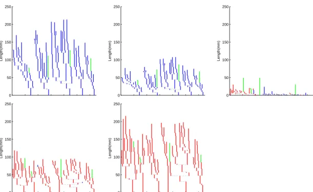
trimmed. (c) The result of this procedure is a cortical correspondence tree. . . 14 3.1 Example of a geodesic between artery trees showing five points along the
geodesic. Blue edges are only in the tree of the first subject, red only in the other subject and green are common to both (pendants are not included in this visualization). The drastic dip along the geodesic path is characteristic
for pairs of artery trees from this data set. . . 49 3.2 Ratio of number of interior edges versus maximal possible number of edges
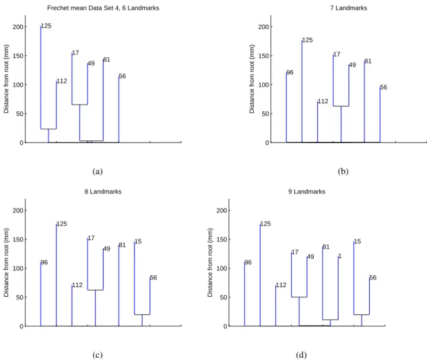
in Fr´echet means as a function of increasing the number of landmarks. . . 49 3.3 Tree views for the Frechet means for data sets having 6, 7, 8, and 9
landmarks. . . 50 3.4 Tree views for the Frechet means for data sets having 15, 16, 17, and 18
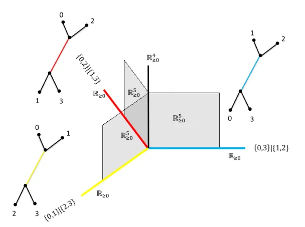
landmarks. . . 51 4.1 Depiction ofT3: three copies ofR5≥0,L1, L2, L3, each corresponding to
one of three possible tree topologies pasted together on a copy ofR4≥0,
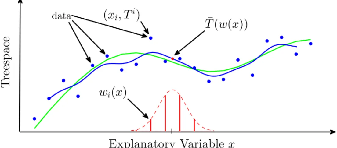
5.1 Schematic of Fr´echet kernel smoothing. Data are blue dots, a noisy sample from the green curve; the red dashed curve is a Gaussian kernel function and the vertical bars represent the relative weights of data points; red dot is kernel weighted mean atx,T¯(w(x)); and the blue curve is the kernel
smooth. . . 62 5.2 Kernel density estimate for distribution of subject ages. . . 64 5.3 Summaries from treesmooth family with bandwidthsh = 1,2,3,4,5,6
colored from blue to burgundy to red. Sum of lengths of interior edges
over age (top); and number of interior edges over age. . . 65 5.4 Scatter plots of number of interior edges and total length for smoothing
windowsh= 1,2,3,4,5,6years with the same colors as Fig. 5.3. We see a positive correlation between these variables indicating that their up and
down fluctuations across ages coincide. . . 66 5.5 Representative topology for treespace smooths with bandwidths h =
4,5,6. These bandwidths are large enough so the representative topology
for the treesmooth is equal to the topology of the overall Fr´echet mean. . . 67 5.6 Representative topologies for treesmooths for both bandwidthsh= 2,3.
The dotted edge in the left hand tree is the only edge which is not in the
LIST OF ABBREVIATIONS AND SYMBOLS
BHV Billera, Holmes, and Vogtman
LLN Law of Large Numbers
CHAPTER 1: INTRODUCTION 1.1 Dissertation Overview
Complex data objects arise in many areas of modern science including evolutionary biology, longitudinal studies, dynamics of gene expression and medical imaging. Object oriented data analysis (OODA) is the statistical analysis of datasets of complex objects. Theatoms of a statistical analysis are traditionally a number or a vector of numbers. In functional data analysis the atoms of interest are curves; for excellent treatment of functional data analysis see (Ramsay and Silverman, 2002, 2005). OODA progresses from functions to more complex objects such as images, two-dimensional or three-dimensional shapes, and combinatorial structures such as graphs or trees.
Data analysis of tree data objects, ortree oriented data analysis, is an exciting research area with interesting questions and challenging problems. This thesis focuses on tree oriented statistical methodologies, and algorithms for solving related mathematical optimization problems. The mathe-matical focus of this thesis is driven by the goal of analyzing a data set of images of human brain arteries collected by the CASILab at UNC-CH (Bullitt et al., 2008). From this perspective, this thesis is aimed at making contributions to morphology, the study of the form and structure of organisms.
A central question of tree oriented data analysis is “what are appropriate notions of mean and variance for a set of trees?” Typically, the mean of a dataset is specified as the sum of the observations divided by the number of observations. The mean of real numbers could also be specified as the solution to an optimization problem. An arithmetic mean is the real number that minimizes the sum of squared distances to data points. A more general notion of mean for metric spaces, called aFr´echet mean(a.k.a,barycenterorcenter of mass), is a point that minimizes the sum of squared distances to the data points. The Fr´echet mean is equivalent to the arithmetic mean in the case when data points are vectors. BHV treespaces have nice properties for statistics, including the existence of a unique shortest path between every pair of points, and the existence of a unique Fr´echet mean for a set of points. The focus of Ch. 2 is mathematical theory and methods for solving Fr´echet mean optimization problems defined for data sets on BHV treespace.
Prior to the research for this thesis, tube tracking algorithms were applied to a brain angiography dataset from the CASILab to reconstruct 3D models for the brain artery systems i.e. tubular 3D trees (Aylward and Bullitt, 2002). The main research advance for representing these trees as points in a BHV treespace was finding a morphologically interpretable fixed index set. The index set used in this research was determined by a technology in neuroimage analysis, called group-wise landmark based shape correspondence, which optimally places landmarks on the cortical surface of each member in a sample. This algorithm simultaneously optimizes a term which spreads landmarks out in each subject and a term which forces landmarks to similar positions for all subjects. More details about this representation of artery trees as points in a BHV treespace are explained in Sec. 1.3.
Results from analysis of this cortical landmark and brain artery data using Fr´echet means in BHV treespaces are presented in Ch. 3. In summary, these results show there is little similarity in the topological connections of brain arteries from the base of the brain to points where arteries are nearest to cortical landmarks, with the level of resolution available.
Fr´echet means in BHV treespaces exhibit an unusual stability property which is known as stickiness. Contrasting the typical behavior of sample means, where typically small changes in the
stratified spaces, e.g. data sampled from BHV treespaces, during the 2012 Object Oriented Data Analysis program at SAMSI. In this thesis, a new contribution to stickiness research is made, we characterize the limiting behavior of Fr´echet sample means on BHV treespaces as obeying asticky law of large numbers. This is the main result in Ch. 4.
Kernel smoothing is a flexible method for studying the relationships between variables. It is used in estimating probability densities and in regression. In Ch. 5, we present a novel method for kernel smoothing regression of tree-valued response against a real-valued predictive variable. This method is applied to the brain artery systems from the CASILab which will first be introducted in Sec. 1.3. The rest of this chapter is about phylogenetic trees and mapping brain artery trees to phylogenetic treespace.
1.2 Phylogenetic trees and BHV treespaces 1.2.1 Graphs and trees
A graphis a set of points, calledvertices (usevertex for a single point), and a set of lines connecting pairs of vertices, callededges. Atreeis a connected graph which has no cycles of edges and vertices. Thedegreeof a vertex is the number of edges connected to it. The vertices of a tree with degree one are called leaves, and the edges connected to them are calledpendants. Non-leaf vertices are calledinterior vertices. Edges which are not connected to leaves are calledinterior edges. Anedge weighted treeis a treeT together with a positive length|e|T associated with every edge e∈T. Contractingan edge means its length shrinks to zero thereby identifying its two endpoints to form a single vertex. A tree topologyT0that is created by contracting some edges in a treeT is called acontractionofT. Astar treeis a tree with only pendant edges.
1.2.2 Phylogenetic trees
Evolutionary histories or hierarchical relationships are often represented graphically as phyloge-netic trees. In biology, the evolutionary history of species or operational taxonomic units (OTU’s) is represented by a tree. Figure 1.1 is a very early graphical depiction of a phylogenetic tree from (Haeckel, 1866).
Alabeled treeis a treeTwithr+1leaves distinctly labeled using the index setI ={0,1, . . . , r}. Aphylogenetic treeis a labeled edge-weighted tree. The set of edges for a treeTis writtenET. Edge
einT is associated with asplit,Xe∪X¯einT. This is a partition ofIinto two disjoint sets of labels,
XeandX¯eon the two components ofT that result from deletingefromT, withXecontaining the
index0. Thetopology of a phylogenetic treeis the underlying graph and pendant labels separated from the edge lengths. The topology of a phylogenetic tree is uniquely represented by the set of splits associated with its edges. Formally, two splitsXe∪X¯eandXf ∪X¯f arecompatibleif and only if
Xe⊂Xf andX¯f ⊂X¯e, orXf ⊂XeandX¯e⊂X¯f. Compatibility can be interpreted in terms of
subtrees: the subtree with leaves in bijection withX¯econtains the subtree with leaves in bijection
withX¯f, or vice versa. If every pair of splits in a set of splits is compatible then that set is said to be
a compatible set. Each distinct set of compatible splits is equivalent to a unique phylogenetic tree topology. A maximal tree topology is one in which no additional interior edges can be introduced i.e. |ET|= 2r−1, or equivalently every interior vertex has degree 3.
1.2.3 Construction of BHV Treespaces
A BHV treespace,Tris a geometric space in which each point represents a phylogenetic tree
having leaves in bijection with a fixed label set{0,1,2, . . . , r}.
Anon-negative orthantis a copy of the subset ofn-dimensional Euclidean space defined by making each coordinate non-negative,Rn≥0. Here, only non-negative orthants are used, so we use orthant to mean non-negative orthant. Anopen orthantis the set of positive points in an orthant. Phylogenetic treespace is a union of many orthants, each corresponding to a distinct tree topology, wherein the coordinates of a point are interpreted as the lengths of edges. For a given set of compatible edgesE, the associated orthant is denotedO(E), and for a given treeT, the orthant in treespace containing that point is denotedO(T). Trees inTrhave at mostr−2interior edges. Each orthant
of dimensionr−2corresponds to a combination ofr−2compatible edges. Orthants are glued together along common faces. The shared faces of facets withkpositive coordinates are called the k-dimensional faces of treespace.
orthants are glued together along common axes. Views of the two main features ofT4 are displayed in Figure 1.2. See Figure 1.3 for a visualization of the split-split compatibility graph ofT41.
Each clique in the split-split compatibility graph represents a compatible combination of splits, or equivalently the topology of a phylogenetic tree. A graph iscompleteif there is an edge between every pair of vertices. In a graph, acliqueis a complete subgraph. Each full phylogenetic tree is a maximal clique in the split-split compatibility graph because a clique represents a set of mutually compatible splits. The split-split compatibility graph ofT4 has fifteen maximal cliques, each of which is represented an edge in the graph. The split-split compatibility graph ofT4determines how the orthants ofT4are glued.
1.3 Brain artery data
The brain artery trees used in this study were reconstructed from a data set of Magenetic Resonance (MR) brain images collected by the CASILab at the University of North Carolina at Chapel Hill. This data set is publicly available and hosted at the MIDAG website (Bullitt et al., 2008). The database has images for various magnetic resonance modalities, including T1, T2, Magenetic Resonance Angiography (MRA), and Diffusion Tensor Imaging (DTI). The study enrolled 109 apparently healthy subjects. Each image is tagged with subject features of age, sex, handedness and self-identified race. The MRA was aquired at 0.5 x 0.5 x 0.8 mm3 accuracy.
Arteries branch out mostly as a tree from the heart and deliver blood to the entire body. In particular arteries transport oxygen and nutrient-rich blood to the brain. Magnetic Resonance Angiography (MRA) is a technique in medical imaging to visualize arteries. MRA uses the fact that blood flowing in the arteries has a distinct magnetic signature. Full 3D image acquisition is achieved by combining cross sectional 2D images. See Figures 1.4 and 1.5 below for an MRA slice and an artery reconstruction for the same subject. A limiting factor is that MRA has a resolution threshold and consequently there are arteries that are too small for detection. MRA detects only arteries which feed blood rich with oxygen and nutrients to the body, and not veins which carry depleted blood back to the heart.
The arteries visible in MRA are generally naturally described as a tree. In most regions of the body and at the level of resolution possible, arteries branch like a tree without any loops. A major
1
part of this research has been opening up the possibility of using the space of phylogenetic trees as a mathematical basis for developing statistical methods for the study of artery trees. Phylogenetic trees have a common leaf set. However artery trees do not. A common leaf set is artificially introduced by determining points on the cortical surface that correspond across different people. The next section describes the details of representing brain artery systems as points in BHV treespace.
1.4 Mapping Brain Artery Systems to BHV treespace
Figure 1.6(a) gives a detailed view of artery centerlines. Each tree consists of branch segments, and each branch segment consists of a sequence of spheres fit to the bright regions in the MRA image. The sphere centers are 3D points on the center line of the artery, and the radius approximates the arterial thickness. A method for visualizing the structure of large trees was used to detect any remaining discrepancies (Aydin et al., 2009b).
1.4.1 Correspondence
1.5 Other approaches to tree oriented data analysis
The branching structures of blood arteries and pulmonary airways are naturally modeled as trees. There is a large scope for progress in statistics for a population of trees. Currently, at the time that this dissertation is being written, research in tree oriented data analysis includes four major directions: combinatorial trees, Dyck paths, treeshapes and phylogenetic trees.
A seminal papaer in thecombinatorial tree approachto studying populations of anatomical trees laid foundations by proposing a metric, several notions of center, variation, and a method of principal components (Wang and Marron, 2007). Later fast PCA algorithms for combinatorial trees were developed (Aydin et al., 2009a). The most recent innovation for combinatorial tree is smoothing method for nonparametric regression with combinatorial tree structures as response variables against a univariate Euclidean predictor (Wang et al., 2011) .
Another approach uses a Dyck path mapping of trees to curves (Harris, 1952). A Dyck path for a tree is produced by recording the distance on the tree to the root vertex during a depth first left to right traversal. Representing trees as Dyck paths opens up the possibility to use methods such as functional PCA (Shen et al., 2012).
Thetreeshape approachis an area of active research. A tree-shape is a graph theoretic tree with a real matrix of fixed dimensions associated with each edge of the tree. Tree-shapes and statistics for tree-shapes were introduced in (Feragen et al., 2012). This approach allows very general descriptions of trees and thus allows for much richer representations of anatomical trees such as lungs or arteries than the above approaches. The generality of this approach comes with the cost of a very complicated sample space. A related approach, unlabled-trees, is a special case of treeshape, where the edge attributes are restricted to be non-negative numbers.
1.5.1 BHV treespace geodesics
We now give an explicit description of geodesics in treespace.
LetX ∈ Trbe a variable point and letT ∈ Trbe a fixed point. LetΓXT ={γ(λ)|0≤λ≤1}
be the geodesic path fromXtoT. LetCbe the set of edges which are compatible in both trees, that is the union of the largest subset ofEX which is compatible with every edge inT and the largest
The following notation for the Euclidean norm of the lengths of a set of edgesAin a treeT will be used frequently,
||A||T = s
X e∈A
|e|2
T (1.1)
or without the subscript when it is clear to which tree the lengths are from.
A support sequence is a pair of disjoint partitions,A1∪. . .∪Ak=EX\CandB1∪. . .∪Bk=
ET \C.
Theorem 1.5.1. (Owen and Provan, 2009) A support sequence(A,B) = (A1, B1), . . . ,(Ak, Bk)
corresponds to a geodesic if and only if it satisfies the following three properties:
(P1) For eachi > j,AiandBj are compatible
(P2) kA1k kB1k ≤
kA2k
kB2k ≤. . .≤ kAkk kBkk
(P3) For each support pair(Ai, Bi), there is no nontrivial partitionC1∪C2ofAi, and partition
D1∪D2ofBi, such thatC2is compatible withD1and kkDC1k1k < kkCD22kk
The geodesic betweenXandT can be represented inTnwith legs
Γl= h
γ(λ) : 1−λλ ≤ kA1k kB1k
i
, l= 0
h
γ(λ) : kAik kBik ≤
λ
1−λ ≤
kAi+1k kBi+1k
i
, l= 1, . . . , k−1,
h
γ(λ) : 1−λλ ≥ kAkk kBkk
i
, l=k
The points on each legΓlare associated with treeTlhaving edge set
El = B1∪. . .∪Bl∪Al+1∪. . .∪Ak∪C
Lengths of edges inγ(λ)are
|e|γ(λ)=
(1−λ)kAjk−λkBjk
kAjk |e|X e∈Aj
λkBjk−(1−λ)kAjk
kBjk |e|T e∈Bj
The length ofΓis
d(X, T) = w w w w
(kA1k+kB1k, . . . ,kAkk+kBkk,|eC|X − |eC|T)
w w w w
(1.2)
0,1
|{2
,3
,4
}
0,1,2 |{3,4}
0
1
2
3 4 0
1
2 3
4 0
1
2
3
4
(a) An open half book with three pages. In this diagram thepagesof the book are three copies of
R2≥0and thespineis a copy ofR≥0. The spine is labeled with the split{0,1}|{2,3,4}. Each page
has the spine as one axis and the other axis is labeled with a split compatible with{0,1}|{2,3,4}. InT4every one of the ten splits of{0,1,2,3,4}is the label for the spine of the open half book.
{0,
1}|{2,
3,
4}
0
1
2
3
4
0
1 2
3
4
0
1 2
3 4
(b) A five-cycle. Afive-cycleis five copies ofR2≥0glued together along commonly labeled axes
and at their origins.
{0,1,2}|{3,4} {0,1,3}|{2,4}
{1,3}|{0,2,4}
{0,1}|{2,3,4}
{0,1,4}|{2,3}
{0,2}|{1,3,4}
{0,3}|{1,2,4} {1,2}|{0,3,4}
{0,4}|{1,2,3}
{1,4}|{0,2,3}
Figure 1.3: Split-split compatibility graph ofT4. Each split has a node. Two splits are compatible if they are joined by an arc. This shows the overall connectivity of T4, all possible splits for {0,1,2,3,4}, and all possible topologies for 4-trees. Each vertex and the three edges emanating from it in the graph corresponds to a copy of an open book like in Figure 1.2(a). Each five-cycle in the graph is a copy of a five-cycle depicted in Figure 1.2(b)
(a) (b)
(c)
CHAPTER 2: Methods for Fr´echet Means in Phylogenetic Treespace 2.1 Introduction
The central research problem of this chapter is efficient computation of the Fr´echet mean of a discrete sample of points in BHV treespaces. The novel algorithmic system designed in this research project improves upon the current solution methodologies in (Miller et al., 2012) (Ba˘c`ak, 2012). These methods are applied to the sample of brain artery trees introduced in Chapter 1.
The contents of this Chapter are organized as follows: In Sec. 2.1.1 we define the Fr´echet mean in BHV treespace, and give an overview discussion of the Fr´echet optimization problem. In Sec. 2.2 we present global methods for optimizing the Fr´echet function i.e. methods which can move from one orthant of treespace to another. In Sec. 2.3 we describe how the combinatorics of treespace geodesics lead to polyhedral subdivision of treespace into regions where the Fr´echet function has a fixed algebraic form. The focus of Sec. 2.4 is differential properties of the Fr´echet function. In Sec. 2.5.1, a method finding the minimizer of the Fr´echet function in a fixed orthant of treespace is presented. Application of these method to brain artery systems is the focus of Ch. 3.
2.1.1 Fr´echet means in BHV treespace
For a given data set of n phylogenetic trees T1, T2, . . . , Tn in Tr, the Fr´echet function is the sum of squares of geodesic distances from the data trees to a variable tree X. A geodesic γ : [0,1]→ Tris the shortest path between its endpoints. The geodesic fromXtoTiis characterized by a geodesic support,(Ai,Bi) = (Ai
1, B1i), . . . ,(Aiki, Bkii)
(Thm. 1.5.1). Given the geodesic supports(A1,B1), . . . ,(An,Bn)the Fr´echet function is
F(X) = n X
i=1
d(X, Ti)2= n X i=1
ki
X l=1
(kxAi lk+kB
i lk)2+
X e∈Ci
(|e|T − |e|Ti)2
. (2.1)
The objective is to solve the Fr´echet optimization problem
min X∈Tr
Elementary Fr´echet function properties:
• The Fr´echet function is continuous because the geodesic distancesd(X, Ti)are continuous
(Owen and Provan, 2009; Miller et al., 2012).
• The Fr´echet functionF(X)is strictly convex (Sturm, 2003), that isF ◦γ : [0,1]→ Ris
(strictly) convex for every geodesicγ(λ)inTr.
As a consequence of these properties we have the following result. Lemma 2.1.1. The Fr´echet mean exists and is unique.
Proof. A strictly convex function either has a unique minimizer or can be made arbitrarily low. Assuming that the data points are finite, then a minimizer of the Fr´echet function must also be finite. Therefore the Fr´echet function has a unique minimizer.
The Fr´echet meanT¯is the unique minimizer of the Fr´echet function.
2.1.1.1 Problem Discussion
The Fr´echet optimization problem, in BHV treespace, requires both selecting the minimizing tree topology and specifying its edge lengths. Tree topologies are discrete and so the problem of selecting the minimizing tree topology is a combinatorial optimization problem; however it is possible to make search strategies which take advantage of the continuity of BHV treespace to find the correct tree topology. It is natural to consider this problem in two modes of search: global, i.e. strategies which change the topology and edge lengths; and local, i.e. strategies which only adjust edge lengths. One motivation to consider global search and local search separately is that the local optimization problem is convex optimization constrained to a Euclidean orthant.
a contraction. However, the list of tree topologies which have a particular treeXas a contraction can be quite large. For example, ifXis a star tree thenXis a contraction of any tree i.e.X is a contraction of(2r−3)!!maximal phylogenetic tree topologies.
Local optimality conditions for non-differentiable functions are based on the rate of change of the objective function along directions issuing from a point. Since the neighborhood of a pointXcontains all trees which haveX as a contraction, verifying thatX is optimal requires demonstrating that any tree which containsXas a contraction has a larger Fr´echet function value. For example, when Xis a star tree,N(X)contains every tree with the same pendants asX, and having infinitesimal interior edge lengths. In this sense finding a descent direction can be essentially as hard as finding the topology of the Fr´echet mean itself.
Proximal point algorithms, a broad class of algorithms, are globally convergent not only for the Fr´echet optimization problem, but are globally convergent for any well defined lower-semicontinuous convex optimization problem on a non-positively curved metric space (Ba˘c`ak, 2012). This class of algorithms has nice theoretical properties, and certain implementations of proximal point algorithms are practical for the Fr´echet optimization problem on non-positively curved orthant spaces.
Proximal point algorithms are applicable to optimization problems on metric spaces. The general problem is minimizing a functionf on a metric spaceM with distance functiond:M×M →R. A proximal point algorithm solves a sequence of penalized optimization problems of the form
Pk(f) : min xk f(x
k) +α
kd2(xk−1, xk) (2.3)
where αk influences the proximity of a solution to the point xk−1. Some good references for
proximal point algorithms are (Baˇc´ak, 2012; Bertsekas, 2011; Li et al., 2009; Rockafellar, 1976). Implementing a generic proximal point algorithm to minimize the Fr´echet function on treespace does not seem advantageous. In particular, given a non-optimal pointX0 finding a pointXsuch that F(X)< F(X0)is not made any easier by penalizing the objective functionF(X) +αd2(X0, X). Penalizing the objective function withαd(X0)does not provide any additional structure for checking the neighborhood,N(X0), ofX0for a descent direction.
a sum of functions,f =f1+. . .+fm, a split proximal point algorithm alternates among penalized optimization problems for each function. Let {1,2, . . . , m} index the functions f1, . . . , fm. A generic split proximal point algorithm is: choose some sequencei1, i2, . . .where each term in the sequence is an element of{1,2, . . . , m}and sequentially solve the split proximal point optimization problem:
Pk(fik) : min xk f(x
k) +α
kd2(xk−1, xk) (2.4)
Different versions of split proximal point algorithms are based on the choice of the sequencei1, i2, . . . and the choice of the sequence{αk}. Naturally, a split proximal point procedure can be applied to
the Fr´echet optimization problem by separating the Fr´echet function into a sum of squared distance functions,F(X) =d2(X, T1) +. . .+d2(X, Tn). For the Fr´echet function the split proximal point optimization problem is
Pk(d2(Xk, Tik)) : min
xk d
2(Xk, Tik) +α
kd2(Xk−1, Xk) (2.5)
For the Fr´echet mean optimization problem on a geodesic non-positively curved space, the solution to a split proximal point optimization problem can be obtained easily in terms of geodesics. The solution toPk(d2(Xk, Tik))must be on the geodesic betweenXk−1 andTik. The termd2(Xk, Tik)is the
squared distance from the variable point toTikand the termd2(xk−1, xk)is the squared distance from
the search point toXk−1. Given any point, there is at least one point on the geodesic betweenXk−1 andTik for which the value of both terms is at least as small. SinceXkmust be on this geodesic, the
distance fromXktoXk−1and the distance formXktoTik can be parameterized in terms of the
proportiont: 0≤t≤1along the geodesic fromXk−1toTik:d(Xk, Tik) = (1−t)d(Xk−1, Tik)
andd(Xk, Xk−1) =td(Xk−1, Tik). Parameterizingd2(Xk, Tik) +α
kd2(Xk−1, Xk)in terms of
tmakes Pk(d2(Xk, Tik))into a problem of minimizing a quadratic function in t. The optimal
The overall strategy for minimizing the Fr´echet function will be to use a split proximal point algorithm for global search and switch to a local search procedure. The motivation for switching to a local search procedure is that the if local search is initialized close to the optimal solution then faster convergence can be achieved. The local optimization problem is minimizing the Fr´echet function in a fixed orthantO. One feature of the local optimization problem is that the Fr´echet function is a piecewiseC∞function whose algebraic form depends on the geodesic distance fromX to the data trees. But, the Fr´echet function is onlyC1 whenXis restricted to the interior of a maximal dimension orthant. Analysis of differential properties of the Fr´echet function is presented in Sec. 2.4.
InTr, the Owen-Provan algorithm for the geodesicΓ(X, Ti)has complexityO(r4), and with ndata points the total complexity of finding the algebraic form ofF(X)would beO(nr4). New algorithms for dynamically updating the algebraic form ofF(X)asXvaries are presented in Section 2.6. Such algorithms will be especially useful in updating the objective function after small changes are made in the edge lengths ofX; in particular these methods help accelerate local search algorithms.
Here is a high-level outline of the algorithmic system for solving the Fr´echet mean optimization problem developed in this chapter:
Treespace Fr´echet mean algorithm
input:T1, T2, . . . , Tn, X0∈ Tr, >0,δ >0,a >0,0< c <1,{αk},K ∈N
F0= inf;F1=F(X0)
whileF1−F0 > a
SPPA forK steps (Sec. 2.2) c=1;
whilec≤K
Xk=argminX
d2(X, Tik) +α
kd2(Xk−1, X)
endwhile
whileapproximate optimality conditions (2.5) are not satisfied compute a descent directionP (Sec. 2.5.1.1)
find a step-length,α, satisfying decrease condition (Sec. 2.5.1.2) letXk+1 =Xk+αP
endwhile endwhile
The following sections discuss implementation details and present theoretical analysis pertaining to certain aspects of the problem. The next section presents specific global search procedures, both of which are versions of split proximal point algorithms. The remaining sections focus on aspects of the local search problem.
2.2 Global search methods
Proximal point algorithms as applied to the Fr´echet optimization problem have been studied in (Ba˘c`ak, 2012) and (Sturm, 2003). The former views the Fr´echet mean problem from the paradigm of convex optimization while the later studies Fr´echet means in the context of stochastic analysis in metric spaces of non-positive curvature. In this Chapter two global search algorithms are discussed, theInductive Mean Algorithm, which is stochastic, and theCyclic Split Proximal Point Algorithm, which is deterministic. Both of these are versions of split proximal point algorithms.
2.2.1 Inductive means
TheInductive Mean Algorithmis a method for calculating the Fr´echet Mean based on (Sturm, 2003, Thm. 4.7). This algorithm was developed independently in (Ba˘c`ak, 2012) and (Miller et al., 2012) and has been called Sturm’s algorithm, named after the K. T. Sturm who is attributed with its discovery in proving that inductive means converge to the Fr´echet mean in the more general context of probability distributions on non-positively curved metric spaces.
Consider a sequence(Yi)i∈Nof independent identically distributed random observations from
the uniform distribution on{T1, T2, . . . , Tn}. Define a new sequence of points(S
k)k∈NinTrby
induction onkas follows:
S1:=Y1,
and
Sk:=
1− 1 k
Sk−1+
1
kYk,
where the right hand side denotes the point k1 fraction of the distance along the geodesic fromSk−1 toYk. The pointSkis called theinductive mean valueofY1, . . . , Yk. The expected squared distance
2.2.2 Cyclic Split Proximal Point Algorithm
Choose a permutation,(p0, p1, . . . , pn−1), of{1,2, . . . , n}. Define a new sequence of points
(Rk)k∈NinTrby induction onkas follows:
R1:=Yp1,
and
Rk:=
1−1 k
Rk−1+
1
kYp(kmodn).
The sequence{Rk}converges toT¯askapproaches infinity (Ba˘c`ak, 2012). 2.3 Vistal cells and squared treespace
The value of the Fr´echet function atXdepends on the geodesics fromXto each of the data trees. The goal in this section is to describe how treespace can be subdivided into regions where the combinatorial form of geodesics fromXto the data trees are all fixed. Descriptions of such regions will be used in analyzing the differential properties of the Fr´echet function.
Analysis of the Fr´echet function starts at the level of a geodesic from avariable treeXto a fixed source treeT. Given a fixed treeT, a vistal cell is a regionV of treespace where the form of the geodesic from any treeXinVtoT is constant. The description of geodesics in Section 1.5.1 is now built upon further to study how the combinatorics of geodesic supports forΓ(X, T)can vary asX varies.
Definition 2.3.1. (Miller et al., 2012, Def. 3.3) LetT be a treeTr. LetObe a maximal orthant containingT. Theprevistal facet,V(T,O;A,B), is the set of variable trees,X∈ O, for which the geodesic joiningXtoThas support(A,B)satisfying(P2)and(P3)with strict inequalities.
The description of the previstal facetV(T,O;A,B)becomes linear after a simple change of variables. Letxedenote the coordinate inTrindexed by edgee.
Definition 2.3.2. (Miller et al., 2012, Def. 3.4) Thesquaring mapTr → Tracts onx∈Tr ⊂RE+ by squaring coordinates:
Denote byT2
r the image of this map, and letξe=x2edenote the coordinate indexed bye∈E.
The image of an orthant in Tr is then the equivalent orthant inTr2, and the image of a previstal
facetV(T,O;A,B)inT2
r is avistal facetdenoted byV2(T,O;A,B). With this change of variables,
kSk=P e∈Sξe.
The squaring map induces on the Fr´echet functionF a corresponding pullback function
F2(ξ) =F(pξ), where(pξ)e= p
ξe.
Since the Fr´echet functionF(X)has a unique minimizerF2(ξ)must also have a unique minimizer. Proposition 2.3.3. (Miller et al., 2012, Prop. 3.5) The vistal facet V2(T,O;A,B) is a convex polyhedral cone inT2
r defined by the following inequalities onξ∈Rr−2.
(O) ξ∈ O; that is,ξe≥0for alle∈E, andξe= 0fore /∈E, whereO=Rr≥−02.
(P2) kBi+1k2
X e∈Ai
ξe≤ kBik2 X e∈Ai+1
ξefor alli= 1, . . . , k−1.
(P3) kBi\Jk X e∈Ai\I
ξe≥ kJk X
e∈I
ξefor alli= 1, . . . , kand subsetsI ⊂Ai,J ⊂Bisuch that
I∪Jis compatible.
Proposition 2.3.4. (Miller et al., 2012, Prop. 3.6) The vistal facets are of dimension2r−1, have pairwise disjoint interiors, and coverT2
r . A pointξ ∈ Tr2lies interior to a vistal facetV2(T,O;A,B)
if and only if the inequalities in (O), (P2), and (P3) are strict.
Points which are not on the interior of vistal facets are invistal cells, the faces of vistal facets. A pointξis on a vistal facet precisely when some of the inequalities in (O), (P2) or (P3) are satisfied at equality. In such a situation, there is more than one valid support for the geodesic fromT to the pre-imageXofξ.
A system of equations defining a vistal cell can be formed by combining the systems of equations from adjacent vistal facets and forcing appropriate constraints to equality. A canonical description of vistal cells is given in (Miller et al., 2012, Sec. 3.2.5).
LetT1, . . . , Tnbe a set of points inTr. A regionV in squared treespace where the geodesics ΓXT1, . . . ,ΓXTncan be represented by a fixed set of supports is called avistal cell. A
inTr,pre-multi-vistal cells, are regions where the Fr´echet function can be represented with a fixed algebraic form.
The systems of equations defining pre-vistal facets and pre-vistal cells are quadratic cones with cone points at the origin of treespace. In squared treespace, the vistal facets and vistal cells are polyhedral cones. Multi-vistal facets are also polyhedral cones with cones points at the origin of treespace, because they are intersections of polyhedral cones with cone points at the origin of treespace. This nice geometric structure is useful both in determining when a search point is on the boundary of a vistal cell, and thus when the objective function has multiple forms, and for dynamically updating the objective function during line searches, as described in Sec. 2.6.
2.4 Differential analysis of the Fr´echet function in treespace
Analysis of howF(X)changes with respect toX provides useful insights for designing fast optimization algorithms. This analysis is aimed at providing summaries for how the value ofF(X)
changes with respect toX. These results also play an important role in Ch. 4, which focuses on stickiness of Fr´echet means in treespace.
LetXandY be points inTrsuch thatXandY share a multi-vistal facet. If this is the case, then
either (i)XandY have the same topology, (ii)X is a contraction ofY or (iii)Y is a contraction ofX. Assume that if the topologies of treesXandY differ thenX is a contraction ofY, that is O(X)⊆ O(Y). LetΓ(X, Y;α)be the parameterized geodesic fromXtoY with0≤α≤1.
Definition 2.4.1. Thedirectional derivative fromXtoY is
F0(X, Y) = lim α→0
F(Γ(X, Y;α))−F(X)
α (2.6)
The main results of this section are summarized as follows: Cor. 2.4.3 gives the value of the directional derivative whenO(X) =O(Y)and Thm. 2.4.7 gives the value of the directional derivative whenO(X) ⊆ O(Y), when assumingY is contained on the interior of a multi-vistal facet. In Lem. 2.4.8 we show that when whenY is on a multi-vistal face the value of the directional derivative can be expressed equivalently using any of the representations for the geodesics from T1, . . . , TntoY. In Lem. 2.4.9 and Lem. 2.4.11 we show that the directional derivative is continuous and convex with respect toY onTr. Thm. 2.4.17 states that the value of the directional derivative can
edges inX, and a contribution from the change inF(X)resulting in increasing the lengths of edges from zero.
When bothXandY are in the relative interior of the same maximal orthant of treespace, where the gradient atX is well defined inO(Y), the directional derivative can be expressed in terms of the gradient atXinsideO(Y). However whenO(X)$O(Y), the gradient atXmight not be well
defined inO(Y). Analysis of the directional derivative in the later situation, which is one of the main focuses of this section, is important because it facilitates concise specification of optimality conditions and an efficient algorithm for verifying that a point on a lower dimensional face of an orthantOis the minimizer of the Fr´echet function withinO.
Theorem 2.4.2. (Miller et al., 2012)[Thm. 2.2] The gradient ofF is well defined on the interior of every maximal orthantO.
Idea of proof. The Fr´echet function is smooth in each multi-vistal facet, and it can be shown that the gradient function has the same value in every multi-vistal facet containingXin the interior ofO. Therefore the gradient is well -defined on the interior ofO.
Corollary 2.4.3. When O(X) = O(Y) the value of directional derivative fromX toY can be expressed in terms of the gradient atX, and the differences in edge lengthspe=|e|Y − |e|X, as
F0(X, Y) = X e∈EX
pe[∇F(X)]e (2.7)
Proof. Expression of a directional derivative of a smooth function in terms of its gradient is a standard technique in calculus.
The gradient may not be well defined on a lower-dimensional orthant of treespace. For a point on a lower dimensional orthant of treespace, a well defined analogue to the gradient is therestricted gradient.
Definition 2.4.4. Let(Ai1, B1i), . . . ,(Aiki, Bkii)be a support sequence for the geodesic fromXto
O(X)⊆ O(Y)andY −Xparallel to the axes ofO(X). If|e|X >0then
[∇F(X)]e= lim
∆e→0
F(X+ ∆e)−F(X)
∆e (2.8)
= n X i=1 |e|X
1 +||Bli|| ||Ai
l||
ife∈Ail
(|e|X − |e|Ti) ife∈Ci
(2.9)
and if|e|X = 0then[∇F(X)]e= 0.
WhenXis on the interior of a maximal orthant of treespace then the restricted gradient is the same as the gradient. Note that in the case whenAil={e},|e|X1 +||Bil||
||Ai l||
=|e|X +kBi lk.
Second order derivatives will be used in calculating Newton directions in Sec. 2.5.
Definition 2.4.5. LetXbe a point in the interior of a multi-vistal cell relative to an orthantOof treespace. The restricted Hessian onOis the matrix of second order partial derivatives with entries having the following values:
∇2F(X) ef = 2
r X i=1
1 +kB
i lk kAi
lk
− kBlik kAi
lk3
x2e ife=f,e∈Ail,|Ai l|>1 1 ife=f,e∈Ail,Ail={e}
1 ife=f e∈Ci
−kBlik kAi
lk3
xexf ife6=f e, f ∈Ail
0 otherwise
(2.10)
If either|e|X = 0or|f|X = 0then
∇2F(X) ef = 0.
Theorem 2.4.6. The value of the restricted gradient at a pointX can be expressed equivalently using the algebraic form of the Fr´echet function from any of the multi-vistal facets containingX.
Proof. The restricted gradient has the same value using any of the valid support sequences defined by vistal cells on the relative interior ofO. Here we verify that atXthe gradient ofd2(X, Ti)is the same for every valid support and signature. The gradient ofd2(X, Ti)for the support(A,B)is given as follows. Let the variable length of edgeeinXbe written asxe.
∂d2(X, Ti)
∂xe =
21 +||Bl|| ||Al||
xe ife∈Ail 2 xe− |e|iT
ife∈Ci
The geodesicΓhas a unique support(A,B)satisfying
kA1k kB1k <
kA2k
kB2k < . . . < kAkk
kBkk. (2.12)
From (Miller et al., 2012), any other support(A0,B0)forΓmust have a signatureS0in(P3)with some equality subsequences. Suppose thatA0jandBj0 are in some equality subsequence satisfying
(P2)withB0jcontaining the edgee. Then for the support pairAiandBisuch thatBicontainse, it
must hold that kA 0
ik kBi0k =
kAjk
kBjk. Now we can see that
1 +||B
0
j|| ||A0j||
xe=
1 +||Bi|| ||Ai||
xe, and that the
gradient ofd2(X, Ti)is the same on every multi-vistal facet containingXon the relative interior of O.
Now we extend the results for directional derivatives to the situation whenO(X)⊂ O(Y). Theorem 2.4.7. Suppose thatY lies in the interior of multi-vistal facetVY, andXis some point in
VY. Let(Ai1, B1i), . . . ,(Ain, Bni)be the support pairs for the geodesic fromY toTiand letCibe
the set of edges inY which are common inTi. LetEX be the set of edges with positive lengths in
X. LetP be the vector with componentspe=|e|Y − |e|X so thatΓ(X, Y;α) =X+αP, and let
Zα := Γ(X, Y;α). Then the value of directional derivative fromXtoY is
F0(X, Y) = X e∈EX
pe[∇F(X)]e+ 2 n X i=1 X l:kAi
lkX=0
kAi
lkPkBlikT
− X
e∈Ci\E X
pe|e|Ti
.
Proof. LetZbe a point on the geodesic segment betweenXandY. The length of edgeeinZbe |e|Z =|e|X +αpe. The Fr´echet function is the sum of squared distances from a variable point to
each of the data pointsT1, . . . , Tn, so the directional derivative of the Fr´echet function is the sum over the indexes of the data points of the directional derivatives of the square distances.
F0(X, Y) = lim α→0
F(Zα)−F(X)
α (2.13)
= lim α→0
Pn
i=1d2(Zα, Ti)−Pni=1d2(X, Ti)
α (2.14) = n X i=1 lim α→0
d2(Zα, Ti)−d2(X, Ti)
α
For a set of edgesA, letkAkX =pP
e∈A|e|X. If an edgeehas zero length in a tree,X, or is
compatible withXbut not present then take|e|X to be0. The squared distance fromZαtoTican
be expressed as
d2(Zα, Ti) = ki
X l=1
(kAilkZα+kB
i lk)2+
X e∈Ci
(|e|Zα− |e|Ti)2. (2.16)
The squared distance has three types of terms: a term representing the contribution from common edges, terms for support pairs withkAi
lkX >0, and terms for support pairs withkAilkX = 0. In the
first two cases the gradient is well-defined, and taking the inner-product of the directional vector and the gradient will yield their contributions to the directional derivative. In the third case the gradient is undefined, and its value will be obtained by analyzing the limit directly as follows.
lim α→0
Pki
l=1(kAilkZα +kB
i lk)2−
Pki
l=1(kAilkX+kBlik)2
α
!
. (2.17)
Bringing out the sum and canceling in the numerators yields,
ki
X l=1
lim α→0
kAi
lk2Z− kAilk2X + 2kBlik kAilkZ− kAilkX
α . (2.18)
The limit of the fraction can be split into the sum of two limits,
lim α→0
kAi
lk2Z− kAilk2X + 2kBlik kAilkZ− kAilkX
α (2.19)
= lim α→0
kAi
lk2Z− kAilk2X
α + limα→0
2kBi
lk kAilkZ− kAilkX
α . (2.20)
If every edge inAilhas length zero inX, and thuskAi
lkX = 0, the expression the limit on the left is
zero and the limit on the right simplifies to
The partial derivative of the squared distance fromXtoTiwith respect to the length of edgee, that is the component for edgeein the restricted gradient vector, is
[∇d2(X, Ti)]e= |e|X
1 +||Bil|| ||Ai
l||
ife∈Ai l
(|e|X − |e|Ti) ife∈Ci.
(2.22)
The directional derivative of the squared distance simplifies to
lim α→0
d2(Z, Ti)−d2(X, Ti)
α (2.23)
= X
e∈EX
pe[∇d2(X, Ti)]e+ 2 X l:kAi
lkX=0
kBlik s
X e∈Ai l
p2
e
−2
X e∈Ci\E
X
pe|e|Ti. (2.24)
Summing the directional derivatives of the squared distances overT1, . . . , Tnyields the expression for the value of the directional derivative in the theorem.
We now extend the results to the situation whereY is allowed to be on a vistal face. In this situation there can be multiple valid support sequences for the geodesics fromY toT1, . . . , Tn. Lemma 2.4.8. Suppose thatXandY are in the same multi-vistal facet,V, and thatY is on a face of Von the interior of an orthant. The value of the directional derivative can be expressed equivalently
using any valid support sequences for the geodesics fromY toT1, . . . , Tn.
(Ai1, Bi1), . . . ,(C1, D1),(C2, D2), . . . ,(Aim, Bmi ); and
kC1k kD1k =
kC2k kD2k =
kAi lk kBi
lk
. Rescaling the lengths of edges inAildoes not change the form of the geodesic for smallαandl≤k. Parameterizing the lengths of edges in terms ofαand cancelingαyields
qP
e∈C1p2e kD1k =
qP
e∈C2p2e kD2k =
qP
e∈Ai l
p2 e
kBi lk
. That fact, and the fact thatC1∪C2partitionAilandD1∪D2partitionBliimplies thatkD1kqP
e∈C1p
2 2+ kD2kqP
e∈C2p
2
e =kBlik
qP
e∈Ai lp
2
e. Thus the directional derivative is continuous across vistal
facet boundaries from (P2) and (P3) constraints.
Now we extend the results for directional derivatives to directions issuing fromXto pointsY in a small enough radius such thatO(X)⊆ O(Y)andXandY share a multi-vistal facet.
Lemma 2.4.9. The directional derivative,F0(X, Y), is a continuous function ofY over the set ofY such thatO(X)⊆ O(Y)andXandY share a vistal facet.
Proof. The directional derivative is a continuous function at the faces of orthants because when an edge length|e|Y increases from zero its contribution toF0(X, Y)is a continuous function which
starts at the value zero. Thus, when the topology ofY changesF0(X, Y)changes continuously as a function of the edge lengths.
The following lemma is used in the proof of Lem. 2.4.11.
Lemma 2.4.10. LetY0andY1be a points inTrsuch thatO(X)⊆ O(Y0)andO(X)⊆ O(Y1).
LetYt= Γ(Y0, Y1;t)be the point which is proportiontalong the geodesic fromY0toY1. The point which isαproportion along the geodesic fromXtoYtistproportion along the geodesic between the pointΓX,Y0(α)and the pointΓX,Y1(α); that is,Γ(X, Yt;α) = Γ(Γ(X, Y0;α),Γ(X, Y1;α);t).
Proof. LetY0(α) = ΓXY0(α)and letY1(α) = ΓXY1(α). LetC=EY0(α)∩EY1(α). By definition
EX ⊆C. The length ofeinY0(α)is
|e|Y0(α)=
|e|X +α|e|Y0 ife∈C
α|e|Y0 ife∈EY0\C
(2.25)
and the length ofeinY1(α)is
|e|Y1(α)=
|e|X +α|e|Y1 ife∈C
α|e|Y1 ife∈EY1 \C.
A geodesic support sequence which is valid for the geodesic betweenY0andY1is valid for the the geodesic betweenY0(α)andY1(α). The incompatibilities of edges inAandB are the same for anyα. Suppose that a support sequence satisfies (P2) and (P3) for someα. Factoring outαfrom the numerators and denominators of the(P2)and(P3)ratios reveals that the combinatorics of the geodesic betweenY0(α)andY1(α)depends on the relative proportions of lengths of edges inY0 andY1, and not on the value ofα. That is,
kAlkY0(α)
kBlkY1(α) =
q P
e∈Alα|e|Y0
q P
e∈Blα|e|Y1
= kAlkY0
kBlkY1
. (2.27)
Now we show that |e|Γ
Y0(α)Y1(α)(t) = |e|ΓXY t(α). The combinatorics of the geodesic between
Y0(α)andY1(α)do not depend onα, therefore which edges have positive lengths in thelthleg of
ΓY0(α)Y1(α)does not depend onα. The length of edgeeatΓY0(α)Y1(α)(t)is
|e|Γ
Y0(α)Y1(α)(t)=
(1−t)kAjkα−tkBjkα
kAjkα |e|Y0(α) e∈Aj
tkBjkα−(1−t)kAjkα
kBjkα |e|Y1(α) e∈Bj
(1−t)|e|Y0(α)+t|e|Y1(α) e∈C.
(2.28)
(2.29)
SubstitutingkAjkα =αkAjk,kBjkα =αkBjk, 2.25, and 2.26 yields
|e|Γ
Y0(α)Y1(α)(t)=
α(1−t)kAjk−tkBjk
kAjk |e|Y0 e∈Aj
αtkBjk−(1−t)kAjk
kBjk |e|Y1 e∈Bj
|e|X +α((1−t)|e|Y0+t|e|Y1) e∈C.
(2.30)
Now the length ofeinΓXYt(α)is
|e|Γ
XY t(α)=
|e|X +α|e|Yt ife∈C
α|e|Yt ife∈EYt \C.
The length ofeinYtis given by
|e|Yt =
(1−t)kAjk−tkBjk
kAjk |e|Y0 e∈Aj
tkBjk−(1−t)kAjk
kBjk |e|Y1 e∈Bj
((1−t)|e|Y0 +t|e|Y1) e∈C.
(2.32)
Therefore|e|Γ
Y0(α)Y1(α)(t)=|e|ΓXY t(α)holds.
Lemma 2.4.11. The directional derivativeF0(X, Y)is a convex function ofY over the set ofY such thatO(X)⊆ O(Y)andXandY share a vistal facet.
Proof. LetY0andY1be a points inTrsuch thatO(X)⊆ O(Y0)andO(X)⊆ O(Y1). LetYtbe the point which is proportiontalong the geodesic fromY0 toY1. LetΓXYt(α) : [0,1]→ Trbe a
function which parameterizes the geodesic fromXtoYt. Using Lem. 2.4.10 and the strict convexity ofF together yields
F(ΓXYt(α))< F(ΓXY0(α))(1−t) +F(ΓXY1(α))t. (2.33)
The directional derivative fromXin the direction ofΓXYt(α)is
F0(X, Yt) = lim α→0
F(ΓXYt(α))−F(X)
α . (2.34)
Substituting forF(ΓXYt(α))using the inequality on line (2.33) yields,
F0(X, Yt)≤ lim α→0
F(ΓXY0(α))(1−t) +F(ΓXY1(α))t−F(X)
α . (2.35)
that the directional derivative is convex inY,
F0(X, Yt)≤(1−t) lim α→0
F(ΓXY0(α))−F(X)
α +tαlim→0
F(ΓXY1(α))−F(X)
α (2.36)
= (1−t)F0(X, Y0) +tF0(X, Y1). (2.37)
Lemma 2.4.12. LetXandY be points such thatO(X)⊆ O(Y).F0(X, Y)is aC1 function ofY on the interior of the orthantO.
Proof. Within any fixed multivistal face the algebraic form ofF is a sum of smooth functions, and the restricted gradient function is continuous at the boundaries of multivistal faces relative toO. Definition 2.4.13. Let(A1, B1), . . . ,(Ak, Bk)be a support sequence for the geodesic fromY to a
treeT, as in the definition of directional derivative above, Def. 2.4.1. Let any support pair(Al, Bl)
such thatkAlkX = 0be called alocal support pair.
Local support pairs will be the earliest support pairs in a support sequence for the geodesic betweenY andT. Y andXshare a vistal facet; that is, their geodesics toT can be represented with the same support sequence. According to(P2), any support pair such thatkAlkX = 0must be
among the first support pairs in the support sequence. Thus, let(A1, B1), . . . ,(Am, Bm)be local
support pairs, and let(Am+1, Bm+1), . . . ,(Ak, Bk) be the rest of the geodesic support sequence
being used to represent the geodesic betweenY andT.
LetB˜ be all edges fromT which are incompatible with at least one edge inY but not incompati-ble with any edge inX and letA˜be all edges fromY which are incompatible with some edge in
˜
B.
Lemma 2.4.14. Then any sequence of local support pairs,(A1, B1), . . . ,(Am, Bm)have the
prop-erty that the setsA1, . . . , AmpartitionA˜andB1, . . . , BmpartitionB.˜
Proof. Any edge in T which is incompatible with an edge in a local support pair (Al, Bl) is
compatible with every edge inXbecause for a local support pairkAlkX = 0. Therefore any edge
An edge inB˜is compatible with every edge inXtherefore cannot be in any of the support pairs with edges fromXand thus must be in a local support pair.
Suppose an edge,e, fromY is in a local support pair,(Al, Bl); then it must incompatible with at
least one edge inT. All the edges which are inBlmust be compatible with all edges inXbecause
kAlkX = 0. Sinceeis incompatible with some edge inT that is not incompatible with any edge in
X,emust be inA.˜
Letebe an edge inA. Edge˜ eis not inX, and edgeeis incompatible with at least one edge inT which no edge inXis incompatible with. Edgeemust be in a support pair so that along the geodesic the length ofecontracts to zero before all the edges inB˜can switch on. Thereforeemust be a support pair with at least one of the edges inB˜that it is incompatible with. Since all edges inB˜ are in local support pairs, all edges inA˜must also be in local support pairs.
Definition 2.4.15. Let O⊥(X) be the orthogonal space to O(X) at X, that is the union of all orthogonal spaces in all orthants containingO(X).
Corollary 2.4.16. LetX, Y ∈ Tn, withO(X)⊆ O(Y)and withXandY in a common multi-vistal cell,VXY, letYX be the projection ofY ontoO(X), and letY⊥be the projection ofY ontoO⊥(X)
atX. Then any sequence of local support pairs which is valid for the geodesic fromY toTis also valid for the geodesic fromY⊥toT and vice versa.
Proof. Lem. 2.4.14 implies local support pairs for the geodesic fromY toT andY⊥toT would be
composed from the same sets of edges. Factoring outα, we see that the relative lengths of edges in
˜
Aare the same inY andY⊥.
Theorem 2.4.17. (Decomposition Theorem for Directional Derivatives) Let X, Y ∈ Tn, with O(X)⊆ O(Y)and withXandY in a common multi-vistal cell,VXY, letYX be the projection of
Y ontoO(X), and letY⊥be the projection ofY ontoO⊥(X)atX. Then,
F0(X, Y) =F0(X, YX) +F0(X, Y⊥). (2.38)
Proof. Note that sinceXandY are in the same orthant, the geodesicΓXY is just the line segment
XY. LetP = Y −X, and letPX andP⊥be its decomposition into the parts corresponding to
letZ⊥ =X+αP⊥be the component ofZ orthogonal toO(X). By Cor. 2.4.3, the value of the
directional derivative fromXtoYX is
F0(X, YX) = lim α→0
F(ZX)−F(X)
α =
X e∈EX
pe[∇F(X)]e. (2.39)
and the directional derivative fromXtoY⊥is
F0(X, Y⊥) = lim
α→0
F(Z⊥)−F(X)
α (2.40) = 2 n X i=1 X
l:kAi lkX=0
kBlik
sX
e∈Ai l p2 e − X e∈Ci\E
X
|e|Tipe
. (2.41)
The partial derivative atXis well defined and is equal to zero for edges which (i) have length zero in X, (ii) positive length inY, and (iii) are in support pairs such thatkAi
lkX >0. Therefore the claim
of the theorem holds.
2.5 Interior point methods for optimizing edge lengths
In this section, the local search problem is defined, the fundamentals for iterative local search algorithm - i.e. initialization, an improvement method and an optimality qualification - are discussed, and an iterative search algorithm is presented.
Consider a variable treeX∈ Trand a fixed set of edgesE. The goal is to minimize the Fr´echet
function but under the restriction that the topology ofXmay only have edges fromE. Under this restriction, the geometric location ofXis restricted to the orthant defined by the set of edgesE, O(E). As the edge lengths ofXvary the geodesic fromXtoTiwill also vary, and the support sequence(Ai,Bi) = (Ai
1, B1i), . . . ,(Akii, Bkii)will change wheneverXcrosses the boundary of a
vistal cell. Local search can be formulated as the following convex optimization problem. Objective
min F(X) = n X i=1 ki X l=1
(kAilk+kBlik)2+ X e∈Ci
(|e|X− |e|Ti)2
Constraints
|e|X ≥0∀e∈E (2.2)
The minimizer of this optimization problem,X∗, satisfiesF(X∗)≤F(X)for allXinO(E).
2.5.0.1 Optimality Qualifications
There are two cases for the optimal solutionX∗: either every edge inX∗has a positive length or at least one edge inX∗does not. If every edge ofX∗ has positive length, thenX =X∗if and only if ∇F(X) = 0because the Fr´echet function is continuously differentiable in the interior ofO. The optimality condition for a point on a lower dimensional face of treespace must be expressed in terms of directional derivatives. In that case the optimality condition is
F0(X, Y) ≥0 for allY such thatO(X)⊆ O(Y) (2.3)
By using Thm. 2.4.17 to separate the directional derivative into the contribution from the component ofY inO(X), and the component ofY which is perpendicular toO(X)the optimality condition becomes
[∇F(X)]e = 0 for alle:|e|X >0
F0(X, Y) ≥0 for allY such that the component ofY inO(X)is 0
(2.4)
For the local search problem i.e. identifying the minimizer of the Fr´echet function on an orthant of treespace,O(E)there must be a unique solution because the Fr´echet function is strictly convex and O(E)is a convex set. Also, optimality conditions for the local search problem are only different from global optimality conditions in one aspect, which is that rather than requiringF0(X, Y)≥0
Approximate optimality conditions
Conditions for a pointXon the interior of an orthant to be approximately optimal are:
|[∇F(X)]e|< δ for alle:|e|X > [∇F(X)]e≥0 or |[∇F(X)]e|< δ for alle:|e|X <
(2.5)
If these approximate optimality conditions are satisfied thenF(X∗)will not differ much from the Fr´echet function value when the lengths of edges with positive derivatives are set to 0.
2.5.1 A damped Newton’s method
The following algorithm is designed to find approximately optimal edge lengths for a fixed tree topology. Detailed explanations for the steps of this algorithm are in the following subsections.
Interior point algorithm for optimal edge lengths input:T1, T2, . . . , Tn, X0∈ Tr, >0,δ >0,0< c <1
whileapproximate optimality conditions (2.5) are not satisfied do
compute a descent directionP (Sec. 2.5.1.1)
find a feasible step-length,α, satisfying decrease condition (Sec. 2.5.1.2) letXk+1=Xk+αP
if|e|< thenremovee endwhile
2.5.1.1 Newton steps