Contributions to competing risks regression

(1)

Contributions to Competing Risks Regression

by Bingqing Zhou

A dissertation submitted to the faculty of the University of North Carolina at Chapel Hill in partial fulfillment of the requirements for the degree of Doctor of Philosophy in the Department of Biostatistics, School of Public Health.

Chapel Hill 2010

Approved by:

Dr. Jason Fine, Advisor

Dr. Jianwen Cai, Committee Member

Dr. Steve Cole, Committee Member

Dr. Joseph Ibrahim, Committee Member

(2)

c

° 2010

(3)

Abstract

BINGQING ZHOU: Contributions to Competing Risks Regression. (Under the direction of Dr. Jason Fine.)

In assessing time to event endpoints, data are said to exhibit competing risks if subjects can fail from multiple mutually-exclusive causes. For competing risks data, the Fine–Gray proportional hazards model for subdistributions has gained popularity for its convenience in directly assessing the effect of covariates on the cumulative incidence function. However, in many important applications, the requisite proportional hazards assumption may not be satisfied, including multi-center clinical trials, where the baseline subdistribution hazards may not be common due to varying patient populations.

We consider a stratified competing risks regression which allows the baseline subdis-tribution hazard to vary across levels of the stratification covariate. According to the relative sizes of the number of strata and strata sizes, two stratification regimes are consid-ered. Using partial likelihood and weighting techniques, we obtain consistent estimators of regression parameters. The corresponding asymptotic distributions are provided for the two regimes separately, along with various estimation techniques. Data from a breast cancer clinical trial and from a European bone marrow transplantation (EBMT) registry illustrate the potential utility of the stratified Fine–Gray model.

(4)

then acquired in a manner that accounts for the within-cluster correlation in the data. Comparisons of sizes and powers are conducted to show the utility of the proposed approach. The method is also illustrated by the EBMT registry data.

The remaining topic of our research concerns using modified weighted Schoenfeld residuals to test the proportionality of subdistribution hazards for the Fine–Gray model, similarly to the tests proposed by Grambsch and Therneau (1994) for independent cen-sored data. We develop a score test for the time-varying coefficients based on the mod-ified Schoenfeld residuals derived assuming a certain form of non-proportionality. We also propose graphical diagnostics for identifying the functional form of the time-varying coefficients.

(5)

(6)

Acknowledgments

This thesis would not have been possible without the support of a number of incredibly special individuals.

I would like to express my gratitude to my advisor, Dr. Jason Fine, for his guidance, encouragement, vast knowledge, and inspiring discussion on all aspects concerning and beyond this thesis.

I would also like to thank Dr. Jianwen Cai, who led me into the field of survival analysis. Her patience was remarkable. She gave me good advice on numerous occasions, both academically and personally. I must also acknowledge Dr. Joe Ibrahim, who was always there for me whenever I needed something, from statistical insight to seeking financial support for me. Appreciation also goes out to Dr. Michael Hudgens, who gave me tremendously helpful comments on both my proposal and thesis. I admire his kindness and attention to detail. Thanks also goes out to Dr. Steve Cole, for taking time out from his busy schedule to serve as my committee member. The suggestions he gave me on my thesis was very valuable as well.

I am most especially grateful to my parents. Without their support and extraordinary courage, I would never be able to accomplish this work.

(7)

List of Figures

2.1 Estimated Baseline Cumulative Subdistribution Hazards for Tamoxifen (i= 1) and Placebo Groups (i= 2) . . . 38

3.1 The Empirical Powers of the Tests For Matched Design . . . 61 3.2 The Estimated Cumulative Incidence Function for Four Hypothetical

Pa-tients . . . 63

(11)

List of Tables

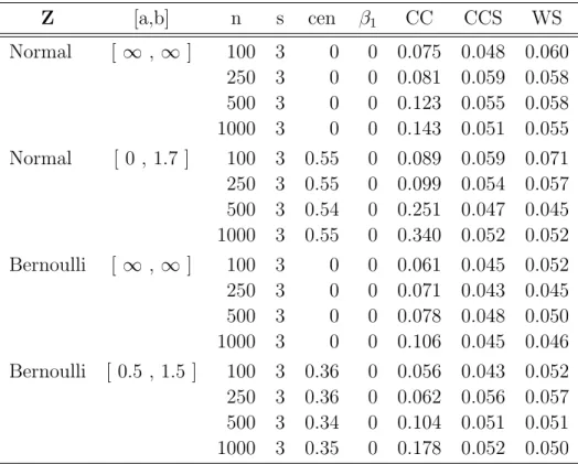
2.1 Comparison of Empirical Sizes of Wald Tests from Censoring Complete (CC), Stratified Censoring Complete (CCS), Stratified Weighted (WS) Estimating Equations (Regularly Stratified Data) . . . 33

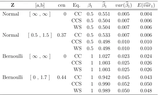
2.2 Comparison of Parameter Estimates from Censoring Complete (CC), Strat-ified Censoring Complete (CCS), StratStrat-ified Weighted (WS) Estimating Equations (Regularly Stratified Data, n= 250) . . . 34

2.3 Comparison of Parameter Estimates from Censoring Complete (CC), Strat-ified Censoring Complete (CCS), and StratStrat-ified Weighted (WSh and WSb) Estimating Equations (Highly Stratified Data) . . . 35

2.4 Estimation of Coefficients and Standard Errors in Models for Breast Can-cer Recurrence . . . 37

2.5 Estimation of Coefficients and Standard Errors in Models for Acute GvHD or Chronic GvHD Occurrence . . . 41

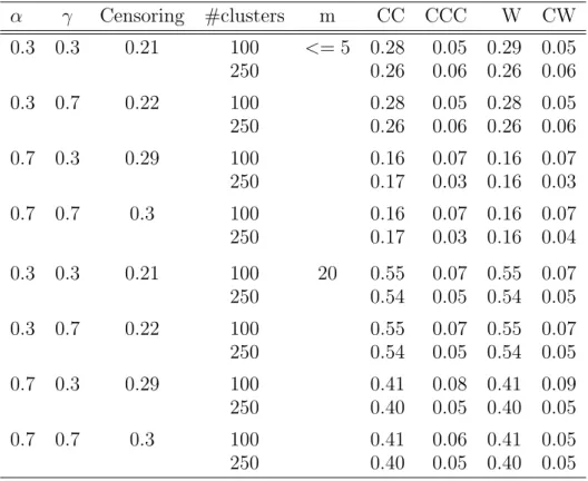
3.1 Comparison of Sizes of Tests with Cluster-constant Covariates . . . 58

3.2 Comparison of Estimators with Cluster-constant Covariates . . . 60

3.3 Estimation of Coefficients and Standard Errors in Models for Acute GvHD or Chronic GvHD Occurrence . . . 62

(12)

Chapter 1 Introduction

1.1 Competing Risks Situation, Endpoints, and

Sum-marizing Functions

In classical survival data, patients can experience the event of interest, or be censored. However, sometimes, patients can have more than one cause of failure; the occurrence of failure from one cause hinders the occurrence of failure from other causes. Three mutually exclusive outcomes are possible in this situation: failure from cause of interest, failure from a competing risk, and censoring without experiencing failure from any cause to last contact. In the sequel, censoring means independent censoring unless dependent censoring or censoring from competing risks is specified.

As with survival analysis, endpoints of interest in the presence of competing risks usually include overall survival (OS) from death from any cause, either with or without the cause of interest, which is the ultimate concern for patients and clinicians; disease free survival (DFS), which is the minimum of time to death and time to event (e.g.

(13)

to independent censoring, such as from loss to follow-up only; therefore, standard analyses would apply. The primary TTE endpoint, however, can be censored by competing causes of failure in addition to the independent censoring, which can make interpretation and analysis difficult.

For example, in studies of treatment for elderly patients with breast cancer, the pri-mary endpoint might be prolonging time to breast cancer recurrence or time to mortality from breast cancer. But some patients may develop other diseases and die without ex-periencing failure of the primary endpoint for the study, thus creating complications for the statistical analysis.

Another example comes from studies of bone marrow transplant, which is a common treatment in leukemia. Graft-versus-host-disease (GvHD) is a problem in this treatment since it can kill patients faster than leukemia itself. The primary endpoint might be time from graft to first occurrence of acute GvHD or chronic GvHD. But death from other causes, such as from leukemia would be competing causes of failure. Patients who are alive without leukemia or GvHD at the end of study are considered to be censored.

In both examples, analysis should explicitly acknowledge the censoring from compet-ing risks since its occurrence and the occurrence of the cause of interest are dependent on each other, unlike the regular independent censoring. Applying classical survival analy-sis to these primary TTE endpoints, i.e. erroneously treating the competing events as censored at the time they occurred, is inappropriate because after a competing event has occurred, failure from the cause of interest is no longer possible. By treating them as censored, we suggest it is still possible; we just no longer observe it.

(14)

LetT denote the failure time;εdenote the cause of failure, andε∈ {1,2, . . . , l};C be the censoring time. On each patient i = 1, . . . , n, we observe the time Xi =min(Ti, Ci),

and the failure status ξi which equals to εi if the subject experienced failure and is 0

when censored.

(1) Latent Failure Times . We assume there exist l mutually exclusive failure types.

{Tej}, j = 1, . . . , l, are latent failure times corresponding to each failure type. Then we

observe T = minj(Tej) and ε = {j : T = Tej} in the absence of censoring. The joint

survival function for Te0

j s

Q(t1, . . . , tl) = Pr(Te1 > t1, . . . ,Tel> tl)

is nonparametrically nonidentifiable from (T, ε), so estimation requires modeling assump-tions. Interpretation of distribution of Tej posits removal of all other causes of failure,

which may not be practically relevant (Prentice et al., 1978). The nonparametric non-identifiability of Q was rigorously established by Tsiatis (1975).

(2)Cause Specific Hazard Function (CSH). The cause-specific hazard for typej failure (or event) is defined as

γj(t) = lim

∆t→0Pr{t ≤T < t+ ∆t, ε=j|T ≥t}/∆t, j = 1, . . . , l.

It simply gives the instantaneous failure rate from cause j at time t treating failures from other causes as censored. An individual’s likelihood contribution (Prentice et al., 1978) is nQ_jγj(t)I(ε=j)

o exp

n

−P_jR₀tγj(s)ds

o

, which factors. So naively disregarding censoring from competing risks leads to valid analysis of the cause-specific hazard function for type j. Standard survival analysis such as Nelson-Aalen estimator, logrank test, and proportional hazards model can be useful. However, the CSH does not capture cumulative failure probabilities of the cause of interest in current reality where other

(15)

events may prevent subsequent occurrence of a causej event. The usual survival function definition for causej: Sj(t) = exp{−

R_t

0 γj(u)du}is no longer the complement to a failure

probability and has no direct clinical interpretation (Pepe and Mori, 1993).

(3) Cumulative Incidence Function (CIF). The cumulative incidence function is an alternative to the CSH. It is also known variously as the cause-specific absolute risk, crude incidence, and cause-specific failure probability. The CIF for cause j at time t is defined as

Fj(t) = Pr(T ≤t, ε =j),

which is the probability of observing an event by time t, and the cause of failure is the event of interest, j. It is not the same as Pr(Tej < t), since ifTek <Tej, andk 6=j, you will

not observe Tej. Fj(∞) is the lifetime risk of cause j event, e.g. recurrence, which may

be less than 1 since the competing risks may intercede before infinity. The CIF can be expressed as a function of the CSH: Fj(t) =

R_t

0 S(u−)γj(u)du, where

S(t) = exp{−R₀tPl_j₌₁γj(u)du} is the overall survival function. Fj may increase either

due to an increase inγj or a decrease inγk, fork 6=j. As an example, the cumulative risk

of breast cancer recurrence may increase either because of increased rate of recurrence or a decreased rate of death prior to recurrence, in CSH.

Alternatively, we can use a hazard-type function, the subdistribution hazard (SH) function directly from the cumulative incidence function for cause j (Gray, 1988):

λj(t) = dFj(t)/{1−Fj(t)}

= lim

∆t→0

1

∆tP{t ≤T ≤t+ ∆t, ε=j|T ≥t∪(T ≤t∩ε6=j)}

The fundamental difference between λj and γj lies in the risk set. The CSH only

(16)

analyses for patients most likely to benefit (suffer) from treatment in absolute terms. (4) Conditional Probability Function(CPF). The CPFj(t) is the probability of

expe-riencing cause j failure by time t conditionally on no competing risks having occurred (Pepe and Mori, 1993). Formally, with two event types (ε= 1,2):

CPF1(t) = Pr(T ≤t, ε= 1|T > t∪ε= 1) =F1(t)/{1−F2(t)}.

For many practitioners, the interpretation of CPFj is straightforward. There are no

implicit assumptions imposed. An issue is that a jump occurs in CPF whenever a failure occurs, not just from the cause of interest. Still, the CPF provides useful complementary information to the CSH/CIF analyses.

The focus of current research is on the direct modeling of the CIF since it is of greatest interest in the applications considered in this thesis. In particular, in both the breast cancer and leukemia studies, the absolute risk of causes of failure is critical when summarizing the effects of treatments.

1.2 Motivating Examples and Objectives

In Section 1.1, we briefly illustrated competing risks problems using a breast cancer trial and a bone marrow transplant study. This current research is motivated by issues encountered in the real data application of these examples. For the reasons discussed earlier, our focus is on the cumulative incidence function.

Clinical trial E1178 conducted by the Eastern Cooperative Oncology Group (ECOG) compared 2 years of tamoxifen therapy to placebo in elderly (≥ age 65) breast cancer patients with positive axillary nodes. In this study, there were 167 eligible patients. Of the 82 patients on placebo, 59 had breast cancer recurrence, 19 died without recurrence, and 4 were censored; of the 85 patients on tamoxifen, 42 had breast cancer recurrence,

(17)

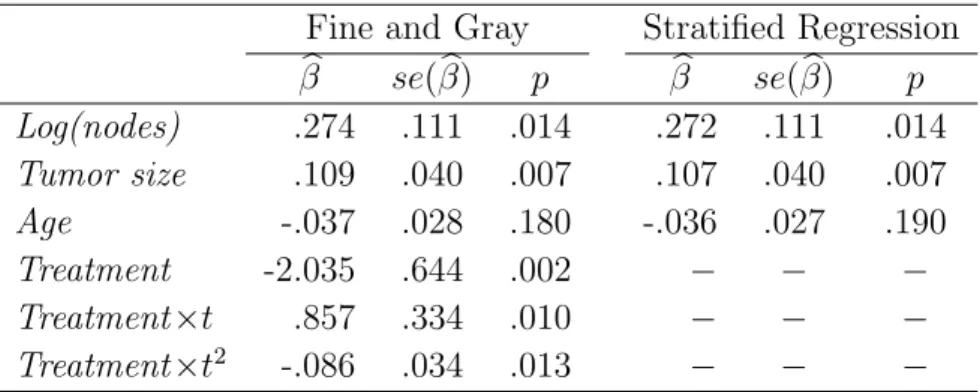
23 died without recurrence, and 20 were censored. In addition to the treatment group to be considered, there were 3 prognostic factors: number of positive nodes, tumor size, and age at treatment. The primary interest is in the absolute risk of the breast cancer recurrence; while death from unrelated causes can be competing risks. The treatment effect on the subdistribution hazard has previously been observed to be non-proportional using regression modeling of the CIF proposed by Fine and Gray (1999) (details are in Section 1.3). We are interested in testing this non-proportionality. We also want to consider a model which adjusts for such discrete factors. For example, with a stratified regression model of the CIF stratifying on treatment, we can test effects of other risk factors. Since there are a large number of patients within each treatment arm, the data are considered regularly stratified.

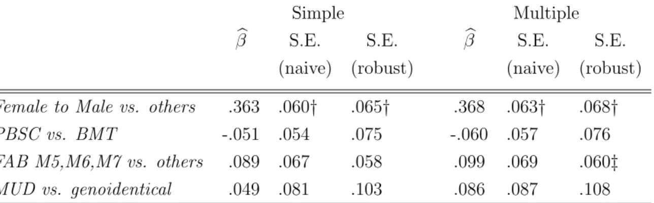
Another example comes from a bone marrow transplant registry provided by the European Blood and Marrow Transplant Group (EBMT). The primary endpoint is time from graft to first occurrence of either acute GvHD grade 2 or chronic GvHD. Death and relapse without GvHD are the competing causes of failure. This is a multicenter design. We have a total of 2996 patients from 244 centers, with 1385 GvHD and 629 competing causes of failure observed. The median follow–up was 1250 days, comprising patients still alive without relapse and disease. The median patients per center was 6 with about 1/3 of centers having only 2 or 3 patients. We are interested in assessing the effect of four prognostic covariates on the primary endpoint, as specified in Katsahian

et al. (2006), where Zik = (Z1ik, Z2ik, Z3ik, Z4ik) for the ith subject in the kth center,

Here Z1ik = I(female donor to male recipient match), Z2ik = I(source of stem cells is

peripheral blood), Z3ik=I(FAB classification of AML is M5, M6, or M7), and Z4ik =

I(type of transplant is matched unrelated donor).

(18)

unobserved center effects may also exist. All of these factors can result in some hetero-geneity across centers and certain within-center correlation. To address this issue, we can either introduce a method that assumes independence among patients conditional on them being in the same center; or we can consider a method that accounts for the potential within-center correlation unconditionally on centers. For the former, Katsahian

et al. (2006) proposed a frailty model for the subdistribution hazard to assess the hetero-geneity across centers and to incorporate such an effect when testing other risk factors. Alternatively, we can consider a stratified regression by stratifying on centers but with-out estimating the center effect. Since the number of centers is much larger than center sizes, we have highly stratified data. Which method to choose ultimately depends on the design of the study or/and scientific interest. If the data were stratified by design, a stratified approach makes sense. If the scientific interest is more on the study population, then a model for clustered competing risks may be more appropriate. Both approaches are studied in this thesis.

1.3 Existing Methods for the Analysis of Competing

Risks Data

1.3.1 Univariate Models for Cumulative Incidence Functions

There have been various nonparametric and semiparametric methods proposed for mod-eling the cumulative incidence function Fj(t). In the sequel, we assume cause 1 is the

cause of interest. In order to compare the cumulative incidence of a particular type of failure amongstK different groups, Gray (1988) developed a class of K-sample tests based on weighted averages of the subdistribution hazards for cause 1: λ1(t). Pepe proposed a

nonparametric two-sample generalized test for comparing g(F1(t), . . . , Fl(t)), where g is

a smooth function (Pepe, 1991). Both methods only consider discrete factors.

(19)

When analyzing cause-specific failure patterns, investigators may be interested in the effects of covariates on the event-specific failure probabilities. Such analyses may involve testing the effects of treatment adjusted for important prognostic factors, in addition to testing the effects of the prognostic factors (Jeong and Fine, 2007).

Suppose we observe covariates Z, which is a r × 1 vector on each patient. The cumulative incidence function for failure from cause 1, conditional on the covariates, is F1(t;Z)≡P r(T ≤ t, ε= 1|Z). Similarly, other functions defined in Section 1.1, such as

the cause-specific hazardγ1(t), the subdistribution hazardλ1(t), the overall survivalS(t),

and S1(t), become γ1(t;Z), λ1(t;Z), S(t;Z),and S1(t;Z) respectively, conditional on Z.

Simply fitting a Cox proportional hazards model for cause 1 does not give the covariate effects on F1(t;Z); it only gives the effects onγ1(t;Z), and hence on S1(t;Z) (Prenticeet

al., 1978; Cox, 1972).

To conduct regression analysis of the cumulative incidence function, the cause-specific hazards approach is still applicable by fitting a Cox regression model to each of the l cause-specific hazards and treating failure from other causes as censored: γj(t;Z) =

γj0(t) exp(α0j0Z) with baseline hazard γj0(t) and regression coefficient αj0, j = 1, . . . , l.

We then obtain the cumulative incidence of cause 1 by F1(t;Z) =

R_t

0 S(u;Z)γ1(u;Z)du.

This approach can be restrictive in some sense since we need to assume proportional hazards of covariate effects for all other cause-specific hazards in addition to cause 1. The covariate effects onF1 not only depend on their effect on γ1, but also on their effect

on all γj, j 6= 1. Therefore, the resulting cumulative incidence functions are somewhat

(20)

due to an increase in γ1 or a decrease in γj, for j 6= 1. For example, if an increase in Z

increases γ1, but also increases γ2 by much more, then F1 may decrease since subjects

are likely to fail from cause 2 first.

Fine and Gray (1999) proposed a semiparametric proportional subdistribution haz-ards model to directly assess the effect of covariates or prognostic factors on the cu-mulative incidence function. By working with the subdistribution hazard λ1(t;Z), their

approach avoids modeling other causes of failure. The model relates the covariates to λ1(

·

) by assuming

λ1(t;Z) =λ10(t) exp(β00Z),

whereλ10(

·

) is an unspecified, nonnegative function denoting the baseline subdistribution

hazard when covariate Z =0; β0 is a r×1 vector of unknown regression parameters; Z

is allowed to include time-varying covariates which are known, deterministic functions of time and time-independent covariates, hence fully observed. In the sequel, we suppress the dependence on time, when there is no loss of clarity. This corresponds to a propor-tional hazards model forT∗ ₌_I(ε_{= 1)}_×_T ₊_I(ε₆_{= 1)}_{× ∞}_{. Thus, the Fine–Gray model}

is a Cox model analogue for competing risks failure time data.

More recently, Fine (2001) extended the Fine–Gray model to a more general semi-parametric transformation model for the cumulative incidence function of a competing risk, conditional on covariates, which is not based upon the subdistribution hazard. The model is in the form of g{F1(t;Z)} = h(t)−Z0β. g(x) = log{−log(1−x)} gives the

proportional subdistribution hazards model; and g(x) = logit(x) gives a proportional odds model (logistic regression). The estimation of regression coefficients is achieved with a rank-based least squares criterion, which is different from the Fine–Gray model. It is less efficient under the proportional subdistribution hazards model; but is more flexible.

Alternative models and methods of estimation for cumulative incidence regression

(21)

have been studied in, for example, Klein and Andersen (2005), Scheike and Zhang (2008), and Scheike, Zhang, and Gerds (2008), including nonproportional hazards models and goodness-of-fit methods for assessing the proportional subdistribution hazards assump-tion. In particular, Scheike, Zhang, and Gerds (2008) proposed a direct binomial re-gression for F1(t;Z), which is an extension of Fine’s (2001) transformation model. The

models are flexible, but not as efficient when there is heavy censoring. Jeong and Fine (2006) proposed a direct parameterization of the cumulative incidence function without covariates. Jeong and Fine (2007) extended it to the parametric regression setting, which adopts the likelihood-based parametric analyses for the cumulative incidence function as a practically useful alternative to semiparametric methods.

Although these new developments in competing risks regression are very flexible, the Fine–Gray model continues to be the most popular direct regression modeling method for the cumulative incidence function due to it being a natural adaptation to the cause-specific hazards model and a Cox model analogue for competing risks data.

1.3.2 Extended Models for Cumulative Incidence Functions and

Multivariate Survival Models

(22)

naive application of the Fine–Gray model, either omitting such covariates or including them assuming they satisfy the proportional hazards assumption, could lead to biased estimation and tests, and potential loss of power.

Existing work on the cumulative incidence function that account for such issues has taken several forms:

(1) Modified nonparametric Gray-type tests (Chen et al., 2008). The tests focus on formally testing group effects, which limits the introduction of continuous covariates and quantification of covariate effects.

(2) Mixed proportional subdistribution hazards models (Katsahian et al., 2006). This is a frailty regression model (Vaupel et al., 1979; Hougaard, 1984) tailored to competing risks failure time data. Although the approach seems promising, the performance of the proposed frailty model and estimators were assessed through simulations and the statistical properties are unclear (Katsahian et al., 2006). Moreover, in situations where the main goal is to investigate covariate effects, introducing a dependence parameter in modeling the joint distribution within each cluster does not seem to have much advantage compared to any model whose dependence structure is unspecified (Lee, Wei and Amato, 1992).

(3) Introducing interactions using time-dependent covariates to the Fine–Gray model

(Fine and Gray, 1999). Introducing time-dependent covariates to the Fine–Gray model to capture cluster effects complicates the model and the explanation of the non-cluster covariate effects.

(4) Multiple imputation (Ruan and Gray, 2008). Recently, Ruan and Gray proposed a generic Kaplan-Meier multiple imputation method that recovers the missing potential censoring information for the analysis of cumulative incidence functions using standard analysis, which can potentially be applied in the setting of stratified analysis. Although the methods perform well empirically, the statistical properties of the approach are not

(23)

established. Such imputation-based procedures have not been used very often in survival settings, in part because of the ad hoc nature of the resulting inferences and a lack of understanding regarding when such inferences are valid.

Various other analytic strategies used widely in classical survival analysis, however, have not been adopted to competing risks setting. Notably, stratification is a standard approach to account for varying patient populations such as in multicenter clinical trials, where baseline hazards vary across centers (Therneau and Grambsch, 2000). Stratifi-cation on the non-proportional factors may yield a simpler and more flexible analysis than modeling interactions parametrically with functions of time through defined time-dependent covariates (Kalbfleisch and Prentice, 2002). No paper on stratified Cox model was found/needed in the literature since the stratification can be achieved by adding a sum over strata in all expressions from the Cox model for each stratum. The analysis can be realized through survival analysis software in SAS, Splus, or R convenient with an option for the strata. This stratified method is specified conditionally on strata, where subjects are assumed to be independent within each stratum.

There is another approach which specifies proportional subdistribution hazards model unconditionally on strata, and thus induces dependence amongst subjects within each stratum. These are called marginal models, which formulate the marginal distributions of multivariate (correlated) failure time data. Wei, Lin and Weissfeld (1989) proposed a marginal model with distinguishable baseline hazard functions among distinct failure types: γik(t) = γ0k(t) exp{βk0Zik(t)}, where i denotes the patients and k denotes the

type of event. Lee, Wei and Amato (1992), Liang et al. (1993), and Cai and Prentice (1997) proposed various marginal models with a common baseline hazard function, where γik(t) = γ0(t) exp{β0Zik(t)}. Spiekerman and Lin (1998) proposed a marginal mixed

(24)

type.

Although both stratified analysis and marginal model may apply to data with large numbers of small groups (highly stratified data), they can differ in many ways in terms of model formulation, power of tests, interpretation, and, most importantly, the scientific questions of interest. The choice between the two analytical models can depend on what scientific questions are of interest. Sometimes the analysis approach is dictated by the study design: if we stratify the design, then a design based analysis would be stratified as well. The covariate effects in the conditional model can be attenuated by the frailty. In addition, the regression coefficients in a marginal model describe the effects of covariates on the population mean response. Its interpretation does not depend on assumptions made on the within-cluster association. The regression coefficients of the stratified model have stratum-specific interpretation instead of the population mean.

Neither the stratified nor marginal approach has been proposed or used in the analysis of competing risks failure times for cumulative incidence functions. In current research, we develop rigorous methodology for stratified and marginal Fine–Gray models for com-peting risks data, similar to the methodology typically employed with stratified and marginal Cox models for independently censored data.

1.3.3 Goodness-of-fit Tests for Cumulative Incidence Models

In classical survival analysis, the hazards are assumed to be proportional in the Cox model. Violation of the assumption may have adverse effect on the statistical inference,

e.g., lead to distortion of the size and reduction of the power of the partial likelihood score test (Lagakos and Schoenfeld, 1984; Lagakos, 1988; Lin and Wei, 1989; Lin and Wei, 1991). Similarly, the same issues may exist in the Fine–Gray model when the proportional subdistribution hazards (PSH) assumption is violated.

Graphical and analytical methods can be used in checking the PSH, so that approaches

(25)

can be taken to change the model in the direction of the non-proportionality, e.g., strat-ification, time-dependent covariates, etc. However, this has received little attention in the literature. Scheike and Zhang (2008) proposed to test PSH in their direct binomial model of the CIF. Dauxois and Kirmani (2004) proposed testing the proportionality of the two CIF instead of the subdistribution hazards. Formal numerical tests have yet to be developed for the Fine–Gray model.

In contrast, various goodness-of-fit tests have been proposed to test the proportional hazards assumption in the Cox model. Cox (1972) proposed to check the model by intro-ducing a dummy time-dependent covariate. Schoenfeld (1980), Moreau, O’Quigley and Mesbah (1985), and Moreau, O’Quigley, and Lellouch (1986) proposed tests by partition-ing the subjects into mutually exclusive regions based on the values of the covariates and time axis. There are tests based on weighted sums of the martingale residuals, e.g. in Barlow and Prentice (1988), Lin et al. (1993), Gronnesby and Borgan (1996) and Marzec and Marzec (1997). There are also tests based on Schoenfeld residuals and score process, among which, the tests based on weighted residuals proposed by Grambsch and Therneau (1994) are most widely cited and are very straightforward and easy to use in practice. By extending the Cox model to include time varying coefficients, a time-weighted score test on those covariates can be conducted. It is this method that will be extended in the current work.

1.4 Proposed Methods and Outline

(26)

where the number of groups (strata) is large compared to the strata sizes. The ECOG data and the EBMT data are examples of each regime respectively.

For the clustered competing risks failure time data, a marginal proportional subdis-tribution hazards model is proposed, which is similar to Lee, Wei and Amato (1992)’s marginal model, except that we focus on subdistribution hazards instead of the cause-specific hazards. Under the independence working assumption, the cumulative incidence function and the effects of the prognostic factors can be estimated by following the Fine– Gray methodology, while accommodating the correlation within clusters.

The difference in the stratified and marginal models are essentially similar to that in classical survival analysis which has been discussed in Section 1.3.2.

In Section 2.1 we introduce the stratified Fine–Gray model. In Section 2.2 we dis-cuss partial likelihood inferences for the stratified model in the absence of independent censoring, along with inverse weighting estimation equations which permit independent censoring. Asymptotic properties of these procedures are presented in Section 2.3, with results for the two stratification regimes in separate subsections. The prediction of cumu-lative incidence is discussed in Section 2.4. Section 2.5 discusses some simulation studies, with the analysis of the two motivating data sets following in Section 2.6.

Section 3.1 introduces the marginal Fine–Gray model for clustered data. In Section 3.2 we discuss pseudo partial likelihood inferences for the marginal model. As for the stratified case, inverse weighting estimation equations are used in the presence of inde-pendent censoring. Asymptotic properties of these procedures are then presented. The prediction of cumulative incidence is described in Section 3.3. Section 3.4 gives a scheme of generating clustered competing risks data and assesses the performance of our pro-posed model through some simulation studies. The application of the propro-posed method to the motivating data (EBMT) follows in Section 3.5.

In Chapter 4, we propose a proportional subdistribution hazards (PSH) test for the

(27)

Fine–Gray model. Section 4.1 reviews the Fine–Gray model and discusses model exten-sions for assessing lack of fit. In Section 4.2, we discuss the goodness-of-fit test using the extended model. A score test statistic for PSH is proposed based on Grambsch and Therneau (1994) and studied theoretically. The proposed methods are examined through simulation studies in Section 4.3. Its application to the ECOG data is shown in Section 4.4. We conclude the chapter with a brief discussion in Section 4.5.

(28)

Chapter 2 Competing Risks Regression for

Stratified Data

2.1 Data and Model

For stratified competing risks data, we assume the subjects are independent given their membership, that is, conditional on stratum. We observe {Xik = (Tik ∧Cik), ∆ik =

I(Tik ≤ Cik), ξik = ∆ikεik, Zik} for i= 1, . . . , s; k = 1, . . . , mi, where i denotes the

stratum, k denotes the subject within the stratum, and Ps_i₌₁mi =n. Here, the random

variables Tik, Cik, εik,Zik are defined analogously to those in Chapter 1. For regularly

stratified data, we assume i.i.d. observations within strata, while for highly stratified data, we assume that information observed within each stratum is i.i.d. across strata; see Assumption 2.1 in Section 2.2.

For the event of interest (cause 1), we define the cumulative incidence function for stratum i as F1i(t;Zik) ≡ Pr(Tik ≤ t, εik = 1|Zik). Correspondingly, the

(29)

dF1i(t;Zik)/{1−F1i(t;Zik)}is

λ1i(t;Zik) =λ1i0(t) exp(β00Zik), (2.1)

where λ1i0 is the baseline subdistribution hazard in stratum i = (1, . . . , s) and β0 is the

regression coefficient, which is assumed common to all strata. An important point is that no assumptions are made about the relationships between the baseline hazard functions. When appropriate, all the observations can be denoted using single index without the index for stratum: {Xl, ∆l, ∆lεl, Zl, Sl}, wherel = 1, . . . , n is an index for all subjects

in the entire data set, andSl denotes the stratum for lth observation.

2.2 Estimation

The estimation procedure is adapted from Fine and Gray (1999). Inheriting their notation and terminology, we call the data complete when failure timeTik and failure cause εik are

observed for all individuals; we call the data censoring complete when the failure time is right censored but potential censoring time Cik is always observed. Starting from a

modification of the partial likelihood for the subdistribution for complete or censoring complete data, we then extend the estimation equation to classical right censored data, where eitherTik orCik is observed, but not both.

We assume there exists a τ and δ such that Pr(Tik > τ) > δ > 0,Pr(Cik = τ) =

Pr(Cik ≥ τ) > δ > 0 for all i, k. This assures, essentially, at least a proportion of

subjects survive to time τ and all the subjects surviving past τ are censored at τ . Let Nik(t) = I(Tik ≤ t, εik = 1) and Yik(t) = 1 −Nik(t−) denote the counting

process and risk process respectively for the complete data. When the data are censoring complete, the risk process is modified to Y∗

ik(t) = I(Cik ≥ t)Yik(t). I(Cik ≥ t) is an

(30)

other causes are excluded from the risk set at their (potential) censoring times. Thus Y∗

ik(t) equals to 0 if the subject failed from the event of interest or is censored by time

t, and 1 otherwise. When the data are right censored, the implicit weight is changed to weight wik, which is explained in detail in Section 2.2.2.

For convenience, the following notation is introduced:

S(_ip)(β, t) =m−1

i mi X

k=1

Y∗

ik(t)Zik(t)⊗peβ

0_Z

ik(t)_, _p_{= 0,}_1,_2,

Zi(β, t) =S(1)i (β, t)/S

(0)

i (β, t), i= 1, . . . , s,

s(_ip)(β, t) = lim

mi→∞ m−1

i mi X

k=1

Y∗

ik(t)Zik(t)⊗peβ

0_Z

ik,

ei(β, t) =s(1)i (β, t)/s

(0)

i (β, t),

vi(β, t) =s(2)i (β, t)/s(0)i (β, t)−e⊗i 2(β, t),

b

S(_ip)(β, t) =m−1

i mi X

k=1

b

wik(t)Yik(t)Zik(t)⊗peβ

0_Z

ik(t)_, b

Zi(β, t) =Sb

(1)

i (β, t)/Sb

(0)

i (β, t),

e

S(_ip)(β, t) =m−1

i mi X

k=1

wik(t)Yik(t)Zik(t)⊗peβ

0_Z

ik(t), e

Zi(β, t) =Se

(1)

i (β, t)/Se

(0)

i (β, t).

with a⊗0 _{= 1,}_a⊗1 ₌_{a, and} _a⊗2 ₌_aa0_.

Assumption 2.1 The following list of conditions are assumed throughout the chapter: C1. R₀τλ1i0(t)dt <∞.

C2. Zaik(

·

)(i= 1, . . . , s;k = 1, . . . , mi) have bounded total variations, i.e. for ath

compo-nent of Zik, a= 1, . . . , d, |Zaik(0)|+

R_τ

0 |dZaik(t)| ≤M, where M is a constant.

C3. {Nik(

·

), Yik(

·

),Zik(

·

), mi, k = 1, . . . , mi}fori= 1, . . . , sare independently distributed

(31)

for regularly stratified data; and i.i.d for highly stratified data. Under both types of strat-ification, {Nik(

·

), Yik(

·

),Zik(

·

)}k=1,...,mi are i.i.d within each stratum i.

C4. Regularity conditions for different regimes:

• For regularly stratified data, there exists a neighborhood B of β0 and scalar, vector

and matrix functionss(0)_i , s(1)_i ands_i(2) defined onB ×[0, τ]such that for p= 0,1,2, sup_t_∈_[0_,τ_]_,β_∈BkS(_ip)(β, t)−s(_ip)(β, t)k−→p 0. ThenΩri =

R_τ

0 vi(β0, t)s (0)

i (β0, t)λ1i0(t)dt

is positive definite for each i.

• For highly stratified data, both

Ωh ≡ lim

n→∞n

−1

s

X

i=1

E "_m

i X

k=1

Z _τ

0

{Zik(u)−Zi(β0, u)}⊗2Yik∗(u)eβ

0

0Zik(u) dNi(u) S(0)_i (β0, u)

#

for censoring complete case and

e

Ωh ≡ lim

n→∞n

−1

s

X

i=1

E "_m

i X

k=1

Z _τ

0

{Zik(u)−Zei(β0, u)}⊗2wik(u)Yik(u)eβ

0

0Zik(u) dNi(u) e

S(0)_i (β0, u)

#

for right censored case are positive definite.

2.2.1 Complete and Censoring Complete Data

With complete data, the risk set associated withλ1i at time of failure for thekth subject

in the ith stratum is defined as: Rik = {k0 : (Tik0 ≥ T_ik)∪(T_ik0 ≤ T_ik ∩ ε_ik0 6= 1)}.

When the data are censoring complete, the associated risk set is modified to Rik ={k0 :

(Tik0 ∧C_ik0 ≥T_ik)∪(T_ik0 ≤T_ik∩ ε_ik0 6= 1∩C_ik0 ≥ T_ik)}. We will detail the derivation

of the partial likelihood approach for the censoring complete data, since the complete data are special cases of the censoring complete data by letting the censoring times to be larger than the maximum failure time.

(32)

partial likelihood

L∗_{(β) =}

s

Y

i=1

mi Y

k=1

½

eβ0_Z

ik(Xik) P_m_i

k0₌₁Y_ik∗0(X_ik)eβ 0_Z

ik0(Xik)

¾∆ikI(εik=1)

=

s

Y

i=1

mi Y

k=1

( eβ0_Z

ik(Xik) miS(0)i (β, Xik)

)_∆_ik_I₍_ε_ik₌₁₎

. (2.2)

Differentiating the log partial likelihood with respect toβ produces the estimating equa-tion that can be expressed in a counting process formulaequa-tion as

U∗₁(β, t) =

s

X

i=1

mi X

k=1

Z _t

0

©

Zik(u)−Zi(β, u)

ª

I(Cik ≥u)dNik(u). (2.3)

The estimatorβ, which maximizesb L∗_{(β) may be obtained as a solution to}_U∗

1(β, τ) = 0.

2.2.2 Weighted Estimating Equation for Right Censored Data

When classical right censoring is present, we can adapt inverse probability of censoring weighting (IPCW) techniques (Robins and Rotnitzky, 1992) to construct an unbiased estimating function, as proposed by Fine and Gray (1999). Let G(

·

) be the survival function of the censoring variable with highly stratified data andGi(

·

) in theith stratum

with the regular stratification. For regularly stratified data, the implicit weightI(Cik ≥t)

with the censoring complete data is replaced bywik(t) =I(Cik ≥Tik∧t)Gi(t)/Gi(Xik∧t),

andGi(t) = P r(Cik ≥t), k = 1, . . . , mi, for eachi, assuming the distribution of censoring

time is stratum-dependent. For highly stratified data, the replacement would bewik(t) =

I(Cik ≥ Tik∧t)G(t)/G(Xik ∧t), and G(t) = P r(Cik ≥ t), i = 1, . . . , s;k = 1, . . . , mi,

assuming random vectors (mi, Ci1, ..., Cimi) are i.i.d. across i, but allow dependence in the censoring times among patients in a given stratum. That is, arbitrary dependence among Ci1, ..., Cimi would be allowed.

(33)

The difference in the assumptions for the two data regimes has to do with the consis-tency of the potential estimator of the censoring time distribution. For regularly stratified data, the size of each stratum goes to infinity. We can afford to allow for the dependence between the censoring times and the strata. Therefore, Gi(

·

) is used. If strata sizes are

finite, we cannot consistently estimate the censoring distribution in each stratum. Infor-mation must be pooled across strata via the assumption of a single G, as is employed with highly stratified data.

Since the distribution of the censoring random variable is unknown in either stratifi-cation regimes, theGi(

·

) (G(

·

)) need to be estimated: Gbi(

·

), the Kaplan-Meier estimator

of the survival function of the censoring random variable in theith stratum is used with regular stratification andG(b

·

), the Kaplan-Meier estimator of the survival function of the censoring random variable, is used with high stratification. Only patients from the ith stratum are used in the calculation of Gbi for regularly stratified data since the stratum

sizes go to infinity. In contrast, for highly stratified data, patients from all strata are used in G.b

The estimated weights are wbik(t) = I(Cik ≥ Tik ∧t)Gbi(t)/Gbi(Xik ∧t) or wbik(t) =

I(Cik ≥Tik∧t)G(t)/b G(Xb ik∧t) such thatwbik(t)→wik(t) asn → ∞for both stratification

regimes. That is,

b wik(t) =

     

    

0 if Xik < t, ξik = 0

b

Gi(t|Xik) or G(tb |Xik) if Xik < t, ξik >0

1 if Xik ≥t ,

b

wik(t)Yik(t) =

     

    

0 if Xik < t, ξik ≤1

b

Gi(t|Xik) or G(tb |Xik) if Xik < t, ξik >1

(34)

The resulting weighted score function is:

U1(β, t) =

s X i=1 mi X k=1 Z _t 0 ½

Zik(u)−

P_m_i

k0₌₁wbik0(u)Y_ik0(u)Z_ik0(u)eβ 0_Z

ik0(u) P_m_i

k0₌₁wb_ik0(u)Y_ik0(u)eβ0Zik0(u)

¾ b

wik(u)dNik(u)

= s X i=1 mi X k=1 Z _t 0 n

Zik(u)−Zbi(β, u)

o b

wik(u)dNik(u), (2.4)

The estimator of β is obtained by zeroing the estimating equation (2.4).

2.3 Inference

In this section, we consider the asymptotic properties of the estimators for different data regimes. In each case, the consistency ofβbcomes first. Then the asymptotic normality of n−1₂_U∗

1(β0, τ) (orn−

1

2U₁(β₀, τ) for right censored data) is shown. Asymptotic normality

of n12(βb− β₀) is obtained by Taylor series approximation using the first two results.

Variance estimation follows.

2.3.1 Regularly Stratified Data

In this scenario, the number of strata s is finite. When n → ∞, mi → ∞, for each

i= 1, . . . , s. We use the subscript r to denote the regularly stratified case.

We start from the censoring complete data. Under the conditions stated in Section 2.2, we can show thatβbis consistent by adapting the consistency result ofβbin Andersen and Gill (1982). Then by Taylor series expansion and the consistency of β,b n12(βb−

β0)≈Ω−r1{n−

1 2U∗

1(β0, τ)}, where Ωr is the limit of the negative of the partial derivative

matrix of the score functionU∗

1(β, τ) evaluated atβ0. Clearly,U∗1(β, t) =

P_s

i=1U∗1i(β, t),

where each component U∗

1i(β, t) =

P_m_i

k=1

R_t

0

©

Zik(u)−Zi(β, u)

ª

I(Cik ≥ u)dNik(u) can

be viewed as a separate estimation equation for censoring complete data in the Fine– Gray model. Adding the stratum specification - subscript i to their results, we can see

(35)

as mi → ∞, m−

1 2

i U∗1i(β0, τ)−→D N(0,Ωri) with

Ωri =

Z _τ

0

{s(2)_i (β0, t)/s(0)i (β0, t)−ei(β0, t)⊗2}s(0)i (β0, t)λ1i0(t)dt,

SinceΩri is the limit of the negative of the partial derivative matrix of the score function

U∗

1i(β, τ) evaluated at β0, at the limit,

P_s

i=1πiΩri = Ωr, where pi = mi/n → πi.

Asymptotic normality results for censoring complete data are thus obtained: as n → ∞, n−1₂_U∗

1(β0, τ) =

P_s

i=1p

1 2

im

−1 2

i U∗1i(β0, τ) −→D N(0,Ωr). Hence, n−

1

2(βb− β₀) −→D

N(0,Ω−1

r ).

A consistent estimate of the covariance matrix for the regression coefficients can be obtained by replacing the unknown quantities with their observed values. We have

b Ωr =

1 n s X i=1 mi X k=1

∆ikI(εik = 1)



S(2)i (β, Xb ik)

S(0)_i (β, Xb ik)

−

(

S(1)_i (β, Xb ik)

S(0)_i (β, Xb ik)

)_⊗₂

_. _(2.5)

When the data are right censored, by applying results for weighted score function of incomplete data (Fine and Gray, 1999) to each component of U1(β, t): U1i(β, t) =

mi X

k=1

Z _t

0

{Zik(u) −Zbi(β, u)

o b

wik(u)dNik(u) and modifying the results for censoring

com-plete data, the asymptotic properties for right censored stratified data are obtained as follows.

Lemma 2.1 (Consistency of β)b . βb−→p β0 for right censored regularly stratified data.

Proof: First, for eachi,m−_i 1{U1i(β, τ)−U∗1i(β, τ}converges in probability to 0 uniformly

for β in a compact neighborhood of β0 (Fine and Gray, 1999). It follows that as n → ∞, n−1_{_U

1(β, τ)−U∗1(β, τ)}=

s

X

i=1

pim−i 1{U1i(β, τ)−U∗1i(β, τ)}converges in probability

to 0 uniformly for β in a compact neighborhood of β0. Therefore, β, the solution tob

(36)

Theorem 2.1 (Asymptotic normality of U1(β0, τ)). n−

1

2U₁(β₀, τ)−→D N(0,Σ_r)for right

censored regularly stratified data, the details of the Σr is in the proof below.

Proof: For each i, m−12

i U1i(β0, τ)−→D N(0,Σri), where

Σri = E

©

(η_ik+ψ_ik)⊗2ª_.

The details of η_ik and ψ_ik for each i are omitted here since they are the same as η_k and ψ_k in Fine–Gray model except for adding the subscript i. From this point, it is straightforward that n−1

2U₁(β₀, τ) = Ps

i=1p

1 2

im

−1₂

i U1i(β0, τ) is asymptotically normally

distributed asN(0,Σr), where Σr =

P_s

i=1πiΣri.

Theorem 2.2 (Asymptotic normality of β)b . n12(βb−β₀)−→D N(0,Ω−1

r ΣrΩ−r1) for right

censored regularly stratified data.

Proof: Similar to the censoring complete situation, n12(βb−β₀) ≈ Ω−_r1{n− 1

2U₁(β₀, τ)},

whereΩ−_r1 has the same form as the variance of the stratified censoring complete regres-sion coefficients. Hence, the distribution of n12(βb−β₀) is asymptotically normal with

covariance matrix Ω−1

r ΣrΩ−r1.

In order to estimate the covariance matrix for the regression coefficients, we need to find a consistent estimator ofΩrandΣr. The estimator ofΩrisΩbrin Equation (2.5) with

b

S(_ip) replacing S(_ip) for each i, p= 0,1,2. Each component of Σr, Σri, can be estimated

with the empirical covariance matrix Σbri =m−i 1

P_m_i

k=1(bηik+ψbik)⊗2. For brevity, we do

not show the details ofηb_ikandψb_ik, which can be obtained by adding subscriptktoηb_i and b

ψ_iin Fine and Gray (1999). Therefore, the distribution ofn12(βb−β₀) can be approximated

by a normal distribution with variance n{Ps_i₌₁miΩbri}−1{

P_s

i=1miΣbri}{

P_s

i=1miΩbri}−1.

(37)

2.3.2 Highly Stratified Data

In this scenario, the strata size mi is finite, i = 1, . . . , s. s → ∞ as n → ∞. We use

subscript h for some quantities to denote the highly stratified case.

As in the regularly stratified data, we consider the censoring complete situation first.

Lemma 2.2 (Consistency of β)b . βb−→p β0 for censoring complete highly stratified data.

Proof: The technical details are in Appendix A.1.

Theorem 2.3 (Asymptotic normality of U∗₁(β0, τ)). n−

1

2U∗₁(β₀, τ) −→D N(0,Ω_h) for

censoring complete highly stratified data. Proof: SinceM∗

ik(β, t) =

R_t

0 I(Cik ≥u)dNik(u)−

R_t

0Yik∗(u)λ1i0(u)eβ 0_Z

ik(u)duis a martingale for censoring complete data filtration F∗_{(t) =} _σ_{_I(C

ik ≥ u), I(Cik ≥ u)Nik(u), Yik∗(u),

Zik(u), u ≤ t, i = 1, . . . , s;k = 1, . . . , mi} (Fine and Gray, 1999), we can reexpress

U∗₁(β, t) as a martingale type estimation equation:

U∗

1(β, t) =

s

X

i=1

mi X

k=1

Z _t

0

©

Zik(u)−Zi(β0, u)

ª dM∗

ik(β, u).

Applying the martingale central limit theorem (Rebolledo, 1980),n−1 2U∗

1(β0,

·

) converges

in distribution to a continuous Gaussian process. At time t = τ, n−1 2U∗

1(β0, τ) −→p

N(0,Ωh), whereΩh is defined in Assumption 2.1. That is because the covariance matrix

equals to

lim

n→∞n

−1

s

X

i=1

E " _m

i X

k=1

Z _τ

0

{Zik(u)−Zi(β0, u)}⊗2Yik∗(u)eβ

0

0Zik(u)_λ

1i0(u)du

# ,

which is equivalent toΩh, the limit of the negative of the partial derivative matrix of the

score function U∗

(38)

Theorem 2.4 (Asymptotic normality of β)b . n−1₂₍_βb₋_β

0) −→D N(0,Ω−h1) for censoring

complete highly stratified data.

Proof: This is a direct result of Lemma 2.2, Theorem 2.3, and the fact thatn12(βb−β₀)≈

Ω−_h1{n−1

2U∗₁(β₀, τ)}.

By replacing the unknown quantities in Ωh with their observed values. We have

b Ωh =

1 n s X i=1 mi X k=1

∆ikI(εik = 1)



S(2)i (β, Xb ik)

S(0)_i (β, Xb ik)

−

(

S(1)_i (β, Xb ik)

S(0)_i (β, Xb ik)

)_⊗₂ _,

exactly the same formulation as Ωbr in equation (2.5).

The properties of the estimator for right censored highly stratified data follow:

Lemma 2.3 (Consistency of β)b . βb−→p β0 for right censored highly stratified data.

Proof: For technical details, please refer to Appendix A.2. Theorem 2.5 (Asymptotic normality of U1(β0, τ)). s−

1

2U(β₀, τ)−→D N(0,Σ_h)for right

censored highly stratified data.

Proof: The details are shown in Appendix A.3.

The covariance matrix Σh = E{(ηi+ψi)⊗2}, where

ψ_i =

mi X

k=1

Z _∞

0

q(y)/{mπ(y)}dM_ikc(y),

η_i =

mi X k=1 Z _t 0 n

Zik(u)−Zei(β0, u)

o

wik(u)dNik(u),

π(y) = lim

n→∞ 1 n n X l=1

I(Xl ≥y),

q(y) = E " _m i X j=1 mi X k=1 Z _t 0

Aij(β0, u)I(Xij < y ≤u)wij(u)wik(u)dNik(u)

# , and

Aij(β0, u) =

Yij(u)eβ

0

0Zij(t) nSe(0)_i (β0, u)

×

n

Zij(u)−Zei(β0, u)

o .

(39)

Here,j is an index for patients within each stratum (likek) andZei(β0,

·

) isZbi(β0,

·

) with

b

wik(

·

) being replaced by wik(

·

), Mikc(

·

) is the martingale associated with the censoring

process, and Λ1i0(

·

) is the baseline cumulative hazard forith stratum.

Theorem 2.6 (Asymptotic normality of β)b . n12(βb−β₀)−→D Ωe

−1

h (m−1Σh)Ωe

−1

h for right

censored highly stratified data.

Proof: Similar to Theorem 2.2, n12(βb−β₀)≈Ωe

−1

h {n−

1

2U₁(β₀, τ)}, where Ωe_h is the limit

of the negative of the partial derivative matrix of the score function U1(β, τ) evaluated

atβ0. Hence, by Lemma 2.3 and Theorem 2.5, n

1

2(βb−β₀) is asymptotically normal with

covariance matrix Ωe−_h1(m−1_Σ

h)Ωe

−1

h .

The estimator of Ωeh is Ωbh with Sb

(p)

i replacing S

(p)

i for all i and p as in the regularly

stratified case. The inner matrix in the variance, Σh, can be estimated empirically by

1/sPs_i₌₁(bη_i+ψb_i)⊗2_, _where

b η_i =

mi X k=1 Z _∞ 0 n

Zik(u)−Zbi(β, u)b

o b

wik(u)dNik(β, u),b

b ψ_i =

mi X k=1 Z _∞ 0 b

Q(β, y)b (

n

X

l=1

I(Xl≥y)/s

)₋₁ dMcc

ik(y),

c

Mc_{(y) =}_I(X _≤_y,_{∆ = 0)}₋

Z _y

0

I(X ≥t)dΛbc_(t),

b Λc(t) =

Z _t

0

( _n X

l=1

I(X ≥y)

)₋₁ _n X

l=1

dI(X ≤u,∆ = 0),

b

Q(β, y) =b s−1

s X i=1 mi X j=1 mi X k=1 Z _∞ 0 b

Aij(β, u)I(Xb ij < y ≤u)wbij(u)wbik(u)dNik(u),

and Abij is defined analogous to Aij with Ze replaced by Zb and Se replace by Sb.

(40)

As an alternative, bootstrap variance estimation is introduced for highly stratified right censored data. Adapting the simple bootstrap sampling for censored data (Efron, 1981), we have the following scheme:

1. Draw a bootstrap sample by independently sampling s times with replacement from the s strata. This corresponds to drawing repeatedly from the empirical distribution of the strata, which puts equal mass, 1/s, on each stratum;

2. Let data* represent this artificial data set, calculate βb∗_;

3. Independently repeat the above steps B times, obtaining B regression coefficient estimates, denotedβb∗

b, b = 1, . . . , B;

4. Calculate the sample standard deviation of the βb∗

b, i= 1, . . . , B, and use this as an

estimate of the standard error of β.b

This resampling approach is valid under the assumption that data within each stratum are i.i.d. across strata.

2.4 Predicting Cumulative Incidence

In order to predict cumulative incidence at time t for a patient with covariates Z = z, we need an estimator of the baseline cumulative subdistribution hazard. This estimator can be obtained using a variation of Breslow’s estimator (Breslow, 1974) for regularly stratified data, but is infeasible for highly stratified data due to finite strata sizes. In this section, we will briefly discuss the estimators of the cumulative subdistribution haz-ard for regularly stratified data and the associated cumulative incidence estimators for individuals with certain covariate values.

Contributions to competing risks regression