ATOMIC FORCE MICROSCOPY WITH A VERSATILE OPTICS SYSTEM FOR APPLICATIONS IN BIOPHYSICS
Evan F. Nelsen
A dissertation submitted to the faculty of the University of North Carolina at Chapel Hill in partial fulfillment of the requirements for the degree of Doctor of Philosophy in the
Department of Physics and Astronomy
Chapel Hill 2019
ii © 2019
iii ABSTRACT
Evan F. Nelsen: Atomic Force Microscopy with a Versatile Optics System for Applications in Biophysics (Under the direction of Richard Superfine)
Cells possess the ability to sense their environment through mechanical means. These interactions include forces from and the extracellular matrix (ECM), fluid flow, and cell-cell adhesion. Abnormal cell mechanical characteristics and failures in a cell’s ability to detect and respond properly to its mechanical environment are implicated in a host of disease states such as muscular dystrophies, emphysema, asthma, hypertension, and cancer. The cell’s cytoskeleton is the interconnecting network of filaments and tubules that mediates forces involved in maintaining cell shape, facilitating motility and bearing mechanical loads. Therefore, tools capable of applying and measuring the forces involved in how cells behave mechanically while simultaneously imaging the parts of the cell responsible for the
interaction, such as their cytoskeleton, are an important step toward understanding how cells function and understanding diseases. In this project, I expand upon previous work combining the atomic force
iv
ACKNOWLEDGEMENTS
This dissertation would not have been possible without many coworkers, friends and family, supporting me and working in the background. My advisor, Rich Superfine, who brings an enthusiasm and energy to doing science that can’t be found anywhere else and who believed my experiment would work long past when I did. Your persistence and belief in me paid off greatly. My greatest thanks. Mike Falvo, for all your AFM knowledge, enthusiasm, advice, and hard work keeping our lab funded.
To Professor Richard Cheney and David Courson, for teaching me most of what I know about cell biology and for teaching me the basics of optical microscopy.
To Professor Sharon Campbell and Theresa Lee for teaching me the basics of protein structure and function, thank you. Also, I am grateful to you for being a pair of friendly faces at conferences and around campus.
I am grateful to all the collaborators, Amrinder Nain, Abinash Padhi, Aaron Neumann, Rohan Choraghe, Maryna Kapustina, Ken Jacobson, Sorin Mitran, Fashid Guilak, Sergio Grinstein, Jan Lammerding, Klaus Hahn, Richard Cheney, Sharon Campbell, Terete Borras, whose knowledge was invaluable to my education.
To the Rhodes College Department of Physics and Astronomy for instilling me a desire to learn as much physics as I possibly can, thank you. To the UNC Department of Physics and Astronomy for giving me the opportunity to learn physics in beautiful Chapel Hill, thank you. And especially to Maggie Jensen who keeps things running smoothly and is a great source of encouragement in the department, thank you.
To Kellie Beicker, who taught me how to run much of the instrumentation, thank you.
v
To Jeremy Cribb for answering many of my questions and for all the conversations about life, politics and home sweet home, South Carolina, thank you.
To my fellow graduate students in the lab, Megan Kern, Chad Hobson, and Jake Brooks, y’all have been a great source of support and friendship.
To the UNC triathlon club team and Coach Dave Williams, thanks for all the memories and sweating with me through Coach Dave’s impossible workouts. Nationals was a highlight from this time I won’t soon forget.
To all my brothers and sisters at Grace Community Church, Love Chapel Hill, and St. Joseph’s. The community here was a real factor in my decision to attend UNC and I have leaned heavily on your support ever since. A special shout-out goes to Steve and Jeanie Cox, Nancy Jo and David Stotts, Joshua, Bethany Blanchard and William and Katherine Sofield, Matt and Libby McCravy, Josh and Rachael Fuchs, David and Tosha Smith, John and Natalie Lakas, and Ben and Elizabeth Evans for their hospitality, being open and great friends and to my roommates, Ben Sammons, Eliot Meyer, Victor Labrada, Kyaw Min-Khant, Nate Wesley, and Matt Stevenson and all my friends at FOCUS, y’all made living in Chapel Hill a delight.
To my family, my parents, Brent and Lori Nelsen, who have supported me both in tangible and intangible ways, words cannot express how grateful I am for instilling in me a love of learning and raising me right. Your love is always felt. To my brother, Derek Nelsen, always a source of encouragement and support, thank you. Also, thank you and Michael Erickson for the loads of audiobook recommendations to help me get through the daily grind. To my sister, Kirsten Erickson, the strongest woman I know, for setting the example to get through any obstacle, thank you. And thanks to you and Michael for making me an uncle to two adorable kids during this time.
To Anita Delorean for all the good food you made my roommates and me and always being available to talk to, thank you. You are more of an encouragement and help than you know.
vi
TABLE OF CONTENTS
LIST OF TABLES………….……….………….………….………….………ix
LIST OF FIGURES………….………...….………….………….………….………..x
LIST OF ABBREVIATIONS AND SYMBOLS………...………….….……….………….……….…xii
Chapter 1: An Introduction to Current Needs in the Study of Cell Mechanics by Atomic Force Microscopy………..……….1
1.1 Cell Mechanics……….………1
1.2 Use of Atomic Force Microscopy in Studying Cell Mechanics……….6
1.3 Light Sheet Fluorescent Microscopy……….…….12
1.4 Significance and Goals……….………14
Chapter 2: A Versatile Optics System for use with Atomic Force Microscopy Cell Mechanics Studies…..16
2.1 Introduction to VIEW-MOD: The Versatile Optics System Design and Motivation.………...…17
2.2 Light Engine Design and Characterization. ……….…19
2.3 Modality 1: Beam Expansion and Polarization..………..
…
………212.4 Modality 2: Switchable Pathways for Light Sheet and Point to Wide-field Illumination….……22
2.5 Modality 3: Fast Steering Mirrors for Beam Steering. ………25
2.6 Modality 4: A 4f Configuration for Axial Beam Scanning. ……….…
…
………272.7 Modality 5: A 4f Configuration for Axial Image Scanning. ……….………28
2.8 Implementing Live-cell Light Sheet Fluorescence Microscopy.……….………29
2.9 Whole Cell Fast Volume Imaging for Use with AFM...………34
2.10 Conclusion.………..37
Chapter 3: Force spectroscopy of phagocytosis with Bessel light sheet imaging……...………38
3.1 Introduction to Phagocytosis: The Cytoskeleton’s Role and Phagocytosis Mechanical Models.……….39
vii
3.2.1 Generation and Use of RAW 264.7 Murine
Macrophage Cells Expressing F-Tractin.………43
3.2.2 Plasmid Construction..……...……….………44
3.2.3 Production of Polyacrylamide Gels..……….………44
3.2.4 Setting up AFM-LS..………...………45
3.2.5 Aligning the Prism and Light Sheet. ………47
3.2.6 Setting up the AFM.………47
3.2.7 Preparing the Sample and Performing the Experiment………….………48
3.3 Results and Observations from Fixed Light Sheet Phagocytosis Data..….………50
3.4 Volume Imaging of a Macrophage.………61
3.5 Force Spectroscopy and Volume Imaging of Phagocytosis.……….………61
3.5.1 Methods for Volume Light Sheet Imaging of Phagocytosis with Force Spectroscopy.………..………61
3.5.2 Results and Observations for Volume Light Sheet Imaging of Phagocytosis with Force Spectroscopy………..………..62
3.6 Moving Toward Incorporation of Torque Data in AFM Experiments……….………63
3.7 FcɣR Phagocytosis Conclusion…..………64
3.8 Introduction to Dectin-1 Mediated Phagocytosis……….…………65
3.8.1 Method for Measuring Forces in Dectin-1 Phagocytosis Combined with Side View Line Bessel Sheet Imaging.………66
3.9 Dectin-1 Phagocytosis Conclusion and Future Work.………69
Chapter 4: Summary and Future Directions.………70
4.1 Summary.……….………70
4.2 Future Work.………71
4.3 Conclusion.………74
Appendix A: Table of VIEW-MOD applications………75
Appendix B: Gaussian beam optics………77
Appendix C: Numerical Aperture and Point Spread Function……….…………79
Appendix D: Cleaning Prisms.………..………..…….……87
viii
Appendix F: Noise Contributions and the Sader Method in AFM.………….………89
Appendix G: Alignment of prism optics.……….……….………95
Appendix H: A Table of Optical Components Used in VIEW-MOD.………..………98
Appendix I: Figure Permissions and Use Licenses………..………99
ix
LIST OF TABLES
x
LIST OF FIGURES
Figure 1.1.1. Cell Mechanical Sensing……….………2
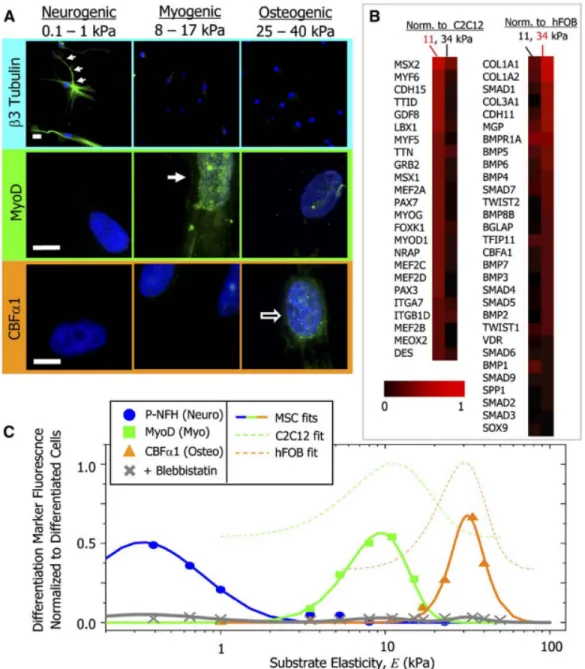
Figure 1.1.2 Protein and Transcript Profiles Are Elasticity Dependent under Identical Media Conditions..…..………..……..…………...…3
Figure 1.1.3 A model for direct force impact on gene activation………..………....…4
Figure 1.2.1 Main elements of a bio-AFM setup……….………7
Figure 1.2.2. Some AFM modes of operation……….………8
Figure 1.2.3 Overview of the theories generally used to interpret compressive force spectroscopic data...9
Figure 1.3.1: A cartoon depiction of the AFM with PRISM-LS………13
Figure 2.1.1 A system of conjugate planes..……….………….………18
Figure 2.1.2 Schematics of the system.……….………19
Figure 2.2.1. A light engine for two microscope systems………20
Figure 2.4.1 VIEW-MOD in an AFM sound hood.………23
Figure 2.4.2. Optical schematic for two light sheet pathways. ………..………24
Figure 2.4.3. Profile of LBS………..………25
Figure 2.5.1. Calibration of SM1 for LSFM.………...………26
Figure 2.6.1. ETL2 range for axial scanning.……….………27
Figure 2.7.1. Magnification and demagnification of ETL3.………..………28
Figure 2.7.2. Range of ETL3’s focus………..………28
Figure 2.8.1 Software design and hardware triggering for multicolor light sheet volume imaging...………30
Figure 2.8.2. Imaging setup for Horizontal Light Sheet.………..………31
Figure 2.8.3. Demonstration of a Horizontal Light Sheet stack with accompanying side view images.…..33
Figure 2.9.1. Initialization scan procedure for volumetric imaging.………34
Figure 2.9.2. Vertical light sheet volume imaging showed filopodia formation and dynamics.…….….……35
Figure 2.9.3. Fast Two-Color Volume Imaging of Live HeLa Cells.….………..………36
Figure 2.9.4. A 3D image sequence of phagocytosis with AFM.………37
Figure 3.2.1 Pictures of Optics………46
xi
Figure 3.3.2 Force plots of F-Tractin RAW cells.………..………53
Figure 3.3.3 Visualization of phagocytic cup evolution with AFM forces and light sheet side view imaging with RFP cells………..……….………58
Figure 3.3.4 Force plots of RFP cells.………
…
………59Figure 3.4.1. Vertical light sheet volume imaging showed filopodia formation and dynamics.……...……61
Figure 3.5.1 Light sheet volume imaging of macrophage phagocytosis.………..………62
Figure 3.6.1 Torque data from 3D phagocytosis experiment.………....……….…...…64
Figure 3.8.1 Forces in Dectin-1 mediated zymosan particle phagocytosis.……….68
Figure 4.2.1. 3D Nuclear Compression.……….……72
Figure 4.2.2. FRET Microscopy.………..…73
Figure 4.2.3. FRET Side View Imaging.……….…………73
Figure C.1 Numerical aperture of the y-z imaging plane.……….………..………….83
Figure C.2 Numerical aperture of the x-z imaging plane..……….…..84
Figure C.3Numerical aperture varies across height and position……….85
Figure C.4 Point spread function of side view imaging..………..……….86
Figure F.1.1 Thermal frequency spectra of cantilever……….……….94
Figure F.1.2Fourier Transform of fixed z-position time series…….…….……….94
xii
LIST OF ABBREVIATIONS AND SYMBOLS LBS Line Bessel Light Sheet
AFM Atomic Force Microscope InvOLS Inverse Lever Sensitivity
VIEW-MOD Versatile Illumination Engine With Modular Optical Design ETL Electrically Tunable Lens
AFM-LS Atomic Force Microscopy with Light Sheet Imaging PRISM Pathway Rotated Imaging for Sideways Microscopy
LS Light Sheet
LSFM Light Sheet Fluorescence Microscopy SPIM Selective-Plane Illumination Microscopy
LP1 Light Path 1
LP2 Light Path 2
SLD Super Luminescent Diode
IgG Immunoglobulin G
PBS Phosphate Buffer Solution FcɣR Fcɣ receptor
PI(4,5)P2 phosphatidylinositol-4,5-bisphosphate WASp Wiskott–Aldrich syndrome protein
µL microLiter
µg microgram
µm micrometer
nm nanometer
pN piconewton
1
Chapter 1: An Introduction to Current Needs in the Study of Cell Mechanics by Atomic Force Microscopy
Mechanical properties of internal and external cellular environments affect cellular behavior. This means that new techniques for probing the mechanical response of cells are needed to push the
boundaries of the field. Atomic Force Microscopy (AFM) is a technique that has been extensively used to study cell mechanics. Combined with light sheet microscopy and an innovative versatile optics system allows high frame rate and high-quality imaging, the AFM with a versatile optics system becomes a powerful tool to probe and observe cell behavior during mechanical stimulation. This chapter introduces the reader to the current state of cell mechanics, applications AFM in studying cell mechanics including AFM combined with fluorescent microscopy and the significance and goals of this project. The sections are:
1.1 Cell Mechanics
1.2 Use of Atomic Force Microscopy in Studying Cell Mechanics 1.3 Light Sheet Fluorescent Microscopy
1.4 Significance and Goals
1.1 Cell Mechanics.
Cells are the basic unit of biological life. They come in a myriad of shapes, sizes and functions. Understanding them is crucial to understanding of ourselves and of our health. Oftentimes, cells are described as a densely packed soup of biomolecules that respond to chemical and biochemical signals. While this is true, the past couple decades have revealed that cells also sense and respond to
2
mechanically. These range from the finger-like protrusions, filopodia,2,3 to the mechanically activated ion channels Piezo 1 and 2.4 For example, filopodia have a strong role in foreign pathogen identification and particle capture, a process known as phagocytosis, and in several diseases’ progression.5,6
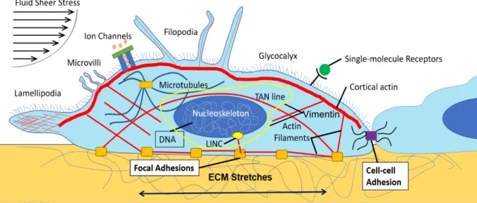
Figure 1.1.1. Cell Mechanical Sensing: Cells can respond to external mechanical stimuli, such as from the ECM, fluid flow, and other cells through cell-cell contacts. The ways they sense and respond to their mechanical environment is myriad. Some examples are drawn above. They include many from the cytoskeleton such as the many structures formed by actin, the LINC complex, focal adhesions, and microtubules. Single protein complexes, like Piezo ½ ion channels and receptors can respond to force. Even the nucleus, the vessel for the cell’s genetic information, is involved in mechanical sensing. We know that cell differentiate in large part due to mechanical cues from their environment (See Figure 1.1.2). In Engler, et al., stem cells grown on substrates of different stiffnesses expressed proteins corresponding to cell types in the body with similar environmental stiffness.7 This suggested that mechanical signals change gene expression in cells. Recently, direct evidence that this occurs through the stretching of chromatin has been published.8 A model for their particular application is shown in Figure 1.1.3.Besides basic biological research, the field of cell mechanics has informed our understanding of diseases. Failures in cellular mechanical interactions have been implicated in a host of disease states such as muscular dystrophies, emphysema, asthma, hypertension, and cancer.3 Cancer in particular is of interest to the field because cancer cells are, in general, softer than their wild type counterparts. And the softer the cells are the more invasive the cancer is 9. What determines a cell’s mechanical behavior is governed primarily by its cytoskeleton. The cell’s cytoskeleton is the interconnecting network of filaments and tubules that mediates forces involved in maintaining cell shape,
3
Figure 1.1.2 Protein and Transcript Profiles Are Elasticity Dependent under Identical Media
Conditions. (A) The neuronal cytoskeletal marker b3 tubulin is expressed in branches (arrows) of initially naive MSCs (>75%) and only on the soft, neurogenic matrices. The muscle transcription factor MyoD1 is upregulated and nuclear localized (arrow) only in MSCs on myogenic matrices. The osteoblast
4
Figure 1.1.3 A model for direct force impact on gene activation: A local surface force via integrins is propagated through the myosin II tensed actin cytoskeleton to the LINC (via SUN1 and SUN2) complex, to nuclear lamins, and is then transferred to the flanking chromatin through BAF and HP1 proteins and other molecules. The flanking chromatin transfers the force to deform and to stretch the chromatin segment containing the DHFR gene at the nuclear interior, facilitating binding of the RNA Polymerase II and transcription factors to upregulate DHFR transcription. Note that underneath each nuclear protein is its gene name. Not drawn to scale. This is figure 6 from Tajik, A. et al.8 Reprinted by permission from Springer Nature: Nature Materials. Transcription upregulation via force-induced direct stretching of chromatin. Tajik, A. et al. (2016).
5
Lam, et al., 2011;10
Adapted From: Liu, et al., 2012;11
Guck, et al., 2001;12 Galbraith et
al.,2002;13 Wang et
al., 200514,15
Adapted From: Håti, et al., 2015;16
Wang et al. 1993;17
Ziemann, et al., 1994;18 Adapted From: Poh et al.,
2009;19 Hu et al.,2004;
20
Spero, et al21
Ding, et al., 2013;22
Guo et al.,2015;23
Li et al., 201524
Adapted From: Topal et al., 2018;25
Yang and Saif, 2005;26 Polacheck
and Chen, 2016;27
Polacheck and Chen, 2016;27
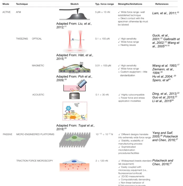
Table 1.1.1. Summary of common techniques for cell mechanical characterization. Table adapted from Basoli, Francesco, et al., 201828.
With the explosion of interest in cell mechanics research, new tools and techniques must be developed and old tools must be improved to further future research. Several common tools for studying cell mechanics with some advantages and limitations are listed in Table 1.1.1. Notice that each
application is designed to measure forces at specific parts of and directions toward the cell. The
6
ranges of forces to be measured. What is listed is typical force ranges used in the literature and should not be regarded as complete limitation. In the next section, AFM for cell mechanics studies will be introduced along with a more in-depth look at its function and versatility, as well as, attempts to integrate it with optical microscopy.
1.2 Use of Atomic Force Microscopy in Studying Cell Mechanics
Over recent years, Atomic Force Microscopy (AFM) has become an important tool for probing the mechanics of the cell.5 Although commonly used as a topographical imaging tool, in biophysical
applications, AFM is used to probe forces in tissue samples, cells, and even single molecules, detecting forces from the single molecule range of a few piconewtons to whole cell motions of several
nanonewtons. Because of its versatility and range of forces detectable, AFM is ideally suited for cell mechanics.
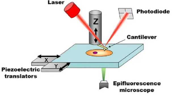
As illustrated in Figure 1.2.1, the basic operation of an AFM works by having a laser or super luminescent diode shine off the back of a cantilever onto a photodiode. A z-directed piezo lowers or raises the cantilever onto or near a specimen surface of interest. Once the cantilever draws near enough to interact with the surface forces, the cantilever will deflect either up or down. This deflection is detected by the photodiode via the laser and interpreted by Hooke’s Law as a force.
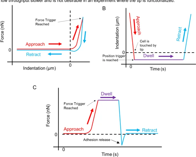
The AFM is capable of several modes of operation. For cell mechanics, AFM uses contact mode where the cantilever with a tip comes into contact with the cell. For performing measurements to find the stiffness of a cell, the tip is pressed into the cell until a force trigger point is reached. This portion is called the approach part of the force curve, as shown in Figure 1.2.2. Typically, a Hertz or Sneddon model is fit to the approach part of the curve to determine the stiffness of the cell. The user is able to choose whether to dwell for a time at that force level or immediately retract. In the retraction part of the curve, adhesion to the cell can be used in cell mechanics studies, such as the DMK model (see Figure 1.2.3). It also
provides useful information for cell surface molecule studies.
7
Figure 1.2.1 Main elements of a bio-AFM setup. The tip interacts with the probed sample and
attractive/repulsive forces cause the cantilever to bend. Bending is monitored by shining a laser light onto the backside of the cantilever and measuring the position of its reflected light using a four quadrant photodiode. A set of three piezoelectric positioners allow nanometer-scale movement of the tip with respect to the sample. The stage is typically moved in the x-y axis, while the cantilever is moved on the z axis. Other configurations are also commercially available, for example, x-y-z piezoelectrics moving only the cantilever or only the sample. In commercial systems, the AFM stage is fitted directly onto the body of the epifluorescence microscope (replacing its own stage), to allow seamless integration and an
unobstructed optical path for imaging. Adapted from Figure 1 from Gavara, N, et al.29
model such as the ones in Figure 1.2.3 to the force versus indentation data. In force trigger mode, or constant force mode, the AFM can also be used to set the force to dwell at a constant value for a
specified time. How the indentation evolves over time then becomes the important aspect to investigate. If a constant z-position mode is chosen, then how the force data evolves over time becomes the useful data. The two modes displayed in Fig. 1.2.2 (B) and (C) are used in the applications presented in this dissertation.
8
height above the substrate,31 but collecting height measurements for each cell would make an already low throughput slower and is not desirable in an experiment where the tip is functionalized.
Figure 1.2.2. Some AFM modes of operation: (A) Typical force curve with the approach part of the curve in red and the retract in blue. Once the AFM detects the force trigger has been reached after it is indented into the cell (starting at 0), it reverses direction, often faster than the cell relaxation can keep up with, as seen in the difference in approach and retract. (B) A constant position trigger uses the z-piezo to park the cantilever at a particular distance to the cell, typically right above or indented into the cell. Typically, the AFM dwells at this value for some time. In this mode, the force versus time plot is the relevant data because the end of the cantilever is free for the cell to move. (C) In constant force mode, the AFM will reach a force value and, with a dwell stay at that level until it retracts. Usually, there are detachment events of the tip from the cell surface. In this mode, the indentation versus time plot is the relevant data to analyze because it shows the cell’s positional change to the force applied.
In Schillers, H, et al.,a way of taking cell elasticity measurements was developed to enable more reliable
agreement between different AFMs called Standardized Nanomechanical Atomic Force Microscopy Procedure (SNAP).32 The procedure focused on improving sensitivity and spring constant calibrations. Rather than solely rely on manufacturer values or spring constants found through the instrument, they used a vibrometer to measure the spring constants. They found that the procedure increased the
Adhesion release
A
B
9
Figure 1.2.3. Overview of the theories generally used to interpret compressive force spectroscopic data: Various models used to obtain a measure of the Young’s modulus of cells, including the Hertz model (A); Sneddon model (C); and the Derjaguin–Muller–Toporov (DMT) model (D). (B) Depiction of the dynamic oscillatory model used to determine the visco-elasticity of cells. In each, the tip is colored grey and the indentation depth is δ; Adapted from Wang, Jiabin, et al., 2018.33
consistency of living cell elasticity measurements by a factor of two. I took the findings into consideration but ultimately decided to use the Sader Method for cantilever calibration.34 Moreover, the Sader Method has the advantage that the tip never needs to touch a surface before use, which is highly desirable for a functionalized tip.
10
with mechanical properties and toward imaging the plane directly beneath the AFM tip. For example, in
Yu, J Q, et al., they showed that AFM and Stimulated Emission Depletion (STED) imaging can
complement each other, differentiating topographical images and fluorescent signal.36 STED imaging with AFM combines nanoscale fluorescence imaging with the versatility of AFM, including AFM imaging, elastic moduli maps, adhesive mapping.36-40 These techniques illustrate the field’s desire for the ability to merge AFM single molecule force detection with single molecule imaging.
When performing AFM experiments in combination with plan view fluorescent microscopy, much of the information from the tip’s stresses on the cell is lost. Being able to see the side recovers the tip’s interaction with the cell. One common technique used to solve this problem is the confocal microscope. Confocal allows multicolor fluorescence imaging so different parts of the cell (and the AFM tip) can be imaged while the AFM probe presses into the cell. However, it suffers poor XZ resolution which is the important axis for correlating AFM tip-cell interactions with the imaging. This technique can acquire 3D images in a sub-second timescale, but with poor optical resolution. Most AFM with confocal systems will report 3D imaging on the order of 3-7 seconds to balance image quality and speed. Lim, et al., used spinning disk confocal imaging and determined that mechanically stimulating the cell with a functionalized fibronectin AFM bead tip caused RhoA activated cell stiffening.41 Several other similarly constructed AFM and confocal microscopes have found applications to cell mechanics.42-44
Harris, et al., is an excellent example of the benefits brought to investigations with the ability to
see side view with AFM.45 They used confocal slices to validate AFM tip indentation depth and found good agreement. However, a large discrepancy between elasticities found by using pyramidal tips and spherical tips showed that pyramidal tip’s area of contact with the cell was sometimes much greater than what the models assumed, leading to artefacts in the force data and erroneous fits. This suggested that part of the inconsistent elasticities reported in the literature could be due to these sorts of unseen interactions. For one aspect of their validation, the measurement of the Poisson ratio, the authors
11
determination of correct model parameters and will enable correlation of cell-tip interactions with force data to a greater accuracy.
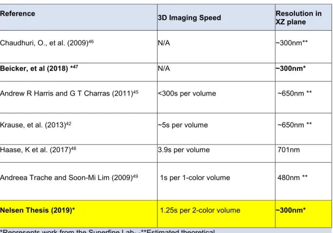
Side view fluorescence imaging with AFM has also been done on single cells with a separate side objective perpendicular to the illumination objective underneath the sample, but this setup restricts the ability for a user to choose appropriate cells as other techniques enable, including the one presented in this dissertation, and hampers the ability to perform 3D imaging.46 Table 1.2.1 summarizes several publications that demonstrate side view imaging and 3D imaging with AFM.
Previous work from our lab introduced Pathway Rotated Imaging for Sideways Microscopy (PRISM) for use with AFM.47 The system shows good XZ resolution with the use of while performing AFM measurements. Gaussian light sheet was added to the system which allowed greater contrast of
samples.47 This dissertation extends the PRISM with Light Sheet (PRISM-LS) capabilities to enable 3D scans of single cells in multiple channels and replaces the Gaussian light sheet with Line Bessel light
Reference 3D Imaging Speed Resolution in
XZ plane
Chaudhuri, O., et al. (2009)46 N/A ~300nm**
Beicker, et al (2018) *47 N/A ~300nm*
Andrew R Harris and G T Charras (2011)45 <300s per volume ~650nm **
Krause, et al. (2013)42 ~5s per volume ~650nm **
Haase, K et al. (2017)48 3.9s per volume 701nm
Andreea Trache and Soon-Mi Lim (2009)49 1s per 1-color volume 480nm **
Nelsen Thesis (2019)* 1.25s per 2-color volume ~300nm*
*Represents work from the Superfine Lab- -**Estimated theoretical
12
sheet (LBS). In the next section, I discuss the illumination technique of light sheet and why this type was chosen.
1.3 Light Sheet Fluorescent Microscopy
Light sheet fluorescence microscopy (LSFM), also referred to as selective-plane illumination microscopy (SPIM), has proliferated in recent years with applications to many areas of biology and at many scales of size, from single molecules50 to whole organisms.51,52 Inherent in LSFM’s advantages to other illumination techniques is its ability to acquire images at a high optical resolution and frame rate with low background fluorescence.
When scanned through a sample, LSFM allows for volume imaging of cells with low
photodamage.53-55 This allows capturing fast biological processes, most of which happen in 3D, with a high optical and temporal resolution with less bleaching of the sample. For these reasons, combining AFM with light sheet is ideal for moving toward single molecule imaging and correlating high frame rate imaging to forces. In order to use high resolution techniques with light sheet fluorescence microscopy on a conventional inverted microscope, several light sheet techniques utilize inverted SPIM (iSPIM)
13
Figure 1.3.1: A cartoon depiction of the AFM with PRISM-LS: A vertical light sheet from the objective illuminates the sample. A beaded tip cantilever sits above it. The light is collected. Adapted from Figure 2 in Beicker, K, et al.47
Additionally, we chose to use Line Bessel Sheet (LBS) for imaging. The system has the additional capability of using the Gaussian light sheet, but LBS has the advantage that it has a longer depth of field for the same beam width.66 Lattice light sheet67 (LLS) has a greater depth of field for the same beam width than LBS and is generally regarded as a superior illumination method to other light sheet
implementations. However, its implementation is significantly more cumbersome than LBS for our system. Moreover, as opposed to Bessel Beam illumination schemes,68 like LLS, or Airy Beam69 illuminations which take a beam and oscillate it to create the 2D plane, the LBS requires no rapid oscillation, reducing vibrations that the AFM could detect. For these reasons, LBS was chosen for the majority of the
experiments performed here.
14
use fast scanning piezos on the stage to move the sample.66 To avoid vibrations in the force data, we chose a remote focusing technique using an electrically tunable lens on the output side to change the focal plane while scanning the light sheet. Our single cell 3D scans are on the order of a second, comparable with similar techniques.66,67 For a more extensive treatment of the light sheet proliferation, I refer the reader to Girkin, J M, et al.,54 for an extensive list of light sheet techniques and their descriptions. In the next section, I explain the significance and goals of each chapter in this document.
1.4 Significance and Goals
There are two parts to the significance of this research: The general significance of the instrumentation development of the AFM with a versatile optics system and the significance of its application to phagocytosis.
First, for the AFM with a versatile optics system, my goal has been to develop an instrument capable of performing sensitive force measurements with the ability to correlate them to high resolution images. To that end, in chapter 2, I discuss the versatile optics system, referred to as Versatile Illumination Engine With a Modular Optical Design (VIEW-MOD) and its advantages for flexible switching between
microscopy techniques. I focus on the VIEW-MOD microscopy applications for AFM, namely, two-color fixed Line Bessel light sheet imaging and whole cell volume Line Bessel light sheet imaging. This system allows controlled forces to be applied to individual living cells and tissue with synchronized imaging and a myriad of switchable microscopy techniques. This combines many advanced microscopy techniques into one set up with the design and open source software disseminated to the scientific community. Much of the work in this project has been devoted to the design and implementation of this system. Being able to see controlled forces from different views (plan view and side view) with different microscopy techniques opens exciting, unexplored avenues of biophysics research.
15
phagocytosis works. Understanding phagocytosis will lead to a better understanding of how to fight disease.
This document is organized in the following way:
1. In Chapter 1, I have provided an introduction to cell mechanics, AFM applied to cell mechanics studies and light sheet microscopy. I highlighted a few of the needs for the field and how the current instrument meets those needs or improves current approaches. 2. In Chapter 2, the design and characterization of VIEW-MOD as it fits into applications for
AFM cell mechanics studies is described. This system is the first to do two-color light sheet imaging with synchronized AFM data, the first to do LBS light sheet imaging with
synchronized AFM data, the first to do whole cell light sheet volume imaging with synchronized AFM data, and the first to do two-color light sheet volume imaging with synchronized AFM data. This system has XZ resolution comparable to theoretical resolution of other systems, but with more capabilities and flexibility. The AFM allows piconewton level force measurements.
3. In Chapter 4, I applied the AFM with Line Bessel Sheet to the mechanics of phagocytosis. Here I demonstrate the first system to do AFM with macrophage FcɣR mediated and Dectin-1 mediated phagocytosis and the first to do volume imaging of phagocytosis with synchronized AFM data.
16
Chapter 2: A Versatile Optics System for use with Atomic Force Microscopy Cell Mechanics Studies
Fluorescence microscopy (FM) is one of most powerful techniques in biological and biomedical research. A handful of FM techniques have been developed to accelerate acquisition speed, improve resolution, reduce
background and reduce photodamage, either to the cell or the fluorophore. The excitation strategies of FM can be divided into three major categories: widefield, point-scanning, and light-sheet illumination. In a widefield configuration collimated light exits the objective illuminating the entire sample. With point-scanning, the objective focuses a collimated light source onto a diffraction limited point, which is raster scanned across the sample to render an image. In LSFM, a thin sheet of excitation light is created either by focusing one axis of the illumination source or rapidly scanning a focused beam along a single direction. Scanning the light sheet across the sample can then create a 3D volume. In this chapter, I introduce this versatile optics system, referred to henceforth as VIEW-MOD. I will emphasize the implementation of the modalities which add to our LSFM capabilities, but I will make mention of some other notable techniques as their modalities are encountered. While not exhaustive, a more extensive list of the capabilities in this system can be found in Appendix A. As a general outline to this chapter, first, I will discuss the original purpose of the system’s development. Then I move through the optics pathway and the purpose and characterization for each modality, starting with the light engine and moving to image capture. Finally, I will discuss the additions to the system made specifically for achieving live cell LSFM imaging with AFM.
Much of this work is taken from a paper, titled “VIEW-MOD: A Versatile Illumination Engine With a Modular Optical Design for Fluorescence Microscopy,” authored by Bei Liu, Chad Hobson, Frederico M. Pimenta, Evan Nelsen, Joe Hsiao, Timothy O’Brien, Michael R. Falvo, Klaus M. Hahn, and Richard Superfine. The paper is published in Optics Express volume 27, issue 14, and found in pages 19950-19972. Any figures taken from the paper will be labelled as Liu, Bei, et al.15,76
The sections in this chapter are as follows:
17 2.3 Modality 1: Beam Expansion and Polarization.
2.4 Modality 2: Switchable Pathways for Light Sheet and Point to Wide-field Illumination. 2.5 Modality 3: Fast Steering Mirrors for Beam Steering.
2.6 Modality 4: A 4f Configuration for Axial Beam Scanning. 2.7 Modality 5: A 4f Configuration for Axial Image Scanning. 2.8 Implementing Live-cell Light Sheet Fluorescence Microscopy. 2.9 Whole Cell Fast Volume Imaging for Use with AFM.
2.10 Conclusion.
2.1 Introduction to VIEW-MOD: The Versatile Optics System Design and Motivation
VIEW-MOD was designed for the specific purpose of enabling AFM to combine with 3D imaging. However, as the design was implemented, our lab found that with minimal modification, several other microscopy techniques could be included. This optical engineering was accomplished through the use of conjugate planes. As shown in Figure 2.1.1, the system was designed to have several planes in the illumination pathway at equivalent positions to manipulate the beam, either diverging or collimated, far from the objective lens. The line BFP, is conjugate to the back focal plane. The line SP is conjugate to the specimen plane. As one might guess, mirrors for directing the beam are located at those planes. At the red line, a tilt there corresponds to a tilt at the back focal plane of the objective. As the beam exits the objective lens, the specimen will then see a lateral translation of the beam in x and y axes parallel to the sample stage. At the blue line, a tilt corresponds to a tilt at the specimen plane. The specimen will see the beam tilt at an angle with respect to the z axis, the axis perpendicular to the stage.
In Figure 2.1.2, an optical schematic showing the general pathway with each modality labeled with a number. I will refer to each of the modalities by their number label in explaining how a certain imaging technique is accomplished. The light engine is not included in the schematic because it is assumed that all the imaging modes will be using lasers originating from the light engine.
18
Figure 2.1.1 A system of conjugate planes. The system is designed to have control of the front and back focal planes of the 60x 1.2NA Water objective lens far from the specimen plane. This allows
versatility of the imaging techniques employed and easy access to the optics. The series of relay lens act to propagate the beam along the path. In the case of LSFM, each axis alternates between collimated and converging as it passes through the system, as shown in the top and bottom of the figure. RL=Relay Lens; ETL=Electrically Tunable Lens; TL=Tube Lens; BFP=Back Focal Plane; SP=Specimen Plane. above, in module 3, fast steering mirrors tilt the beam causing the respective conjugate plane of the objective lens to tilt. In module 4, a 4f lens configuration decouples the illumination beam from the objective lens height, enabling axial beam scanning, that is, along the z axis of the specimen plane. In module 5, the only detection pathway module, a 4f lens configuration decouples the imaging plane from the height of the objective. Relevant portions of each module are controlled with computer software by the user. This allows flexibility for the use of each module and rapid switching from one imaging technique to another.
Conjugate planes Conjugate
planes
19
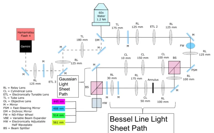
Figure 2.1.2 Schematics of the system. Linearly polarized lasers are expanded, collimated and exit Module 1. The light propagates to Module 2 through either pathway 1 (blue dashed-line) for TIRF and point-scanning or pathway 2 (red dashed-line) for LSFM, depending on the orientation of its polarization axis. For TIRF, ETL1 is adjusted to 125 mm effective focal length to focus the beam onto SM1, resulting in a collimated light beam coming out the objective. For point-scanning ETL1 is set to ~ 0 volts, equivalent to f=∞ (flat plate). Steering Mirrors 1 and 2 (SM1 and SM2) are optically conjugated with the specimen plane and the Back Focal Plane (BFP) of the objective, respectively. For LSFM, we either put a 125 mm cylindrical lens to create a Gaussian light sheet or use a combination of cylindrical lens and annulus to create a Line Bessel Sheet (LBS). ETL2 provides axial scanning of the illumination light. In the detection module (Module 5), the image is projected to the camera through a relay lens group (RL1 and RL2) with ETL3 placed in the center (mimicking Module 4) to achieve an adjustable image plane. Schematic was generated with GW Optics component library (http://www.gwoptics.org/ComponentLibrary/). Image Credit: Bei Liu, from Liu, Bei, et al.76
2.2 Light Engine Design and Characterization.
A versatile optics system would not function without a laser source to power it. The light engine described herein was designed to allow automatic computer control of multiple laser wavelengths.
20
Furthermore, the laser beams are split with independent control, allowing separate microscopes different laser needs to operate at the same time.
Figure 2.2.1. A light engine for two microscope systems. Four laser lines, 445nm, 488nm, 514nm, and 561nm are aligned along the same path by adjusting each laser set of two tilt mirrors. Each laser beam is reflected off a long pass mirror which allows longer wavelengths through but not its own. It is now colinear with the others. The beam is split evenly into two paths. The AOTF filters the wavelengths and their respective power levels before the laser is coupled into the fiberoptic cable. Image Credit: Chad Hobson
21
incoming light into two primary beams: One that goes to a light stop and one that couples into the fiberport. Changing the power supplied to the crystal changes the amount of light diffracted to one beam or the other. Furthermore, the acoustic wave frequency can be adjusted, enabling the user to select which laser, or lasers if more than one frequency is chosen, can pass through.
Finally, the fiberports and fiberoptic cables must be discussed. Of foremost importance is choosing a fiberport that is compatible with the fiberoptic cable. Fiberoptic cables have a limited range of wavelengths that they can accept without having drastic differences in the laser power for wavelengths out of range. The fiberport must be rated for the wavelengths that are used, it must be matched to the fiber type, allowing either single mode or multimode and whether it is polarization maintaining, and it must have the desired lens type, either achromatic or aspheric. Furthermore, paying attention to the numerical aperture of the fiberport lens helps to optimize power output and to make alignment more manageable with the fiberoptic cable. Alignment of the fiberport is sensitive, even to temperature changes, so taking care to match it with the fiberoptic cable is worth the effort. For the fiber optic cable, one was selected that was rated for the wavelengths shown in Figure 2.2.1. Much of the light is lost in coupling to the fiberoptic. For the fiberoptic cable used by this system, a good coupling will see only 25% of the light exiting out the other end. This ends up being more than enough for the experimental purposes. Also, back reflections were a problem in a previous fiber, which was remedied by switching the fiber for one with an anti-reflective (AR) coating.
In the next five sections, I will discuss VIEW-MOD, starting with the sizing of the beam after the laser light exits the fiberport.
2.3 Modality 1: Beam Expansion and Polarization
22
optimizing the depth of field of a Gaussian light sheet for a larger specimen than a single cell. The polarization axis of the light exiting the optical fiber is then adjusted by either rotating a half-wave plate (AHWP05M-600, Thorlabs) or through a liquid crystal retarder (LCC1111T-A, Thorlabs). A polarized beam splitter redirects the light either to light path 1 (LP1) or light path 2 (LP2) of module 2 to switch between a circular beam cross section or a cylindrical (light sheet) cross section. The polarized beam splitter determines the orientation of the polarization of the beam, and the tunable waveplate governs the amplitude of the light going into each arm of module 2. Because each wavelength of laser light exits the fiber at a different polarization, the tunable waveplate becomes important to switch to the
optimum setting for each wavelength. It is critical if as much light as possible is needed for an application. Notice that the system is designed such that when using light sheet illumination, the polarization vector of the laser beam is normal with respect to the plane of the light sheet. In some cases, it may be useful to switch the polarization state of the illumination beam at the specimen. That can be accomplished by adding a second waveplate after module 2. The use of a tunable waveplate allows computer control of these operations.
2.4 Modality 2: Switchable Pathways for Light Sheet and Point to Wide-field Illumination.
23
geometries in a single system allows one to employ drastically different illumination techniques (e.g., LSFM and point scanning) on a single sample.
Point illumination is a powerful technique as it allows researchers to selectively illuminate a portion of the
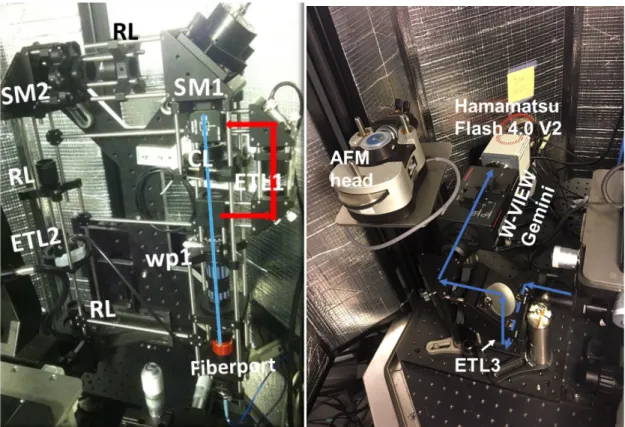
Figure 2.4.1 VIEW-MOD in an AFM sound hood. A labeled image of VIEW-MOD modules 1-4 (left) fitting inside an AFM sound hood. Following through module 1 and the waveplate (wp1), the beam path can either go through the cylindrical cross-section (blue) or the circular cross-section (red) light path. Module 5 (right) is shown. It too fits comfortably in the sound hood, showing the AFM head, ETL3, Gemini optics splitter and Hamamatsu Flash 4.0 V2 sCMOS camera.
sample without perturbing other areas. This technique is particularly useful in the field of optogenetics to precisely activate or inhibit particular proteins with precise spatiotemporal resolution. However most of the most microscope systems were carried out with either a separate photoactivation module77 or a commercialized confocal
24
full field of view. Optotune released a 20 dipoter ranged ETL, which is sufficient to cover the field of view and is used in the two other VIEW-MOD set ups.
Figure 2.4.1 also demonstrates the engineering challenge in building VIEW-MOD. It needed to fit in an AFM sound hood and still fit on the vibration isolation table. The tight spatial constraints forced my lab to build VIEW-MOD vertically with respect to the vibration isolation table. The two other VIEW-VIEW-MOD microscopes are not subject to such constraints so are laid out on a horizontal optical table.
The Superfine lab decided to switch the point illumination light path to another light sheet mode, LBS. The
Figure 2.4.2. Optical schematic for two light sheet pathways. The schematic for LBS and Gaussian light sheets is shown above. Adding LBS to the system demonstrates VIEW-MOD’s flexibility to replace old or infrequently used pathways with new or improved techniques to the system while still maintaining ones currently in use. Image credit: Chad Hobson.
25
optically conjugate to the BFP of the objective. When the two coherent bands pass through the objective lens (UplanSAPO 60x/1.2 W, Olympus), they interfere with each other resulting in a Line Bessel Sheet66.
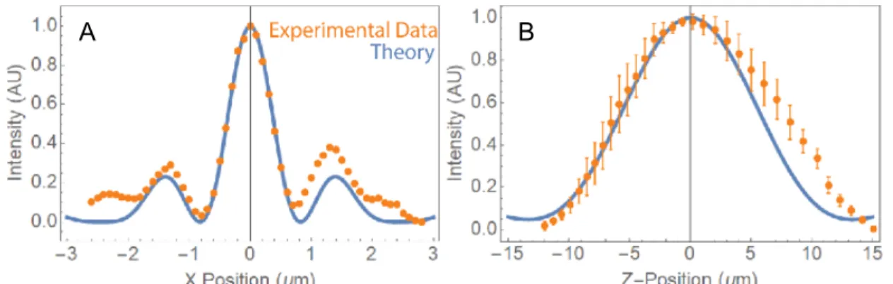
The profile of LBS is shown in and the z axis profile is shown in Figure 2.4.3. The measured lateral and axial FWHM of the LBS is 771 nm (Figure 2.4.3(a)) and 14.8μm (Figure 2.4.3(b)) respectively, both of which match
Figure 2.4.3. Profile of LBS. (A) Lateral profile of the LBS. A 100 nm fluorescent bead was stepped laterally in 100 nm increments by a piezo stage; intensity of the bead was measured in FIJI for each position. (B) Axial profile of LBS. 100 nm fluorescent beads were imaged as the LBS was stepped axially by ETL2 in 2 mA increments. Intensity of 7 beads was tracked across the scan in FIJI, error bars are standard deviations in intensity. Orange represents measured intensity from the fluorescent beads; blue represents a theoretical profile. Calculations and measurements were performed by Chad Hobson. well with the theoretical value79,80. A Gaussian light sheet at 561nm wavelength with a comparable waist size (0.65µm) will have a FWHM of the depth of field of about 5 µm. The current Gaussian waist size is 1µm, which provides a 11µm FWHM depth of field. Cells are often taller than 11µm, so LBS enables clear imaging of the whole cell while maintaining better sectioning capability. This is the primary reason why the majority of the data presented in this dissertation was completed with LBS. Additionally, for reasons unique to this set up, LBS is easier to align than the Gaussian light sheet.
2.5 Modality 3: Fast Steering Mirrors for Beam Steering.
As mentioned previously, Module 3 controls the steering of the illumination light both at the BFP of the objective and at the sample plane using two fast steering mirrors (SM1,2) (OIM 101 1”, Optics In Motion LLC). SM1 is optically conjugate to the BFP of the objective while SM2 is optically conjugate to the sample plane. The former controls the position of the beam at the sample plane and the latter adjusts the tilt at the sample plane. SM1 and SM2 are driven by voice coils and are each able to control two axes of tilt in a single mirror. This allows a more compact design for optical conjugation with a single mirror compared with using galvo-scanners, which typically needs two mirrors in a 4f configuration. While galvo-scanners are notably faster, SM1 and SM2 can execute a 1
26
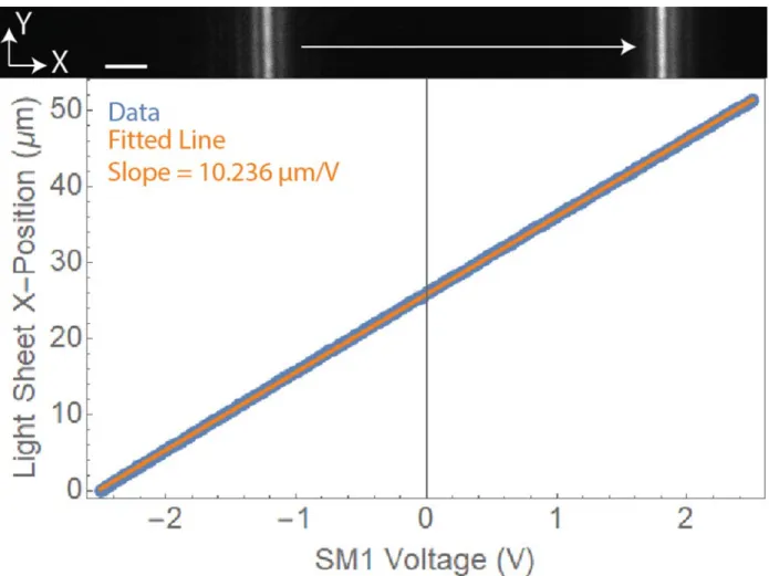
mrad step in under 5 ms, providing enough speed for sub-second volumetric imaging. In Figure 2.5.1, a calibration for lateral light sheet scanning is shown. To calibrate SM1, we used an autofluorescent slide (92001, Chroma) on the microscope specimen stage. SM1 voltages were scanned from in increments of 1 V with an image acquired at each voltage ordered pair by the imaging sCMOS camera (ORCA-Flash4.0 V3, Hamamatsu).
SM1 and SM2 are controlled by four channels of analog voltage supplied by a National Instrument (NI) DAQ board (PCIe-6323). For light sheet volume scanning, SM1 needs to be calibrated to establish the
correspondence between the control voltages and the beam position the sample plane. A lab-built MATLAB
Figure 2.5.1. Calibration of SM1 for LSFM. Calibration of SM1 showing the light sheet x-position versus voltage applied to SM1 as well as a linear fit to this data. The slope of the linear fit provides us a conversion from SM1 voltage to scanning distance, allowing us to understand and properly set our voxel size during volume imaging. Scale bar = 5 µm.
27
variable angle total internal reflection fluorescence microscopy (vaTIRF). In that application, SM2 is used to tilt the beam to maintain the critical angle needed for vaTIRF.
2.6 Modality 4: A 4f Configuration for Axial Beam Scanning.
Module 4 provides control of the axial, along the z-axis, position of the illumination light without physical displacement of the objective lens. Keeping the objective motionless is ideal as it reduced small motions of the sample that are coupled to objective movement. A 4f system with a second ETL (ETL2) (EL-16-40-TC, Optotune) midway between the second and third relay lens (conjugate to the BFP of the objective) relays the beam. Adjusting the focal length of ETL2 subsequently scans the focus of the illumination light axially81. This is useful for both LSFM and point scanning to ensure that the tightest focus of the illumination light is at the desired location in the sample. As shown in Figure 2.6.1, ETL2 has a range of greater than 120µm. The large range is critical for PRISM-LS where
28
the objective must focus high on the microprism for image formation. As the objective raises up, the light sheet is raised with it. Subsequently, the light sheet must be lowered to ensure the thinnest portion is used, and thus the best image is formed.
2.7 Modality 5: A 4f Configuration for Axial Image Scanning.
Module 5 is an identical 4f system to that of module 4, except it lies in the detection path. Similar to Module 4, we place an ETL (ETL3) (EL-16-40-TC, Optotune) midway between two relay lenses. Adjusting the focal length of ETL3 then shifts the axial position of the imaging plane74,82,83. One can dynamically manipulate the focus of an image during an experiment without moving the objective lens or the illumination light. Without this capability, the objective must be stepped incrementally for an image stack and its movements would be detected by the AFM. It should be noted that large scale changes of the optical power of ETL3 will (de)magnify the image84,85 . Other groups have used an ETL for axial control of the imaging plane by placing the ETL directly behind the detection
Figure 2.7.1. Magnification and
demagnification of ETL3. This plot shows ETL3’s magnification percent change relative to the resting voltage (4.76V) image in the
detection path. ETL3 ranges from -10V to 10V. Only 0-10V is shown here because it is well beyond normal operation. Normal operation is <1% magnification, designated as between the red, dashed lines.
Figure 2.7.2. Range of ETL3’s focus. ETL3 is capable of 60µm of imaging above or below the focal plane of the objective. This allows for rapid switching between plan view and side view, which is helpful for side view in determining where the tightest focus of the light sheet resides. Typical side view operation has plan view approximately left of the orange dashed line, assuming side view is visible at 4.76V (zero focal plane position). A Typical range for side view volume imaging is shown
between the horizontal red dashed lines. The range is usually around half a volt, which as can be seen will traverse ~15µm. Figure adapted from Liu, Bei,
et al.76
6 4 2 0 2
0 2 4 6 8 10
Magnificationrelativeto restingvoltage 4.76V image
29
objective84-89, however using ETL3 in a 4f system makes it easier to access and adjust as well as minimizes the (de)magnification effects74,83. Even at the limits of ETL3 operation in this module, the magnification is at most 6%, as shown in Figure 2.7.1. Normal operation of ETL3 is within 1% of the resting state voltage magnification. Moreover, ETL3 lies flat (its optical axis is normal to the table) to avoid gravitational effects which would distort the Optotune lens. A controller (Gardasoft Inc.) for ETL3 is programmed to the linear analog mode (0 V – 10 V) and outputs a current based on a closed-loop temperature feedback system. To calibrate ETL3, we place a grid (R1L3S3, Thorlabs) on the microscope and manually step the objective lens position. ETL3 is used to bring the grid back into focus, providing a calibration of ETL3 voltage with the imaging plane position. Figure 2.7.2 shows the range of ETL3’s axial focal plane manipulation. Imaging plane location, light sheet position and AOTF are synchronized through an NI DAQ board.
2.8 Implementing Live-cell Light Sheet Fluorescence Microscopy.
To implement LSFM, we employ modules 1-5. Module 1 properly sizes the beam and rotates the polarization state such that the light passes through LP2, the cylindrical cross section path of module 2, and the polarization vector is normal with respect to the plane of the light sheet.
Modules 3 and 4 provide complete control of all three spatial positions of the illumination light while module 5 allows us to adjust the axial position of the imaging plane. We use a lab-built LabView program that controls two NI DAQ boards (PCIe-6323 and PCI-6723); one controls voltages to the SM1 controller and ETL3 controller (TR-CL180, Gardasoft) while the other controls the AOTF in our light engine to gate the laser light. A diagram of the triggering scheme is shown in Figure 2.8.1. Because synchronizing AFM and imaging data is critical for correlation, the NI DAQ boards are triggered by the AFM output signal. This allows the start of the imaging to coincide with the start of the AFM cantilever lowering onto the substrate. Our lab uses the Optotune software to control the current applied to ETL2 which subsequently varies the optical power.
As noted earlier, SM1 is conjugate to the BFP of the objective. Tilting SM1 translates the LBS in x-y at the sample plane. For volumetric imaging, we need to control only the translation of the LBS in the x direction
30
Figure 2.8.1 Software design and hardware triggering for multicolor light sheet volume imaging. The AFM ARC controller, which is operated by software developed by Asylum Research, sends an analog voltage signal to the two NI DAQ boards. This synchronizes the force data being collected with the imaging components. One board then sends a voltage signal to trigger the camera and choose the desired laser wavelength(s) and power(s). A second board sends a voltage signal to the mirror and ETL3. In volume imaging, the steering mirror and ETL3 are triggered based on a lookup table generated through a MATLAB program. The synchronization software is run off of LAB-View (National Instruments).
Separate to this synchronization scheme is the lab-built software used to control the scanning mirror, ETLs, Camera and AOTF with a computer GUI. This software is a combination of Hamamatsu HCImage Live, LAB-View and MATLAB programs. Software was developed primarily by Joe Hsiao.
calculating the voxel size.
31
Figure 2.8.2 Imaging setup for Horizontal Light Sheet. (A) The light sheet emerges from the objective and is reflected by a right-angle prism. The focal plane is matched to the plane of the reflected light sheet. (B) Imaging setup for Vertical Light Sheet. The light sheet emerges from the objective and creates a vertical slice through sample. The right-angle prism creates a virtual side-view image of the vertical slice. (C) Horizontal light sheet image of a RAW 264.7 cell labelled with Cholera-toxin b AlexaFluor488. (D) Vertical light sheet images of HeLa cell stained with Phalloidin-AlexaFlour594. The HeLa cells are a gift from the Lab of Dr. Michael Boyce. Figure is adapted from the VIEW-MOD manuscript (A, B drawn and C collected by Chad Hobson).
32
high resolution images of the plane in which the AFM tip is applying force without the need for taking whole stacks42,90,91 .
Streaking in this image due to shadowing effects, which are common in light sheet microscopy.92 These streaks are the result of debris on the prism, which demonstrates the importance of using clean prisms. They are more pronounced here because of where the light sheet is hitting, that is, near the bottom of the prism where biological debris frequently accumulates. More on the protocol for cleaning prisms can be found in Appendix D. The disadvantage to using horizontal light sheet is the inability to view cell-AFM tip interaction with the same certainty as in side view. This can be overcome if volume scans of the horizontal light sheet is implemented. A side view image of a fixed HeLa cell stained with Phalloidin-AlexaFlour594 is shown in Figure 2.8.2 D. This is PRISM-LS representative imaging of cytoskeleton proteins, such as the actin shown. This is important for studying cell mechanics with AFM that load bearing proteins, such as actin, are visualized.
Volume imaging is capable of being accomplished using HLS, but was not implemented. To demonstrate that volume imaging can indeed be implemented using HLS, I took images of five sections of a macrophage. As shown in Figure 2.8.3, using side view I can determine where on the cell the light sheet is illuminating. This demonstrates that HLS with PRISM is capable of illuminating the whole cell, from top to bottom, which is not available in all HLS configurations.50 We image the cells in plan view, a form of single objective Single Plane Illumination Microscopy (soSPIM). This form of illumination is common for biological imaging but suffers from the lack of flexibility to choose the cells most appropriate for the experiment.63-65,82 Our translation and tilt stage for the microprism solves this problem by allowing us to choose which cell is best for imaging and AFM probing (TTR001, Thorlabs).
33
maintained at 37oC with 1.5oC drop at the edge of the coverslip. More information about temperature control can be found in Appendix E. In the next section, I discuss fast whole-cell volume imaging for AFM.
Figure 2.8.3. Demonstration of a Horizontal Light Sheet stack with accompanying side view images. (A) Brightfield image of the RAW cell in plan view. (B) Side view of the cell with Gaussian light sheet. Cell is labelled with Cholera toxin b-AlexaFluor488. (C) Side view of the cell with horizontal light sheet at different heights showing a line of fluorescence where the light sheet is located. (D) The plan view image of the horizontal light sheet at different planes. The planes lower from top of the cell to the bottom of the cell. The side views are approximate locations of HLS. (E) Shows a cartoon of the
horizontal light sheet location and side view imaging for (C). The focal plane is labelled as a black dashed line. (f) Shows a cartoon of the horizontal light sheet location and plan view imaging for (D). The focal plane is labelled as a black dashed line.
E
Focal Plane PRISMF
PRISM34 2.9 Whole Cell Fast Volume Imaging for Use with AFM.
This microscope design with LBS illumination is also capable of fast volumetric imaging by incrementally stepping the light sheet across a sample and continuously matching the imaging plane to the position of the light sheet.SM1 stepped the LBS in increments laterally in the x-axis through the cell. ETL3 was adjusted such that at each step the image was in focus. Every time the mirror was brought down next to a cell of interest, the spacing of the cell and mirror was different and the angle of the mirror relative to the substrate was slightly varied due to the mechanical micrometer control mechanism. For each cell we performed an initialization scan (Figure 2.9.1) yielding a lookup table of the ETL3 voltage value that provided the best focus for each LBS position in the volume scan. With
Figure 2.9.1. Initialization scan procedure for volumetric imaging. (A) A sample mini scan of a COS-7 nucleus expressing HaloTag-H2B labeled with Janelia Fluor 549 used in the initialization scan where the LBS is fixed to a specific location and the ETL3 voltage is varied about a suggested voltage of best focus. The Tenegrad method93,94 is used on each image from the mini scan to provide a metric for image quality. A Gaussian is fit to the mini-scan data to provide the optimal ETL3 voltage for a given light sheet position. (B) A sample lookup table that provides the best ETL3 voltage for a given light sheet position. Each orange data point is generated by a mini scan procedure. A linear interpolation is done between data points and is discretized based upon the number of slices per volume. Figure is from Liu, Bei, et al.15
this lookup table we performed fast volume scans of RAW 264.7 macrophage cells stably expressing HaloTag-F-Tractin labeled with JF549 (Figure 2.9.2). Each slice was taken in 10 ms (5 ms exposure, 5 ms transition), and each volume consisted of 75 slices meaning that a single volume image was taken in 0.75 s; this is comparable to recent two-objective systems66,67,84. Because of the speed of our system, we were able to observe both formation and movement of filopodia on the timescale of several seconds. These timescale dynamics are fundamental to
35
Figure 2.9.2 Vertical light sheet volume imaging showed filopodia formation and dynamics. Selected frame from a volumetric movie (Visualization S4) of a RAW 264.7 macrophage cell expressing HaloTag-F-tractin labeled with JF549. Each volume consists of 75 slices each taken in 10 ms (5 ms exposure, 5 ms transition time) for a 0.75 s total volume acquisition time with 100 ms delay between each volume. Total volume size is 12.5 µm x 26.7 µm x 25.9 µm, voxel size is 167 nm x 106 nm x 106 nm. We observed formation and movement of individual filopodium on second time scales. Image Credit: Chad Hobson. Figure taken from Liu, Bei, et al.76
We further demonstrated the potential of our microscopy method’s 3D scanning capability, 3D PRISM-LS, by taking 3D two-color scans of HeLa cells with Lysotracker-Red (Figure 2.9.2 A) and Vimentin-mEmerald (Figure 2.9.3 B). Each two-color whole-cell scan was taken in 1.5s, with 10ms for each slice. As a result of the volume imaging, we can track a lysosome in 3D through several slices of the specimen, as highlighted in Figure 2.9.3 C.
36
stably expresses HaloTag- FTractin labeled with JF594. In Figure 2.9.4, I took a series of 3D images while 2.85s per two-color volume, which corresponds to a 10 ms camera exposure time and 5 ms camera readout time. I included a 7s delay between each volume scan to reduce photodamage over the 30-minute experiment. The bead is not shown, but its location can be surmised by the location of the phagocytic cup. Part of a second cell is seen in the background and is far enough away from the cantilever not to affect the experiment. More on this data set will be explored in Chapter 3.
Figure 2.9.3 Fast Two-Color Volume Imaging of Live HeLa Cells. Live HeLa cells stably expressing vimentin-mEmerald, an intermediate filament, shown in (A) and dyed with LysoTracker Red, shown in (B), are 3D imaged at a rate of 1.5s per volume. At 75 frames per color, this corresponds to a camera readout of 5ms and exposure of 5ms. 100ms delay is added in between volumes. Voxel size is 106 nm x 106 nm x 220 nm. Lysosomes are able to be tracked across image planes over a short time span. The cells are a gift from the lab of Dr. Michael Boyce. Volumes imaged by Chad Hobson.
A
B
C
t : 0 s
t : 64 s
37
Figure 2.9.4 A 3D image sequence of phagocytosis with AFM. A RAW 264.7 cell is shown attempting to engulf the AFM bead tip (not shown) functionalized with IgG. 2.85s per two-color volume, which corresponds to a 10 ms camera exposure time and 5 ms camera readout time. A 7s delay is included between each volume scan to reduce photodamage over the 30 minute experiment. The voxel size is 106nm x 106nm x 200nm, with the 200nm dimension in the light sheet stepping direction. 78.8, 453.1, 1280.5, T1940.45s is after the AFM retracted. The large adhesive force at retraction shows the cell is well attached to the bead.
2.10 Conclusion.
38
Chapter 3: Force spectroscopy of phagocytosis with Bessel light sheet imaging
A critical part to the immune system is the search and elimination of foreign pathogens by macrophages, neutrophils and other cells. These cells eliminate large particles (>0.5μm) by consuming
them through a process called phagocytosis. There are several receptor and ligands pairs with their associated signaling pathways that initiate phagocytosis. The best understood is the Fcɣ receptor (FcɣR)-immunoglobulin G (IgG) pair. Recognition by FcɣR of an IgG coated particle triggers the cell’s
cytoskeleton to form a pseudopod that reaches around and engulfs the particle. Understanding the mechanics of how a macrophage engulfs a target requires careful monitoring of forces and high-quality fluorescence imaging of the membrane and cytoskeleton. The goal of this chapter is to determine the evidence for force dependent phagocytosis models. In a first of its kind, we combined an atomic force microscope (AFM) with a versatile optics system to monitor piconewton scale forces while imaging the phagocytosis engulfment from the side using VIEW-MOD with vertical light sheet. The macrophage produces a dynamic response of a few nanonewtons during its envelopment of an IgG covered AFM tip. The macrophage exerts downward forces on the bead before the pseudopod envelops past the midpoint of the bead. The cup formation is associated with punctate brightening of actin underneath the bead. A less well understood process is Dectin-1 mediated phagocytosis. Dectin-1 recognizes ꞵ1 and ꞵ3-glucans which are present on pathogens such as fungi. In a first, Bessel beam light sheet imaging with controlled force data will inform mechanical models of phagocytosis which will improve understanding of this important immunological process and inform mammalian disease progression.
This chapter aims to discuss measuring forces in phagocytosis. The sections in this chapter are as follows: